- MapReduce Algorithm
- Linear Programming using Pyomo
- Networking and Professional Development for Machine Learning Careers in the USA
- Predicting Employee Churn in Python
- Airflow Operators

Solving Transportation Problem using Linear Programming in Python
Learn how to use Python PuLP to solve transportation problems using Linear Programming.
In this tutorial, we will broaden the horizon of linear programming problems. We will discuss the Transportation problem. It offers various applications involving the optimal transportation of goods. The transportation model is basically a minimization model.
The transportation problem is a type of Linear Programming problem. In this type of problem, the main objective is to transport goods from source warehouses to various destination locations at minimum cost. In order to solve such problems, we should have demand quantities, supply quantities, and the cost of shipping from source and destination. There are m sources or origin and n destinations, each represented by a node. The edges represent the routes linking the sources and the destinations.

In this tutorial, we are going to cover the following topics:
Transportation Problem
The transportation models deal with a special type of linear programming problem in which the objective is to minimize the cost. Here, we have a homogeneous commodity that needs to be transferred from various origins or factories to different destinations or warehouses.
Types of Transportation problems
- Balanced Transportation Problem : In such type of problem, total supplies and demands are equal.
- Unbalanced Transportation Problem : In such type of problem, total supplies and demands are not equal.
Methods for Solving Transportation Problem:
- NorthWest Corner Method
- Least Cost Method
- Vogel’s Approximation Method (VAM)
Let’s see one example below. A company contacted the three warehouses to provide the raw material for their 3 projects.
| A | 300 |
| B | 600 |
| C | 600 |
| 1 | 150 |
| 2 | 450 |
| 3 | 900 |
| 5 | 1 | 9 | |
| 4 | 2 | 8 | |
| c | 8 | 7 | 2 |

This constitutes the information needed to solve the problem. The next step is to organize the information into a solvable transportation problem.
Formulate Problem
Let’s first formulate the problem. first, we define the warehouse and its supplies, the project and its demands, and the cost matrix.
Initialize LP Model
In this step, we will import all the classes and functions of pulp module and create a Minimization LP problem using LpProblem class.
Define Decision Variable
In this step, we will define the decision variables. In our problem, we have various Route variables. Let’s create them using LpVariable.dicts() class. LpVariable.dicts() used with Python’s list comprehension. LpVariable.dicts() will take the following four values:
- First, prefix name of what this variable represents.
- Second is the list of all the variables.
- Third is the lower bound on this variable.
- Fourth variable is the upper bound.
- Fourth is essentially the type of data (discrete or continuous). The options for the fourth parameter are LpContinuous or LpInteger .
Let’s first create a list route for the route between warehouse and project site and create the decision variables using LpVariable.dicts() the method.
Define Objective Function
In this step, we will define the minimum objective function by adding it to the LpProblem object. lpSum(vector)is used here to define multiple linear expressions. It also used list comprehension to add multiple variables.
In this code, we have summed up the two variables(full-time and part-time) list values in an additive fashion.
Define the Constraints
Here, we are adding two types of constraints: supply maximum constraints and demand minimum constraints. We have added the 4 constraints defined in the problem by adding them to the LpProblem object.
Solve Model
In this step, we will solve the LP problem by calling solve() method. We can print the final value by using the following for loop.
From the above results, we can infer that Warehouse-A supplies the 300 units to Project -2. Warehouse-B supplies 150, 150, and 300 to respective project sites. And finally, Warehouse-C supplies 600 units to Project-3.
In this article, we have learned about Transportation problems, Problem Formulation, and implementation using the python PuLp library. We have solved the transportation problem using a Linear programming problem in Python. Of course, this is just a simple case study, we can add more constraints to it and make it more complicated. In upcoming articles, we will write more on different optimization problems such as transshipment problem, assignment problem, balanced diet problem. You can revise the basics of mathematical concepts in this article and learn about Linear Programming in this article .
- Solving Cargo Loading Problem using Integer Programming in Python
- Solving Blending Problem in Python using Gurobi
You May Also Like

Pandas DataFrame

Decision Tree Classification in Python

Spectral Clustering
Transportation Problem: Finding an Optimal Solution
- Post last modified: 27 July 2022
- Reading time: 15 mins read
- Post category: Operations Research

The transportation problem is an important Linear Programming Problem (LPP). This problem depicts the transportation of goods from a group of sources to a group of destinations. The whole process is subject to the availability and demand of the sources as well as destination, respectively in a way, where entire cost of transportation is minimised.
Sometimes, it is known as Hitchcock problem. Generally, transportation costs are involved in such problems but the scope of problems extends well beyond to hide situations that do not have anything to try with these costs.
Table of Content
- 1.1 Step 1: Obtaining the Initial Feasible Solution
- 1.2 Step 2: Testing the Optimality
- 1.3 Step 3: Improving the Solution
- 2 Stepping Stone Method
- 3.1 Degeneracy in Transportation Problem
- 3.2 Unbalanced Transportation Problem
- 3.3 Alternative Optimal Solutions
- 3.4 Maximisation Transportation Problem
- 3.5 Prohibited Routes
The term ‘transportation’ is related to such problems principally because in studying efficient transportation routes, a special procedure was used which has come to be referred to as the transportation method.
A typical transportation problem is a distribution problem where transfers are made from various sources to different destinations, with known unit costs of transfer for all source-destination combinations, in a manner that the total cost of transfers is the minimum. In this chapter, you will discuss how to improve an optimal solution by stepping stone method and describe the special cases in the transportation problems.
Finding Optimal Solution Using the Stepping Stone Method
A typical transportation problem is like this. Let’s consider that a man- ufacturer of refrigerators runs three plants located at different places called A, B and C. Suppose further that his buyers are located in three regions X, Y and Z where he has got to supply them the products.
So, the need within the three regions as well as production in several plants per unit time period are known and equal in aggregate and further that the cost of one transporting refrigerator from each plant to each of the requirement centres is given and constant.
The manufacturer’s problem is to determine as to how he should route his product from his plants to the marketplaces so that the total cost involved in the transportation is minimized. In other words, he needs to decide on how many refrigerators should be supplied from A to X, Y and Z, how many from B to X, Y and Z and how many from C to X, Y and Z to attain it at the least cost.
The places where the products originate from (the plants in our example) are called the sources or the origins and places where they are to be supplied are the destinations. In this terminology, the trouble of the manufacturer is to decide on how many units are transported from different origins to different destinations in order that the overall transportation cost is the minimum.
The transportation method is an efficient alternative to the simplex method for solving transportation problems.
Step 1: Obtaining the Initial Feasible Solution
To use the transportation method is to get a feasible solution, namely, the one that satisfies the rim requirements (i.e., the requirements of demand and supply). The initial feasible solution may be obtained by various methods.
- Row Minima Method
- Column Minima Method
- North-West Corner (NWC) Rule
- Least Cost Method (LCM)
- The Vogel’s Approximation Method (VAM)
Step 2: Testing the Optimality
After obtaining the initial basic feasible solution, the successive step is to check whether it is optimal or not. There are two methods of testing the optimality of a basic feasible solution. One of these is named the stepping-stone method within which the optimality test is applied by calculating the opportunity cost of each empty cell.
The other method is named as the Modified Distribution Method (MODI). It is based on the concept of dual variables that are used to evaluate the empty cell. Using these dual variables, the opportunity cost of each of the empty cell is determined. Thus, while both methods involves determining opportunity costs of empty cells, the methodology employed by them differs.
Both the methods can be used only when the solution is a basic feasible solution so that it has m + n – 1 basic variables. If a basic feasible solution contains less than m + n – 1 non-negative allocation, then the transportation problem is said to be a degenerate one. Incidentally, none of the methods used to find initial solution would yield a solution with greater than m + n – 1 number of occupied cells.
Step 3: Improving the Solution
By applying stepping stone method, if the answer is found to be optimal, then the process terminates because the problem is solved. If the answer is not seen to be optimal, then a revised and improved basic feasible solution is obtained. This can be done by exchanging a non-basic variable for a basic variable.
In simple terms, rearrangement is formed by transferring units from an occupied cell to an empty cell that has the largest opportunity cost, then adjusting the units in other related cells in a way that each one of the rim requirements are satisfied. The solution obtained is again tested for optimality and revised, if necessary. You continue this manner until an optimal solution is finally obtained.
Stepping Stone Method
This is a procedure for determining the potential, if any, of improving upon each of the non-basic variables in terms of the objective function.
To determine this potential, each of the non-basic variables (empty cells) is taken into account one by one. For each such cell, you discover what effect on the overall cost would be if one unit is assigned to the present cell. With this information, then, you come to understand whether the solution is optimal or not.
If not, you improve that solution. This method is derived from the analogy of crossing a pond using stepping stones. It concludes that the whole transportation table is assumed to be a pond and the occupied cells are the stones required to build specific movements inside the pond.
Stepping stone method helps in determining the change in net cost by presenting any of the vacant cells into the solution. The main rule of the stepping stone method is that every increase (or decrease) in supply in one occupied cell must be associated with a decrease (or increase) in supply in another cell. The same rule also holds for demand.
The steps involved in the stepping stone method are as follows:
- Determine Initial Basic Feasible Solution (IBFS). Make sure the number of occupied cells is exactly equal to m + n − 1. 2. Evaluate the cost-effectiveness of shipping goods via transpor- tation routes for the testing of each unoccupied cell. For this, se- lect an unoccupied cell and trace a closed path using the straight route in which at least three occupied cells are used.
- Assign plus (+) and minus (−) signs alternatively in the corner cells of the closed path (identified in step 2). The unoccupied cell should be assigned with a plus sign.
- Add the unit transportation costs associated with each of the cell traced in the closed path. This would give the net change in terms of cost.
- Repeat steps 2 to 4 until all unoccupied cells are evaluated.
- Check the sign of each of the net change in the unit transportation costs. If all the net changes calculated are more than or equal to zero, an optimal solution has been attained. If not, then it is possible to advance the current solution and minimise the total transportation cost.
- Select the vacant cell with the highest negative net cost change and calculate the maximum number of units that can be assigned to this cell. The smallest value with a negative position on the closed path indicates the number of units that can be shipped to the entering cell. Add this number to the unoccupied cell and all other cells on the route having a plus sign and subtract it from the cells marked with a minus sign.
- Repeat the procedure until we get an optimal solution.
Special Cases in the Transportation Problems
Transportation is all about getting a product from one place to another, put the product on a truck or railcar and you are good to go. Well, not exactly. There’s a bit more that goes into it. It becomes particularly complicated when there are multiple places the product is coming from, and multiple places the product is going to.
Transportation managers must do to some calculations to find the optimum path for getting their product to the customer. Let us look at some common problems a transportation manager might encounter. One common transportation issue has to do with supply and demand.
Some variations that often arise while solving the transportation problem could be as follows:
Degeneracy in Transportation Problem
In a standard transportation problem with m sources of supply and n demand destinations, the test of optimality of any feasible solution requires allocations in m + n – 1 independent cells. Degeneracy occurs whenever the number of individual allocations are but m + n – 1, where m and n are the number of rows and columns of the transportation problem, respectively. Degeneracy in transportation problem can develop in two ways.
- The basic feasible solution might have been degenerate from the initial stage
- They may become degenerate at any immediate stage
To resolve degeneracy a little positive number, Δ is assigned to at least one or more unoccupied cell that have lowest transportation costs so on make N = m + n – 1 allocations. (Δ is an infinitesimally small number almost equal to zero.)
Although there is a great deal of flexibility in choosing the unused square for the Δ stone, the general procedure, when using the North West Corner Rule, is to assign it to a square in such how that it maintains an unbroken chain of stone squares. However, where Vogel’s method is used, the Δ allocation is carried during a least cost independent cell.
An independent cell during this context means a cell which cannot cause a closed path on such allocation. After this, the test of optimality is applied and if necessary, the solution is improved within the normal way until optimality is reached.
Unbalanced Transportation Problem
When the total supply of all the sources is not equal to the total demand of all destinations, the problem is an unbalanced transportation problem.
Two situations are possible: 1. If supply < demand, a dummy supply variable is introduced in the equation to make it equal to demand 2. If demand < supply, a dummy demand variable is introduced in the equation to make it equal to supply
Then before solving you must balance the demand and supply. The unit transportation cost for the dummy column and dummy row are assigned zero values, because no shipment is really made just in case of a dummy source and dummy destination.
Alternative Optimal Solutions
An alternate optimal solution is additionally called as an alternate optima, which is when a linear / integer programming problem has more than one optimal solution. Typically, an optimal solution may be a solution to a problem which satisfies the set of constraints of the problem and, therefore, the objective function which is to maximise or minimise. It is possible for a transportation problem to possess multiple optimal solutions.
This happens when one or more of the development indices zero within the optimal solution, which suggests that it’s possible to style routes with an equivalent total shipping cost. The alternate optimal solution is often found by shipping the foremost to the present unused square employing a stepping-stone path. Within the world, alternate optimal solutions provide management with greater flexibility in selecting and using resources.
Maximisation Transportation Problem
The main motive of transportation model is used to minimise transportation cost. However, it also can be used to get a solution with the objective of maximising the overall value or returns. Since the criterion of optimality is maximisation, the converse of the rule for minimisation will be used. The rule is: a solution is optimal if all – opportunity costs dij for the unoccupied cell are zero or negative.
Hence, how does all this help the business overall? If a business’ objective is to maximise profits, then finding the answer to transportation problems allows the companies to use the results from the matrixes to maximise their objective and obtain the foremost profit they will. Profit is often calculated by using this easy formula.
Profit = Selling price – Production cost – Transportation cost
If the objective of a transportation problem is to maximise profit, a minor change is required in the transportation algorithm. Now, the optimal solution is reached when all the development indices are negative or zero. The cell with the most important positive improvement index is chosen to be filled by employing a stepping-stone path. This new solution is evaluated and therefore the process continues until there are not any positive improvement indices.
Prohibited Routes
At times there is transportation problems during which one among the sources is unable to ship to at least one or more of the destinations. When this happens, the problem is claimed to have an unacceptable or prohibited route.
In a minimisation problem, such a prohibited route is assigned a really high cost to prevent this route from ever getting used within the optimal solution. In a maximisation problem, the very high cost utilised in minimisation problems is given a negative sign, turning it into an awfully bad profit.
Sometimes there could also be situations, where it is unacceptable to use certain routes during a transportation problem. For example, road construction, bad road conditions, strike, unexpected floods, local traffic rules, etc.
Such restrictions (or prohibitions) will be handled within the transportation problem by assigning a very high cost (say M or [infinity]) to the prohibited routes to make sure that routes will not be included within the optimal solution then the matter is solved within the usual manner.
Business Ethics
( Click on Topic to Read )
- What is Ethics?
- What is Business Ethics?
- Values, Norms, Beliefs and Standards in Business Ethics
- Indian Ethos in Management
- Ethical Issues in Marketing
- Ethical Issues in HRM
- Ethical Issues in IT
- Ethical Issues in Production and Operations Management
- Ethical Issues in Finance and Accounting
- What is Corporate Governance?
- What is Ownership Concentration?
- What is Ownership Composition?
- Types of Companies in India
- Internal Corporate Governance
- External Corporate Governance
- Corporate Governance in India
- What is Enterprise Risk Management (ERM)?
- What is Assessment of Risk?
- What is Risk Register?
- Risk Management Committee
Corporate social responsibility (CSR)
- Theories of CSR
- Arguments Against CSR
- Business Case for CSR
- Importance of CSR in India
- Drivers of Corporate Social Responsibility
- Developing a CSR Strategy
- Implement CSR Commitments
- CSR Marketplace
- CSR at Workplace
- Environmental CSR
- CSR with Communities and in Supply Chain
- Community Interventions
- CSR Monitoring
- CSR Reporting
- Voluntary Codes in CSR
- What is Corporate Ethics?
Lean Six Sigma
- What is Six Sigma?
- What is Lean Six Sigma?
- Value and Waste in Lean Six Sigma
- Six Sigma Team
- MAIC Six Sigma
- Six Sigma in Supply Chains
- What is Binomial, Poisson, Normal Distribution?
- What is Sigma Level?
- What is DMAIC in Six Sigma?
- What is DMADV in Six Sigma?
- Six Sigma Project Charter
- Project Decomposition in Six Sigma
- Critical to Quality (CTQ) Six Sigma
- Process Mapping Six Sigma
- Flowchart and SIPOC
- Gage Repeatability and Reproducibility
- Statistical Diagram
- Lean Techniques for Optimisation Flow
- Failure Modes and Effects Analysis (FMEA)
- What is Process Audits?
- Six Sigma Implementation at Ford
- IBM Uses Six Sigma to Drive Behaviour Change
- Research Methodology
- What is Research?
- What is Hypothesis?
- Sampling Method
- Research Methods
- Data Collection in Research
- Methods of Collecting Data
- Application of Business Research
- Levels of Measurement
- What is Sampling?
- Hypothesis Testing
- Research Report
- What is Management?
- Planning in Management
- Decision Making in Management
- What is Controlling?
- What is Coordination?
- What is Staffing?
- Organization Structure
- What is Departmentation?
- Span of Control
- What is Authority?
- Centralization vs Decentralization
- Organizing in Management
- Schools of Management Thought
- Classical Management Approach
- Is Management an Art or Science?
- Who is a Manager?
Operations Research
- What is Operations Research?
- Operation Research Models
- Linear Programming
- Linear Programming Graphic Solution
- Linear Programming Simplex Method
- Linear Programming Artificial Variable Technique
Duality in Linear Programming
- Transportation Problem Initial Basic Feasible Solution
- Transportation Problem Finding Optimal Solution
- Project Network Analysis with Critical Path Method
Project Network Analysis Methods
Project evaluation and review technique (pert), simulation in operation research, replacement models in operation research.
Operation Management
- What is Strategy?
- What is Operations Strategy?
- Operations Competitive Dimensions
- Operations Strategy Formulation Process
- What is Strategic Fit?
- Strategic Design Process
- Focused Operations Strategy
- Corporate Level Strategy
- Expansion Strategies
- Stability Strategies
- Retrenchment Strategies
- Competitive Advantage
- Strategic Choice and Strategic Alternatives
- What is Production Process?
- What is Process Technology?
- What is Process Improvement?
- Strategic Capacity Management
- Production and Logistics Strategy
- Taxonomy of Supply Chain Strategies
- Factors Considered in Supply Chain Planning
- Operational and Strategic Issues in Global Logistics
- Logistics Outsourcing Strategy
- What is Supply Chain Mapping?
- Supply Chain Process Restructuring
- Points of Differentiation
- Re-engineering Improvement in SCM
- What is Supply Chain Drivers?
- Supply Chain Operations Reference (SCOR) Model
- Customer Service and Cost Trade Off
- Internal and External Performance Measures
- Linking Supply Chain and Business Performance
- Netflix’s Niche Focused Strategy
- Disney and Pixar Merger
- Process Planning at Mcdonald’s
Service Operations Management
- What is Service?
- What is Service Operations Management?
- What is Service Design?
- Service Design Process
- Service Delivery
- What is Service Quality?
- Gap Model of Service Quality
- Juran Trilogy
- Service Performance Measurement
- Service Decoupling
- IT Service Operation
- Service Operations Management in Different Sector
Procurement Management
- What is Procurement Management?
- Procurement Negotiation
- Types of Requisition
- RFX in Procurement
- What is Purchasing Cycle?
- Vendor Managed Inventory
- Internal Conflict During Purchasing Operation
- Spend Analysis in Procurement
- Sourcing in Procurement
- Supplier Evaluation and Selection in Procurement
- Blacklisting of Suppliers in Procurement
- Total Cost of Ownership in Procurement
- Incoterms in Procurement
- Documents Used in International Procurement
- Transportation and Logistics Strategy
- What is Capital Equipment?
- Procurement Process of Capital Equipment
- Acquisition of Technology in Procurement
- What is E-Procurement?
- E-marketplace and Online Catalogues
- Fixed Price and Cost Reimbursement Contracts
- Contract Cancellation in Procurement
- Ethics in Procurement
- Legal Aspects of Procurement
- Global Sourcing in Procurement
- Intermediaries and Countertrade in Procurement
Strategic Management
- What is Strategic Management?
- What is Value Chain Analysis?
- Mission Statement
- Business Level Strategy
- What is SWOT Analysis?
- What is Competitive Advantage?
- What is Vision?
- What is Ansoff Matrix?
- Prahalad and Gary Hammel
- Strategic Management In Global Environment
- Competitor Analysis Framework
- Competitive Rivalry Analysis
- Competitive Dynamics
- What is Competitive Rivalry?
- Five Competitive Forces That Shape Strategy
- What is PESTLE Analysis?
- Fragmentation and Consolidation Of Industries
- What is Technology Life Cycle?
- What is Diversification Strategy?
- What is Corporate Restructuring Strategy?
- Resources and Capabilities of Organization
- Role of Leaders In Functional-Level Strategic Management
- Functional Structure In Functional Level Strategy Formulation
- Information And Control System
- What is Strategy Gap Analysis?
- Issues In Strategy Implementation
- Matrix Organizational Structure
- What is Strategic Management Process?
Supply Chain
- What is Supply Chain Management?
- Supply Chain Planning and Measuring Strategy Performance
- What is Warehousing?
- What is Packaging?
- What is Inventory Management?
- What is Material Handling?
- What is Order Picking?
- Receiving and Dispatch, Processes
- What is Warehouse Design?
- What is Warehousing Costs?
You Might Also Like
What is linear programming assumptions, properties, advantages, disadvantages, transportation problem: initial basic feasible solution, linear programming: artificial variable technique, linear programming: simplex method, project network analysis with critical path method, what is operations research (or) definition, concept, characteristics, tools, advantages, limitations, applications and uses, operation research models and modelling, leave a reply cancel reply.
You must be logged in to post a comment.
World's Best Online Courses at One Place
We’ve spent the time in finding, so you can spend your time in learning
Digital Marketing
Personal Growth

Development
- Transportation tableau
A guide to transportation problems 
Classic formulation ¶.
Let \(\mathcal{G}\) be a complete bipartite directed graph , with disjoint sets of vertices \(\mathcal{S}=\{s_i\}_{i=1}^{m}\) and \(\mathcal{D}=\{d_j\}_{j=1}^{n}\) interpreted respectively as supply nodes and demand nodes .
For all \(i=1,\dots,m,\;j=1,\dots,n\) let:
- \(c_{ij}\) represent the (unitary) transportation cost between \(s_i\) and \(d_j\) and \(C=\left(c_{ij}\right)\) the corresponding \(m\times n\) matrix
- \(x_{ij}\geq 0\) represent the amount of product transported between \(s_i\) and \(d_j\)
- \(S_i\) amount of available product ( supply ) at node \(s_i\)
- \(D_j\) amount of required product ( demand ) at node \(d_j\)
We then define the transportation problem as the linear programming problem of minimize the total transportation cost subject to supply and demand constraints i.e.,
\(\min\limits_{x}\sum\limits_{i=1}^m\sum\limits_{j=1}^n c_{ij}x_{ij}\) s.t.
- supply constraint : \(\sum\limits_{j=1}^n x_{ij}\leq S_i \;\;\forall i=1,\dots,m\)
- demand constraint : \(\sum\limits_{i=1}^m x_{ij}\geq D_j \;\;\forall j=1,\dots,n\)
Balancing 
We define two quantities that play a crucial role within transportation problem framework: total supply and total demand in the network, respectively expressed as \(S^*=\sum_{i=1}^m S_i\) and analogously \(D^*=\sum_{j=1}^n D_j\) . The problem is said to be balanced if \(S^* = D^*\) and unbalanced otherwise. In case of an unbalanced transportation problem, is convenient to distinguish two cases:
- if \(D^* > S^*\) the problem is infeasible because there is not enough supply to satisfy the given demand
- if \(S^* > D^*\) the problem is in turn feasible thanks to the excess supply which makes no harm to any of the constraints
Since in the former case is possible to state a priori that the problem will result in an infeasible one, is convenient to propose a general balancing method for a transportation problem:
- if \(D^* > S^*\) , we can add a dummy supply which is accountable for unmet demand i.e., a node \(s_{m+1}\) such that \(S_{m+1}=D^* - S^*\) . In this case, we are expanding costs matrix \(C\) by adding a new row. Each of its elements \(c_{m+1,j}\) will represent the cost penalty associated with unmet demand for demand node \(d_j\) . In a proper supply chain framework, this penalty can be thought as the financial loss for the unmet demand, as well as the buying-in cost for satisfying the (otherwise unmet) demand. In a costs minimization perspective, the higher is \(c_{m+1,j}\) the lower will be \(x_{m+1,j}\) : this means that we have a first way to influence the shape of the solution according to our (business) needs.
- if \(S^* > D^*\) , even if the problem would be feasible, is convenient to mirror the above technique by adding a dummy demand accountable for unexploited supply i.e., a node \(d_{n+1}\) such that \(D_{n+1}=S^* - D^*\) . Again, we are implicitly expanding costs matrix by adding a new column in which each element \(c_{i, n+1}\) will represent cost associated with unexploited supply. In a supply chain framework, this can be interpreted as storage cost for excess supply, and all the considerations made above about the relationship with \(x_{i,n+1}\) still hold.
In the following we will consider only balanced transportation problems, in which the balancing has might been restored with one of the above procedures. In particular, we will therefore consider both the constraints as equalities. For such a problem the following holds:
Theorem 1 
Given a balanced transportation problem assigned over a complete bipartite directed graph \(\mathcal{G}\) , the problem admits at least one feasible solution.
Transportation tableau 

Transportation problem data are often summarized and visualized on a table called transportation tableau (see picture above). It basically consists in the costs matrix \(C\) , with the addition of a bottom row containing the demands and a right column containing the supplies. Moreover, it’s useful also to hold the decision variables \(x_{ij}\) as well as the total supply \(S^*\) and the total demand \(D^*\) .
Heuristics 
Based on the transportation tableau, several heuristics have been studied in order to find an initial basic feasible solution to the transportation problem. The most used are:
- North West Corner method
- Least Cost method
- Vogel’s Approximation method
They basically consist in algorithm than can be performed (also) by a human in order to match the problem constraints while distributing product amount amongst each \(x_{ij}\) (in a “Sudoku-like” approach) see here . Given an initial basic feasible solution, several techniques can be used to improve it in order to lower the corresponding objective function value (e.g. simplex method, evolutionary algorithms, Hungarian method).
We have seen that a classic transportation problem can be solved through several heuristics, even if possibly not in an optimal way. It’s anyway convenient, whenever possible, to approach it in a LP perspective, mostly to take advantages of all the linear programming techniques and libraries available.
The transportation problem can be approach as:
- a classic LP problem with continuous decision variables i.e., \(x_{ij}\in\mathbb{R}_{\geq 0}\) ;
- an ILP/MIP problem if \(x_{ij}\in\mathbb{N}\) i.e., if it’s more convenient to express the decision variables in terms of (integer) number of transports needed to satisfy the constraints. In this case, we must assume that the transportation costs do not depend on the amount of product transported along each route - to preserve linearity - and we also have to properly adjust objective function and constraints formulation to behave accordingly with the change in measurement units.
LP advantages 
Sensitivity analysis ¶.
LP formulation and implementation can guarantee several advantages in approaching a transportation problem.
One of them is the sensitivity analysis : defined \(x^*\) as the optimal solution (or the set of optimal solutions) and \(f\) the problem objective function, the sensitivity analysis leds to study changes in \(x^*\) and \(f(x^*)\) as functions of problem data.
For example, in the transportation problem framework, one of the sensitivity analysis goal is to answer to questions such as:
- how much and how costs decrease when supply increases of 1 unit?
- how much and how costs increase when demand increases of 1 unit?
Slack variables 
Another advantage of a LP approach is represented by slack variables , which enable the elastic relaxation of a given problem.
For example, we can consider the supply constraint \(\sum_{j=1}^n x_{ij}\leq S_i\) for a given supply node \(s_i\) . This constraint requires that the amount of product going out from \(s_i\) is at most equal to the node capacity i.e., \(S_i\) . Another way to monitor such a request is to keep track of the difference \(\nu_i:= \sum_{j=1}^n x_{ij} - S_i\) . If \(\nu_i\leq 0\) , the constraint has been observed, if \(\nu_i>0\) the constraint has been violated.
Having observed so, we can then relax the supply constraint by restating it as follows:
\(\sum\limits_{j=1}^n x_{ij}-\nu_i\leq S_i\)
where \(\nu_i\) is a decision variable taking values in \([0, U_i]\) - called slack variable - which objective is to soften the constraint possibly allowing to excess the given supply \(S_i\) .
The main purpose of slack variables is to locate infeasibility causes: if the resolution of the problem seems impossible, we can add one slack variable for each constraint, taking care of adding it also to the objective function multiplying it by a (big) penalty factor. After the successful resolution procedure, whenever a slack variable hits a nonzero value it means that, despite its penalty factor in the objective function, its usage has been crucial to the resolution itself i.e., in making the problem actually feasible.
In general:
- for a \(\leq\) constraint we should subtract the slack variable from the left side of the constraint i.e., where decision variables are located;
- for a \(\geq\) constraint we should add the slack variable to the left side of the constraint;
- for a \(=\) constraint we should split the slack variable in its positive and negative part and respectively add and subtract these components to the left side of the constraint;
- the slack variable must be added (if the goal is to minimize) / subtracted (if the goal is to maximize) from the objective function by multiplying it with a (big) penalty factor - to ensure its usage “only if needed”.
If any slack variable has been introduced and has been used in problem resolution, we must refactor the objective function value to restore its meaning with respect to the underlying business framework and units of measurements.
Multi-objective programming 
LP framework enables also to address multi-objective problems, in which for example we are interested in chase both \(\min f_1\) and \(\min f_2\) - we can consider both as minimization objectives thanks to the equivalence \(\max(f) = -\min(-f)\) . A more rigorous definition of chasing more objectives can be stated in a Pareto perspective: we could be interested in finding \(x^*\) such that, if there exists another \(x'\) such that \(f_1(x')<f_1(x^*)\) , then \(f_2(x')>f_2(x^*)\) . In other words our aim could be find a \(x^*\) which is Pareto-optimal i.e., a preferred solution such that any other candidate solution which significantly improves one of the objectives ends up worsening the other see here .
In such cases we can exploit one of the following techniques:
- relaxed formulation : address one of the two objectives as the “real” objective of our LP problem, by adding the relaxed version of the other within the problem constraints. For example \(\min f_1\) subject to \(f_2\leq \varepsilon\) where \(\varepsilon\) is an upper bound on \(f_2\) known a priori;
- elastic formulation : mix the objectives with a convex combination of parameters to encapsulate them into a single objective. For example \(\min\lambda f_1 + (1-\lambda)f_2\) where \(\lambda\in[0,1]\) controls the weight given to each of the original objectives;
- sequential formulation : solve a single objective problem with one of the two objectives, for example \(\min f_1\) finding \(x^*\) as optimal solution, and then approaching a second single objective problem, for example \(\min f_2\) , by adding a constraint to preserve the former optimality i.e., \(f_1(x)\leq f_1(x^*)\) .
Problem variations 
Transshipment nodes ¶.
The classic formulation can be extended to a more general case where the product goes from the supply nodes to the demand ones through one (resp. \(k\) ) layer of intermediary nodes, which is implicitly equivalent to change the underlying graph structure to the union of two (resp. \(k+1\) ) complete bipartite graphs which share one set of nodes. In such a case, we refer to the shared layer of nodes with \(\mathcal{T}=\{t_k\}_{k=1}^p\) and the problem objective will change as follows
\(\min\limits_{x}\sum\limits_{i=1}^m\sum\limits_{k=1}^p c_{ik}x_{ik} + \sum\limits_{k=1}^p\sum\limits_{j=1}^n c_{kj}x_{kj}\)
Both the supply and demand constraints must be changed accordingly (since no longer exists a direct connection between \(\mathcal{S}\) and \(\mathcal{D}\) ), and the transshipment constraint must be added in the following form
\(\sum\limits_{i=1}^m x_{ik}=\sum\limits_{j=1}^n x_{kj}\;,\;\;\forall k=1,\dots,p\)
assuming no storage is allowed within transshipment nodes.
Sortation centers 
The intermediaries of the middle layer can be interpreted also as sortation centers. In this case, a mixture between transportation problem and assignment problem better fits our needs: the classic transportation problem can be applied to the transportation of products between supply nodes and sortation centers, and then an assignment problem can be used to optimize the accountability of sortation centers with respect to final customer demands (this strategy is a simple yet good model of Amazon logistics).
In this case, the problem formulation can be changed as follows
\(\min\limits_{x,y}\sum\limits_{i=1}^m\sum\limits_{k=1}^p c_{ik}x_{ik} + \sum\limits_{k=1}^p\sum\limits_{j=1}^n c_{kj}y_{kj}\)
where the introduced new decision variables \(y_{kj}\in\{0,1\}\) are binary variables which represent the assignment of sortation between \(t_k\) and \(d_j\) , with corresponding sortation cost \(c_{kj}\) . The constraint of such a model are the following:
- supply constraint : \(\sum\limits_{k=1}^p x_{ik}\leq S_i \;\;\forall i=1,\dots,m\)
- sortation decoupling : \(\sum\limits_{k=1}^p y_{kj} = 1\;\;\forall j=1,\dots,n\)
- demand constraint : \(\sum\limits_{i=1}^m x_{ik} = \sum\limits_{j=1}^n y_{kj}\cdot D_j \;\;\forall k=1,\dots,p\)
Multi-commodity transportation 
In the case of a transportation problem which involves the transportation of more than one product, the “product” variable can be taken into account in the LP framework switching to a three-dimension tensor of decision variables \(x_{ijh}\) , each representing the amount of product \(p_h\) transported from \(s_i\) to \(d_j\) .
Duality 
For reference see this article .
An example 
Let us consider the following maximization problem \(\max 2x_1 + 3x_2\) s.t.
- \(4x_1 + 8x_2 \leq 12\;\;(1)\)
- \(2x_1 + x_2 \leq 3\;\;(2)\)
- \(3x_1 + 2x_2 \leq 4\;\;(3)\)
- \(x_1, x_2 \geq 0\;\;(4)\)
Thanks to nonnegativity constraint (4), we can observe for example that the objective function has an upper bound given by the left side of (1): this ensures that the objective function is bounded by 12. Similarly, the same holds dividing the left side of (1) by 2: we have then a better upper bound on the objective function i.e., 6: this is the inspiration for the following discussion.
Given \(f\) the objective function of our LP problem, is then possible to write \(f\) as a linear combination of variables \(x_j\) i.e., \(f(x_1,\dots,x_n)=\sum_{j=1}^nc_jx_j\) , and the same holds for the left side of each constraint, which can be represented by a function \(g_i\) such that \(g_i(x_1,\dots,x_n)=\sum_{j=1}^na_{ij}x_j\leq b_i\) . As in the above example, we are then interested in finding a linear combination of the given constraints which constitutes an upper bound on \(f\) i.e., \(f\leq\sum_{j=1}^nd_jx_j\leq M\) where \(d_j\geq c_j\) for all \(j=1,\dots, n\) . In the example, we are looking for a combination
\(d_1x_1 + d_2x_2\leq M\)
where \(d_1\geq 2\) and \(d_2\geq 3\) .
For doing so, we can consider a linear combination \(\sum_{j=1}^nd_j(y_1,\dots,y_p)x_j=\sum_{i=1}^py_ig_i(x_1,\dots,x_n)\leq\sum_{i=1}^pb_iy_i=M\) where \(y_i\geq 0\) are brand new variables linked with the original constraints. In the example, the linear combination is
\(y_1\left(4x_1 + 8x_2\right) + y_2\left(2x_1 + x_2\right) + y_3\left(3x_1 + 2x_2\right) \leq 12y_1 + 3y_2 + 4y_3\)
which correspondes to
\(\left(4y_1+2y_2+3y_3\right)x_1 + \left(8y_1+y_2+2y_3\right)x_2\leq 12y_1 + 3y_2 + 4y_3\)
As per the intro of this section, our goal is to find the best possible upper bound on \(f\) i.e., to lower as much as we can the upper bound \(M\) which controls \(f\) from above while respecting the constraints \(d_j\geq c_j\) for all \(j=1,\dots,n\) . We have then implicitly defined a new LP problem, corresponding to the original one, i.e. \(\min 12y_1 + 3y_2 + 4y_3\) s.t.
- \(4y_1+2y_2+3y_3 \geq 2\;\;(1)\)
- \(8y_1+y_2+2y_3 \geq 3\;\;(2)\)
- \(y_1, y_2, y_3 \geq 0\;\;(3)\)
Dual problem 
We have just figured out that a minimization problem corresponds in a “natural way” to a maximization one, and viceversa. In general we have that to a minimization problem \(\min b^Ty\) s.t.
- \(A^Ty\geq c\)
- \(y\geq 0\)
corresponds a maximization problem \(\max c^Tx\) s.t.
- \(Ax\leq b\)
- \(x\geq 0\)
Given the privileged perspective of the transportation problem framework (minimization), we will call the former primal problem \(\mathfrak{P}\) and the latter its dual problem \(\mathfrak{D}\) .
Theorem 2 
Any feasible solution of \(\mathfrak{D}\) is a lower bound on the objective function of \(\mathfrak{P}\) .
Theorem 3 
One of the following holds:
- both \(\mathfrak{P}\) and \(\mathfrak{D}\) are infeasible;
- \(\mathfrak{P}\) is unbounded and \(\mathfrak{D}\) is infeasible;
- \(\mathfrak{P}\) is infeasible and \(\mathfrak{D}\) is unbounded;
- both \(\mathfrak{P}\) and \(\mathfrak{D}\) are feasible. Furthermore, for any \(y^*\) solution of \(\mathfrak{P}\) and \(x^*\) solution of \(\mathfrak{D}\) , the equation \(b^Ty^*=c^Tx^*\) holds, which means that \(\min\mathfrak{P}=\max\mathfrak{D}\) .
Transportation dual problem 
A possible formulation of the dual problem of the (primal) classic transportation problem defined above, with equalities constraints, is the following \(\max\sum\limits_{j=1}^nD_jv_j-\sum\limits_{i=1}^mS_iu_i\) s.t. \(v_j-u_i\leq c_{ij}\)
To understand and interpret this dual problem, let us refer to this notes .
Consider the need of transportation expressed by the business stakeholders and modeled with the primal problem.
Imagine now that the business wants to outsource the transportation and finds an external company which offers such a service in a particular way: it offers to buy product at price \(u_i\) at each supply nodes, transport it and resell the same amount at demand nodes at price \(v_j\) . Since the original transportation cost from \(s_i\) to \(d_j\) was \(c_{ij}\) , from a cost perspective the business should only ensure that \(v_j - u_i\) is lower than \(c_{ij}\) : the dual constraint represents this condition. From the external company point of view, it represents a condition to be matched to make the proposal appealing for the customer (our business).
The dual objective function represents the net revenue of the external company in managing transportation along the network while satisfying customer constraints in terms of supply and demand.
Extensions to other graph structures 
This section goal is to discuss the following question: what happens to Theorem 1 if \(\mathcal{G}\) is not a complete bipartite graph anymore? Or, in other words, which are minimal balancing actions needed to ensure problem feasibility at the change of the underlying graph structure?
This is crucial because in a given business framework not all routes between \(\mathcal{S}\) and \(\mathcal{D}\) might be admissible. In such a case, graph connectivity can be “reduced” and therefore the problem could reveals to be infeasible subject to the given constraint.
Theorem 4 
Consider a feasible transportation problem assigned over a bipartite directed graph \(\mathcal{G}\) . For each demand node \(d_j\) let \(\mathcal{S}^j\) be the set of indices of supply nodes adjacent to \(d_j\) . Then we have
\(\sum\limits_{i\in\mathcal{S}^j} S_i\geq D_j\)
This theorem provides a necessary condition to be checked in order to ensure feasibility for a transportation problem assigned over a generic bipartite graph: the sum of supplies of supply nodes adjacent to a given demand node must be at least equal to the demand of that node. This is a necessary condition which partially overcomes the possibly “insufficient” graph connectivity.
Unfortunately, since Theorem 1 does not hold if \(\mathcal{G}\) isn’t complete and Theorem 4 gives only a necessary condition, we are still without a set of sufficient conditions for feasibility of a transportation problem assigned over a generic bipartite directed graph. Given the relationship between graph structure and supply-demand constraints, any useful condition must take into account the flow of product that can be assigned over the network ( max-flow connectivity , min-cut connectivity , etc.).
A custom heuristics 
In order to solve a transportation problem over a “generic” graph and to overcome the lack of a proper Theorem to ensure feasibility, a custom heuristics to “balance” the given problem before submitting it to the actual solver is below.
In particular, we search for \(\mathcal{D}^i\) (defined similarly to \(\mathcal{S}^j\) ) sets for each \(s_i\) and define the maximal set of suppliers adjacent to nodes in \(\mathcal{D}^i\) , denoting this set as \(\mathcal{S}(\mathcal{D}^i)\) . Then we refer to supplier nodes in \(\mathcal{S}(\mathcal{D}^i)\) as critical suppliers in the following cases:
- if \(\left|\mathcal{D}^i\right|=1\) ;
- if \(\left|\mathcal{D}^i\right|=2\) and \(\left|\mathcal{S}(\mathcal{D}^i)\right|=1\) .
We then sum up the supply of all the critical suppliers and create a dummy supply node, adjacent to all demand nodes , accountable for this quantity: this helps preventing the unattainability of the critical suppliers, which might affect problem feasibility.
Resources 
- TP in Scipbook
- Min cost flow problem by OR-tools
- TP heuristics
- OR for programmers
The transportation problem
This tutorial was generated using Literate.jl . Download the source as a .jl file .
This tutorial was originally contributed by Louis Luangkesorn.
This tutorial is an adaptation of the transportation problem described in AMPL: A Modeling Language for Mathematical Programming , by R. Fourer, D.M. Gay and B.W. Kernighan.
The purpose of this tutorial is to demonstrate how to create a JuMP model from an ad-hoc structured text file.
Required packages
This tutorial uses the following packages:
Formulation
Suppose that we have a set of factories that produce pogo sticks , and a set of retail stores in which to sell them. Each factory has a maximum number of pogo sticks that it can produce, and each retail store has a demand of pogo sticks that it can sell.
In the transportation problem, we want to choose the number of pogo sticks to make and ship from each factory to each retail store that minimizes the total shipping cost.
Mathematically, we represent our set of factories by a set of origins $i \in O$ and our retail stores by a set of destinations $j \in D$ . The maximum supply at each factory is $s_i$ and the demand from each retail store is $d_j$ . The cost of shipping one pogo stick from $i$ to $j$ is $c_{i,j}$ .
With a little effort, we can model the transportation problem as the following linear program:
\[\begin{aligned} \min && \sum_{i \in O, j \in D} c_{i,j} x_{i,j} \\ s.t. && \sum_{j \in D} x_{i, j} \le s_i && \forall i \in O \\ && \sum_{i \in O} x_{i, j} = d_j && \forall j \in D \\ && x_{i, j} \ge 0 && \forall i \in O, j \in D \end{aligned}\]
We assume our data is in the form of a text file that has the following form. In practice, we would obtain this text file from the user as input, but for the purpose of this tutorial we're going to create it from Julia.
Here the rows are the origins, the columns are the destinations, and the values are the cost of shipping one pogo stick from the origin to the destination. If pogo stick cannot be transported from a source to a destination, then the value is . . The final row and final column are the demand and supply of each location respectively.
We didn't account for arcs which do not exist in our formulation, but we can make a small change and fix $x_{i,j} = 0$ if $c_{i,j} = "."$ .
Our first step is to convert this text format into an appropriate Julia datastructure that we can work with. Since our data is tabular with named rows and columns, one option is JuMP's Containers.DenseAxisArray object:
JuMP formulation
Following Design patterns for larger models , we code our JuMP model as a function which takes in an input. In this example, we print the output to stdout :
Let's solve and view the solution:
Theme Automatic (OS) documenter-light documenter-dark
This document was generated with Documenter.jl version 1.4.1 on Monday 17 June 2024 . Using Julia version 1.10.4.
Transportation Problem: Linear Programming
In this chapter and the chapter that follows, we explore the special structure of network models. This chapter focuses on the problems of product distribution.
The transportation problem is a special type of linear programming problem, where the objective is to minimize the cost of distributing a product from a number of sources to a number of destinations.
The transportation problem deals with a special class of linear programming problems in which the objective is to transport a homogeneous product manufactured at several plants (origins) to a number of different destinations at a minimum total cost. The total supply available at the origin and the total quantity demanded by the destinations are given in the statement of the problem. The cost of shipping a unit of goods from a known origin to a known destination is also given. Our objective is to determine the optimal allocation that results in minimum total shipping cost.
The transportation (or distribution) problem is significant for most commercial organizations that operate several plants and hold inventory in regional warehouses.
Mathematical Representation of Transportation Problem
| Warehouse | |||||
|---|---|---|---|---|---|
| Factory | B | C | D | M | Supply |
| A | 6 | 8 | 8 | 5 | 30 |
| E | 5 | 11 | 9 | 7 | 40 |
| K | 8 | 9 | 7 | 13 | 50 |
| Demand | 35 | 28 | 32 | 25 | |
The problem is to determine a routing plan that minimizes total transportation costs.
Let x ij = no. of units of a product transported from ith factory(i = 1, 2, 3) to jth warehouse (j = 1, 2, 3, 4).
It should be noted that if in a particular solution the x ij value is missing for a cell, this means that nothing is shipped between factory and warehouse.
The problem can be formulated mathematically in the linear programming form as Minimize = 6x 11 + 8x 12 + 8x 13 + 5x 14 + 5x 21 + 11x 22 + 9x 23 + 7x 24 + 8x 31 + 9x 32 + 7x 33 + 13x 34
subject to Capacity constraints x 11 + x 12 + x 13 + x 14 = 30 x 21 + x 22 + x 23 + x 24 = 40 x 31 + x 32 + x 33 + x 34 = 50
Requirement constraints x 11 + x 21 + x 31 = 35 x 12 + x 22 + x 32 = 28 x 13 + x 23 + x 33 = 32 x 14 + x 24 + x 34 = 25
x ij ≥ 0
The above problem has 7 constraints and 12 variables.Since no. of variables is very high, simplex method is not applicable. Therefore, more efficient methods have been developed to solve transportation problems .
General Mathematical Model
x ij ≥ 0
For a feasible solution to exist, it is necessary that total capacity equals total requirements. Total supply = total demand. Or Σ a i = Σ b j .
If total supply = total demand then it is a balanced transportation problem. There will be (m + n 1) basic independent variables out of (m x n) variables.
Assumptions in Transportation Problem
- Only a single type of commodity is being shipped from an origin to a destination.
- S i (supply) and D j (demand) are all positive integers.
Share This Article
Operations Research Simplified Back Next
Goal programming Linear programming Simplex Method Assignment Problem
- Practice Mathematical Algorithm
- Mathematical Algorithms
- Pythagorean Triplet
- Fibonacci Number
- Euclidean Algorithm
- LCM of Array
- GCD of Array
- Binomial Coefficient
- Catalan Numbers
- Sieve of Eratosthenes
- Euler Totient Function
- Modular Exponentiation
- Modular Multiplicative Inverse
- Stein's Algorithm
- Juggler Sequence
- Chinese Remainder Theorem
- Quiz on Fibonacci Numbers
Transportation Problem | Set 3 (Least Cost Cell Method)
The North-West Corner method has been discussed in the previous article. In this article, the Least Cost Cell method will be discussed.

Solution: According to the Least Cost Cell method, the least cost among all the cells in the table has to be found which is 1 (i.e. cell (O1, D2) ). Now check the supply from the row O1 and demand for column D2 and allocate the smaller value to the cell. The smaller value is 300 so allocate this to the cell. The supply from O1 is completed so cancel this row and the remaining demand for the column D2 is 350 – 300 = 50 .

Now find the cell with the least cost among the remaining cells. There are two cells with the least cost i.e. (O2, D1) and (O3, D4) with cost 2 . Lets select (O2, D1) . Now find the demand and supply for the respective cell and allocate the minimum among them to the cell and cancel the row or column whose supply or demand becomes 0 after allocation.

Now the cell with the least cost is (O3, D4) with cost 2 . Allocate this cell with 200 as the demand is smaller than the supply. So the column gets cancelled.

There are two cells among the unallocated cells that have the least cost. Choose any at random say (O3, D2) . Allocate this cell with a minimum among the supply from the respective row and the demand of the respective column. Cancel the row or column with zero value.

Now the cell with the least cost is (O3, D3) . Allocate the minimum of supply and demand and cancel the row or column with zero value.

The only remaining cell is (O2, D3) with cost 5 and its supply is 150 and demand is 150 i.e. demand and supply both are equal. Allocate it to this cell.

Now just multiply the cost of the cell with their respective allocated values and add all of them to get the basic solution i.e. (300 * 1) + (250 * 2) + (150 * 5) + (50 * 3) + (250 * 3) + (200 * 2) = 2850

Please Login to comment...
Similar reads.
- Mathematical
Improve your Coding Skills with Practice
What kind of Experience do you want to share?
- Kopere Dashboard
- Online Resources University Website AMS Students Module AMS Lectuter's Module (LAN ONLY) Attachment System Clearance System University Intranet (LAN ONLY) Safe Exam Browser (Windows) Safe Exam Browser (macOS) Password Reset (Staff) Password Reset (Students)
- University Library Library Catalog Off-Campus Access SU Digital Repository ExamsBank (On-Campus) ExamsBank (Off-Campus) eBooks+ BigBlueButton
- SBS eLearning
- MAPE eLearning
- Help Usage Tutorials FAQs+
Log in to Strathmore University eLearning System
Balanced and Unbalanced Transportation Problems

The two categories of transportation problems are balanced and unbalanced transportation problems . As we all know, a transportation problem is a type of Linear Programming Problem (LPP) in which items are carried from a set of sources to a set of destinations based on the supply and demand of the sources and destinations, with the goal of minimizing the total transportation cost. It is also known as the Hitchcock problem.
Introduction to Balanced and Unbalanced Transportation Problems
Balanced transportation problem.
The problem is considered to be a balanced transportation problem when both supplies and demands are equal.
Unbalanced Transportation Problem
Unbalanced transportation problem is defined as a situation in which supply and demand are not equal. A dummy row or a dummy column is added to this type of problem, depending on the necessity, to make it a balanced problem. The problem can then be addressed in the same way as the balanced problem.
Methods of Solving Transportation Problems
There are three ways for determining the initial basic feasible solution. They are
1. NorthWest Corner Cell Method.
2. Vogel’s Approximation Method (VAM).
3. Least Call Cell Method.
The following is the basic framework of the balanced transportation problem:

The destinations D1, D2, D3, and D4 in the above table are where the products/goods will be transported from various sources O1, O2, O3, and O4. The supply from the source Oi is represented by S i . The demand for the destination Dj is d j . If a product is delivered from source Si to destination Dj, then the cost is called C ij .
Let us now explore the process of solving the balanced transportation problem using one of the ways known as the NorthWest Corner Method in this article.
Solving Balanced Transportation problem by Northwest Corner Method
Consider this scenario:

With three sources (O1, O2, and O3) and four destinations (D1, D2, D3, and D4), what is the best way to solve this problem? The supply for the sources O1, O2, and O3 are 300, 400, and 500, respectively. Demands for the destination D1, D2, D3, and D4 are 250, 350, 400, and 200, respectively.
The starting point for the North West Corner technique is (O1, D1), which is the table’s northwest corner. The cost of transportation is calculated for each value in the cell. As indicated in the diagram, compare the demand for column D1 with the supply from source O1 and assign a minimum of two to the cell (O1, D1).
Column D1’s demand has been met, hence the entire column will be canceled. The supply from the source O1 is still 300 – 250 = 50.

Analyze the northwest corner, i.e. (O1, D2), of the remaining table, excluding column D1, and assign the lowest among the supply for the appropriate column and rows. Because the supply from O1 is 50 and the demand for D2 is 350, allocate 50 to the cell (O1, D2).
Now, row O1 is canceled because the supply from row O1 has been completed. Hence, the demand for Column D2 has become 350 – 50 = 50.

The northwest corner cell in the remaining table is (O2, D2). The shortest supply from source O2 (400) and the demand for column D2 (300) is 300, thus putting 300 in the cell (O2, D2). Because the demand for column D2 has been met, the column can be deleted, and the remaining supply from source O2 is 400 – 300 = 100.

Again, find the northwest corner of the table, i.e. (O2, D3), and compare the O2 supply (i.e. 100) to the D2 demand (i.e. 400) and assign the smaller (i.e. 100) to the cell (O2, D2). Row O2 has been canceled because the supply from O2 has been completed. Column D3 has a leftover demand of 400 – 100 = 300.

Continuing in the same manner, the final cell values will be:

It should be observed that the demand for the relevant columns and rows is equal in the last remaining cell, which was cell (O3, D4). In this situation, the supply from O3 was 200, and the demand for D4 was 200, therefore this cell was assigned to it. Nothing was left for any row or column at the end.
To achieve the basic solution, multiply the allotted value by the respective cell value (i.e. the cost) and add them all together.
I.e., (250 × 3) + (50 × 1) + (300 × 6) + (100 × 5) + (300 × 3) + (200 × 2) = 4400.
| : |
|---|
Solving Unbalanced Transportation Problem
An unbalanced transportation problem is provided below. Because the sum of all the supplies, O1, O2, O3, and O4, does not equal the sum of all the demands, D1, D2, D3, D4, and D5, the situation is unbalanced.

The idea of a dummy row or dummy column will be applied in this type of scenario. Because the supply is more than the demand in this situation, a fake demand column will be inserted, with a demand of (total supply – total demand), i.e. 117 – 95 = 22, as seen in the image below. A fake supply row would have been introduced if demand was greater than supply.

Now this problem has been changed to a balanced transportation problem, and it can be addressed using any of the ways listed below to solve a balanced transportation problem, such as the northwest corner method mentioned earlier.
Frequently Asked Questions on Balanced and Unbalanced Transportation Problems
What is meant by balanced and unbalanced transportation problems.
The problem is referred to as a balanced transportation problem when both supplies and demands are equal. Unbalanced transportation is defined as a situation where supply and demand are not equal.
What is called a transportation problem?
The transportation problem is a type of Linear Programming Problem in which commodities are carried from a set of sources to a set of destinations while taking into account the supply and demand of the sources and destinations, respectively, in order to reduce the total cost of transportation.
What are the different methods to solve transportation problems?
The following are three approaches to solve the transportation issue:
- NorthWest Corner Cell Method.
- Least Call Cell Method.
- Vogel’s Approximation Method (VAM).
| MATHS Related Links | |
Leave a Comment Cancel reply
Your Mobile number and Email id will not be published. Required fields are marked *
Request OTP on Voice Call
Post My Comment
Register with BYJU'S & Download Free PDFs
Register with byju's & watch live videos.
In order to continue enjoying our site, we ask that you confirm your identity as a human. Thank you very much for your cooperation.
All Courses
- Interview Questions
- Free Courses
- Career Guide
- PGP in Data Science and Business Analytics
- PGP in Data Science and Engineering Online
- PGP in Data Science and Engineering (Classroom)
- MIT Data Science and Machine Learning Course Online
- MIT Applied Data Science Course Online
- Data Analytics Essentials by UT Austin
- Data Science & Business Analytics Online Course by UT Austin
- Master of Data Science (Global) – Deakin University
- MS in Computer Science in USA from Clark University
- MS in Data Analytics in USA from Clark University
- Masters in Analytics in USA from University of Arizona
- MS in Data Analytics in USA from Walsh College
- Master of Science in Big Data & Business Analytics in Germany
- Online Masters in Data Science (Global)
- Masters (MS) in Data Science Online
- Master of Data Science Deakin (12 Months)
- UT Austin Data Science & Business Analytics Program
- UT Austin Data Analytics Course With Power BI Certification
- MIT IDSS Data Science & Machine Learning Course Online
- MIT Applied Data Science & AI Certificate Course Online
- Artificial Intelligence & Machine Learning (AIML) Course
- AI for Leaders & Managers (PG Certificate Course)
- Artificial Intelligence Course for School Students
- Machine Learning PG Program
- MS Artificial Intelligence and Machine Learning
- Masters in Machine Learning from USA
- MS Artificial Intelligence and Machine Learning Walsh
- AI and Machine Learning Certificate Program Online by UT Austin
- UT Austin Artificial Intelligence (AI) for Leaders & Managers
- MIT No-Code AI and Machine Learning Course
- Full Stack Software Development Certificate Course by UT Austin
- Full Stack Software Development Program
- Cybersecurity PG Course
- MBA in USA from Walsh College
- Post Graduate Diploma in Management (Online) by Great Lakes
- Study MBA in Germany at FOM University
- MBA in Germany at FOM University
- Online MBA Equivalent PGDM Course from Great Lakes
- Online Post Graduate Diploma in Management (PGDM) Program
- Cloud Computing PG Program by Great Lakes
- Texas McCombs Cloud Computing Program
- Stanford Design Thinking Course Online
- Design Thinking : From Insights to Viability
- PGP In Strategic Digital Marketing
- Post Graduate Diploma in Management
- Master of Business Administration Degree Program
- Generative AI (GenAI) Certificate Course by Microsoft Azure
- Master of Business Administration- Shiva Nadar University
- UT Austin Technology Leadership Development Program
- Masters in Machine Learning from USA – University of Arizona
- MS in Business Analytics in USA
- MS in Machine Learning in USA
- M.Sc in Big Data & Business Analytics in Germany
- Study MBA in USA at Walsh College
- MS Data Analytics
- MS in Data Analytics
- Master of Business Administration (MBA)
- MS in Business Analytics University of Arizona
- MS in Information Science: Machine Learning
- MS in Machine Learning Online
- MS in Computer Science
- MS in Computer Science and MS in Data Analytics
- MIT Data Science Program
- AI For Leaders Course
- Data Science and Business Analytics Course
- Cyber Security Course
- PG Program Online Artificial Intelligence Machine Learning
- PG Program Online Cloud Computing Course
- Data Analytics Essentials Online Course
- MIT Programa Ciencia De Dados Machine Learning
- MIT Programa Ciencia De Datos Aprendizaje Automatico
- Program PG Ciencia Datos Analitica Empresarial Curso Online
- Mit Programa Ciencia De Datos Aprendizaje Automatico
- Online Data Science Business Analytics Course
- Online Ai Machine Learning Course
- Online Full Stack Software Development Course
- Online Cloud Computing Course
- Cybersecurity Course Online
- Online Data Analytics Essentials Course
- Ai for Business Leaders Course
- Mit Data Science Program
- No Code Artificial Intelligence Machine Learning Program
- MS Information Science Machine Learning University Arizona
- Wharton Online Advanced Digital Marketing Program
Recommended Data Science Courses

Data Science and Machine Learning from MIT
Earn an MIT IDSS certificate in Data Science and Machine Learning. Learn from MIT faculty, with hands-on training, mentorship, and industry projects.
PG in Data Science & Business Analytics from UT Austin
Advance your career with our 12-month Data Science and Business Analytics program from UT Austin. Industry-relevant curriculum with hands-on projects.
Introduction
Transportation problem explained and how to solve it.

- Transportation Problem
- Balanced Problem
- Unbalanced Problem
Contributed by: Patrick
Operations Research (OR) is a state of art approach used for problem-solving and decision making. OR helps any organization to achieve their best performance under the given constraints or circumstances. The prominent OR techniques are,
- Linear programming
- Goal programming
- Integer programming
- Dynamic programming
- Network programming
One of the problems the organizations face is the transportation problem. It originally means the problem of transporting/shipping the commodities from the industry to the destinations with the least possible cost while satisfying the supply and demand limits. It is a special class of linear programming technique that was designed for models with linear objective and constraint functions. Their application can be extended to other areas of operation, including
- Scheduling and Time management
- Network optimization
- Inventory management
- Enterprise resource planning
- Process planning
- Routing optimization
The notations of the representation are:
m sources and n destinations
(i , j) joining source (i) and destination (j)
c ij 🡪 transportation cost per unit
x ij 🡪 amount shipped
a i 🡪 the amount of supply at source (i)
b j 🡪 the amount of demand at destination (j)
Transportation problem works in a way of minimizing the cost function. Here, the cost function is the amount of money spent to the logistics provider for transporting the commodities from production or supplier place to the demand place. Many factors decide the cost of transport. It includes the distance between the two locations, the path followed, mode of transport, the number of units that are transported, the speed of transport, etc. So, the focus here is to transport the commodities with minimum transportation cost without any compromise in supply and demand. The transportation problem is an extension of linear programming technique because the transportation costs are formulated as a linear function to the supply capacity and demand. Check out the course on transportation analytics .
Transportation problem exists in two forms.
- Balanced
It is the case where the total supply equals the total demand.
It is the case where either the demand is greater than the supply, or vice versa.
In most cases, the problems take a balanced form. It is because usually, the production units work, taking the inventory and the demand into consideration. Overproduction increases the inventory cost whereas under production is challenged by the demand. Hence the trade-off should be carefully examined. Whereas, the unbalanced form exists in a situation where there is an unprecedented increase or decrease in demand.
Let us understand this in a much simpler way with the help of a basic example.
Let us assume that there is a leading global automotive supplier company named JIM. JIM has it’s production plants in many countries and supplies products to all the top automotive makers in the world. For instance, let’s consider that there are three plants in India at places M, N, and O. The capacity of the plants is 700, 300, 550 per day. The plant supplies four customers A, B, C, and D, whose demand is 650, 200, 450, 250 per day. The cost of transport per unit per km in INR and the distance between each source and destination in Kms are given in the tables below.
Here, the objective is to determine the unknown while satisfying all the supply and demand restrictions. The cost of shipping from a source to a destination is directly proportional to the number of units shipped.
Many sophisticated programming languages have evolved to solve OR problems in a much simpler and easier way. But the significance of Microsoft Excel cannot be compromised and devalued at any time. It also provides us with a greater understanding of the problem than others. Hence we will use Excel to solve the problem.
It is always better to formulate the working procedure in steps that it helps in better understanding and prevents from committing any error.
Steps to be followed to solve the problem:
- Create a transportation matrix (define decision variables)
- Define the objective function
- Formulate the constraints
- Solve using LP method
Creating a transportation matrix:
A transportation matrix is a way of understanding the maximum possibilities the shipment can be done. It is also known as decision variables because these are the variables of interest that we will change to achieve the objective, that is, minimizing the cost function.
Define the objective function:
An objective function is our target variable. It is the cost function, that is, the total cost incurred for transporting. It is known as an objective function because our interest here is to minimize the cost of transporting while satisfying all the supply and demand restrictions.
The objective function is the total cost. It is obtained by the sum product of the cost per unit per km and the decision variables (highlighted in red), as the total cost is directly proportional to the sum product of the number of units shipped and cost of transport per unit per Km.
The column “Total shipped” is the sum of the columns A, B, C, and D for respective rows and the row “Total Demand” is the sum of rows M, N, and O for the respective columns. These two columns are introduced to satisfy the constraints of the amount of supply and demand while solving the cost function.
Formulate the constraints:
The constraints are formulated concerning the demand and supply for respective rows and columns. The importance of these constraints is to ensure they satisfy all the supply and demand restrictions.
For example, the fourth constraint, x ma + x na + x oa = 650 is used to ensure that the number of units coming from plants M, N, and O to customer A should not go below or above the demand that A has. Similarly the first constraint x ma + x mb + x mc + x md = 700 will ensure that the capacity of the plant M will not go below or above the given capacity hence, the plant can be utilized to its fullest potential without compromising the inventory.
Solve using LP method:
The simplest and most effective method to solve is using solver. The input parameters are fed as stated below and proceed to solve.
This is the best-optimized cost function, and there is no possibility to achieve lesser cost than this having the same constraints.
From the solved solution, it is seen that plant M ships 100 units to customer A, 350 units to C and 250 units to D. But why nothing to customer B? And a similar trend can be seen for other plants as well.
What could be the reason for this? Yes, you guessed it right! It is because some other plants ship at a profitable rate to a customer than others and as a result, you can find few plants supplying zero units to certain customers.
So, when will these zero unit suppliers get profitable and can supply to those customers? Wait! Don’t panic. Excel has got away for it too. After proceeding to solve, there appears a dialogue box in which select the sensitivity report and click OK. You will get a wonderful sensitivity report which gives details of the opportunity cost or worthiness of the resource.
Basic explanation for the report variables,
Cell: The cell ID in the excel
Name: The supplier customer pairing
Final value: Number of units shipped (after solving)
Reduced cost: How much should the transportation cost per unit per km should be reduced to make the zero supplying plant profitable and start supplying
Objective coefficient: Current transportation cost per unit per Km for each supplier customer pair
Allowable Increase: It tells us the maximum cost of the current transportation cost per unit per Km can be increased which doesn’t make any changes to the solution
Allowable Decrease: It tells how much maximum the current transportation cost per unit per Km can be lowered which doesn’t make any changes to the solution
Here, look into the first row of the sensitivity report. Plant M supplies to customer A. Here, the transportation cost per unit per Km is ₹14 and 100 units are shipped to customer A. In this case, the transportation cost can increase a maximum of ₹6, and can lower to a maximum of ₹1. For any value within this range, there will not be any change in the final solution.
Now, something interesting. Look at the second row. Between MB, there is not a single unit supplied to customer B from plant M. The current shipping cost is ₹22 and to make this pair profitable and start a business, the cost should come down by ₹6 per unit per Km. Whereas, there is no possibility of increasing the cost by even a rupee. If the shipping cost for this pair comes down to ₹16, we can expect a business to begin between them, and the final solution changes accordingly.
The above example is a balanced type problem where the supply equals the demand. In case of an unbalanced type, a dummy variable is added with either a supplier or a customer based on how the imbalance occurs.
Thus, the transportation problem in Excel not only solves the problem but also helps us to understand how the model works and what can be changed, and to what extent to modify the solution which in turn helps to determine the cost and an optimal supplier.
If you found this helpful, and wish to learn more such concepts, head over to Great Learning Academy and enroll in the free online courses today.

Top Free Courses

Business Analyst Salaries In India: The 2024 Outlook

What is Time Complexity And Why Is It Essential?

Learn Pattern Program in Python – Examples and Code Explanation

A Complete understanding of LASSO Regression

Top 30 Python Libraries To Know

Python Dictionary Append: How To Add Key/Value Pair?
Leave a comment cancel reply.
Your email address will not be published. Required fields are marked *
Save my name, email, and website in this browser for the next time I comment.
Stack Exchange Network
Stack Exchange network consists of 183 Q&A communities including Stack Overflow , the largest, most trusted online community for developers to learn, share their knowledge, and build their careers.
Q&A for work
Connect and share knowledge within a single location that is structured and easy to search.
Best way to add dummy to transportation problem? Zero cost will be always chosen first?
I know that an unbalanced transportation problem could be made a balanced transportation problem by adding a dummy node which equals the difference between demand and supply.
In literature, dummy nodes are inserted with a cost of 0. Wouldn't this lead to the problem that the algorithm will always fulfill this dummy amount first? So it can't be insured that we get a realistic result, can it?
- linear-programming
- network-flow
- $\begingroup$ Use the simplex method to get the optimum $\endgroup$ – themmy boscoh Commented Jun 21, 2021 at 2:05
The "goods" going to or coming from the dummy node are not really moved; hence the cost of zero, no matter the quantity.
If the problem is solved to optimality, using Network Simplex, or whatever, there is no "first" which can't be changed later as the algorithm proceeds. The algorithm ensures the total cost for moving everything is minimized. Do not think in terms of a "greedy" algorithm which initially makes an irrevocable assignment of what appears to be an attractive first assignment to make, and never reconsiders that first greedy assignment which winds up not being optimal in the grand scheme of things. Network Simplex may make some initial assignment which is not truly optimal, but then iterates until criteria ensuring optimality are reached.
- $\begingroup$ Thanks for your answer! I think I still haven't got it... so if we do have an unbalanced transporation problem... adding a dummy node to fullfill the demand = supply requirement doesn't affect the distribution of goods in between our real nodes? I've tried out some examples with python NetworkX and the distribution in between the nodes seems to stay the same...with or without dummyNodes.. I still don't really understand why though... In my head adding dummyNodes must somehow change the distribution.. $\endgroup$ – learnPyt Commented Jun 3, 2021 at 20:31
- $\begingroup$ You can always write it as a Linear Program without dummy node, in which the formulation allows unused supply (or demand, as the case may be). It will have the same optimal objective value as adding a dummy with zero cost arcs to (from). If there is extra supply, the optimal solution using dummy shows supply from one or more supply nodes going to the dummy demand node; but the material on the dummy arcs has zero cos;t the reality of that situation is that the unused supply never traveled anywhere, despite the solution showing it going to a dummy node. $\endgroup$ – Mark L. Stone Commented Jun 3, 2021 at 21:56
- $\begingroup$ I can solve my problem by writing it as a LP with simplex algorithm. When solving with network simplex I get exactly the trouble which I was afraid of. Following case: totalSupply < totalDemand thus adding a supplyDummy. In the network simplex solution many consumers trade with the added supplyDummy. So I end up with many consumers getting effectively no goods at all, as dummyAmounts are just virtual. I want to solve with network simplex as this algorithm is really efficient for the transportation problem. Is there any way to insure that every consumer actually gets $\endgroup$ – learnPyt Commented Jun 4, 2021 at 8:33
- $\begingroup$ a fair share of the available amount? Adding dummy nodes might not change the objectives value, but the reached result doesn't make sense for a real life problem.. $\endgroup$ – learnPyt Commented Jun 4, 2021 at 8:35
- 1 $\begingroup$ Sorry, I am not. $\endgroup$ – Mark L. Stone Commented Jun 5, 2021 at 16:23
Your Answer
Sign up or log in, post as a guest.
Required, but never shown
By clicking “Post Your Answer”, you agree to our terms of service and acknowledge you have read our privacy policy .
Not the answer you're looking for? Browse other questions tagged linear-programming modeling network-flow simplex or ask your own question .
- Featured on Meta
- Upcoming sign-up experiments related to tags
Hot Network Questions
- Viewport Shader Render different from 1 computer to another
- Why depreciation is considered a cost to own a car?
- How to bid a very strong hand with values in only 2 suits?
- Rear shifter cable wont stay in anything but the highest gear
- Where can I access records of the 1947 Superman copyright trial?
- Correlation for Small Dataset?
- What to do if you disagree with a juror during master's thesis defense?
- How to engagingly introduce a ton of history that happens in, subjectively, a moment?
- Did the BBC censor a non-binary character in Transformers: EarthSpark?
- Why can't LaTeX (seem to?) Support Arbitrary Text Sizes?
- D&D 3.5 Shadow Magic / Shadow Conjuration: Can an illusionist create a quasi-real shadow of ANY monster? Or only those on the summon monster lists?
- Was BCD a limiting factor on 6502 speed?
- Is it possible to complete a Phd on your own?
- Why we use trace-class operators and bounded operators in quantum mechanics?
- What kind of sequence is between an arithmetic and a geometric sequence?
- How can a landlord receive rent in cash using western union
- Con permiso to enter your own house?
- Specific calligraphic font for lowercase g
- Cloud masking ECOSTRESS LST data
- I wanna start making scripts for my own Indie animation series, but can't find a good way to start it
- Does it matter if a fuse is on a positive or negative voltage?
- How is Victor Timely a variant of He Who Remains in the 19th century?
- Artinian Gorenstein subrings with same socle degree
- Are non-qualified or qualified dividends taxed first?
Extended formulation and Branch-and-Cut-and-Price algorithm for the two connected subgraph problem with disjunctive constraints
- Original Research
- Published: 28 June 2024
Cite this article

- Fatmah Almathkour ORCID: orcid.org/0000-0002-6815-3949 1 ,
- Ibrahima Diarrassouba 2 &
- Youssouf Hadhbi 3
10 Accesses
Explore all metrics
A graph is said to be two connected if between every pair of nodes there are at least two node-disjoint paths. Given weights on the edges of the graph, the two connected subgraph problem is to find a two connected spanning subgraph of G whose weight is minimum. This problem has many applications in telecommunications. In this paper we consider a new variant of this problem with additional disjunctive constraints (called also conflict constraints) related to the survivability of telecommunication networks. This can be called the Disjunctive Two-Connected Subgraph Problem (DTCSP). First, we give an extended formulation for the problem whose variables are the cycles of the graph. Then, we use a column generation algorithm to solve its linear relaxation, and further show that the pricing reduces to finding a specific cycle in the graph which can be formulated as an integer programming problem. We also describe several valid inequalities for the polytope. Moreover, we study the related separation problems and devise separation routines for these inequalities. Using this, we devise a Branch-and-Cut-and-Price algorithm for the problem along with an extensive experimental study.
This is a preview of subscription content, log in via an institution to check access.
Access this article
Price includes VAT (Russian Federation)
Instant access to the full article PDF.
Rent this article via DeepDyve
Institutional subscriptions
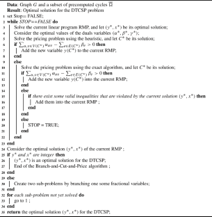
Lift-and-project cuts for convex mixed integer nonlinear programs.

The P vs. NP Problem and Attempts to Settle It via Perfect Graphs State-of-the-Art Approach

Concise integer linear programming formulation for clique partitioning problems
Baïou, M., & Mahjoub, A. R. (1997). Steiner 2-edge connected subgraph polytopes on series-parallel graphs. SIAM Journal on Discrete Mathematics, 10 (3), 505–514.
Article Google Scholar
Barahona, F., & Mahjoub, A. R. (1995). On two connected subgraph polytopes. In Discrete Mathematics , (pp. 19–34).
Ben Salem, M., Hanafi, S., Taktak, R., & Ben-Abdallah, H. (2017). Probabilistic tabu search with multiple neighborhoods for the disjunctively constrained knapsack problem. RAIRO-Operations Research, 51 (3), 627–637.
Ben Salem, M., Taktak, R., Mahjoub, A. R., & Ben-Abdallah, H. (2018). Optimization algorithms for the disjunctively constrained knapsack problem. Soft Computing, 22 (6), 2025–2043.
Bendali, F., Diarrassouba, I., Didi, Biha M., Mailfert, J., & Mahjoub, A. R. (2010). A Branch-and-Cut algorithm for the k-edge connected subgraph problem. Networks, 55 (1), 13–32.
Carrabs, F., Cerulli, R., Pentangelo, R., & Raiconi, A. (2021). Minimum spanning tree with conflicting edge pairs: A branchand-cut approach. Annals of Operations Research, 298 (1), 65–78.
Carrabs, F., & Gaudioso, M. (2021). A lagrangian approach for the minimum spanning tree problem with conflicting edge pairs. Networks, 78 (1), 32–45.
Cplex, I. I. (2020). V12. 9: User’s Manual for CPLEX. International Business Machines Corporation, 46 (53), 157.
Google Scholar
Darmann, A., Pferschy, U., Schauer, J., & Woeginger, G. J. (2011). Paths, trees and matchings under disjunctive constraints. Discrete Applied Mathematics, 159 (16), 1726–1735.
Diarrassouba, I., Mahjoub, A. R., & Kutucu, H. (2013). Two Node-Disjoint Hop-Constrained Survivable Network Design and Polyhedra. In Electronic Notes in Discrete Mathematics , (pp. 551–558).
Diarrassouba, I., Mahjoub, M., Mahjoub, A. R., & Taktak, R. (2016). The k-node connected subgraph problem: Polyhedral analysis and Branch-and-Cut. In Electronic Notes in Discrete Mathematics , (pp. 117–124).
Diarrassouba, I., Mahjoub, M., Mahjoub, A. R., & Yaman, H. (2016). k-node-disjoint hop-constrained survivable networks: polyhedral analysis and branch and cut. In Annals of Telecommunications , (pp. 5–28).
Diarrassouba, I, Mahjoub, M., Mahjoub, A. R., & Taktak, R. (2017). The survivable k-node-connected network design problem: Valid inequalities and Branch-and-Cut. In Computers and Industrial Engineering , (pp. 690–705).
Dixon, E. T., & Goodman, S. E. (1976). An algorithm for the longest cycle problem. In Networks , (pp. 139–149).
Ekici, A. (2021). Bin packing problem with conflicts and item fragmentation. Computers & Operations Research, 126 , 105–113.
Erickson, R. E., Monma, C. L., & Veinott, A. F. (1987). Send-and-Split Method for Minimum-Concave-Cost Network Flows. In Mathematics of Operations Research , (pp. 634–664).
Fortz, B., & Labbé, M. (2002). Polyhedral results for two-connected networks with bounded rings. In Mathematical Programming Journal , (pp. 27–54).
Gamrath, G., Anderson, D., Bestuzheva, K., Chen, W.K., Eifler, L., Gasse, M., Gemander, P., Gleixner, A., Gottwald, L., Halbig, K., and Hendel, G., and Hojny, C., Koch, T., Bodic, L., Maher, P. J., Matter, F., Miltenberger, M., Mühmer, E., Müller, B., Pfetsch, M.E., Schlösser, F., Serrano, F., Shinano, Y., Tawfik, C., Vigerske, S., Wegscheider, F., Weninger, D., & Witzig, J. (2020). The SCIP Optimization Suite 7.0. In Zuse Institute Berlin, March .
Garey, M.R., & Johnson, D.S. (1979). Computers and intractability: A guide to the theory of NP-completeness (series of books in the mathematical sciences) . W. H. Freeman & Co Ltd, First edition.
Goldberg, A.V., & Tarjan, R. E. (1986). A New Approach to the Maximum Flow Problem. In Proceedings of the Eighteenth Annual Association for Computing Machinery Symposium on Theory of Computing , (pp. 136–146).
Grötschel, M., & Monma, C.L. (1990). Integer Polyhedra Arising from Certain Network Design Problems with Connectivity Constraints. In SIAM Journal on Discrete Mathematics , (pp. 502-523).
Grötschel, M., Lovász, L., & Schrijver, A. (2012). Geometric algorithms and combinatorial optimization . Springer Science & Business Media.
Grötschel, M., Monma, C. L., & Stoer, M. (1992). Computational Results with a Cutting Plane Algorithm for Designing Communication Networks with Low-Connectivity Constraints. In Operations Research Journal , (pp. 309–330).
Grötschel, M., Monma, C. L., & Stoer, M. (1992). Facets for Polyhedra Arising in the Design of Communication Networks with Low-Connectivity Constraints. In SIAM Journal on Optimization , (pp. 474–504).
Grötschel, M., Monma, C. L., & Stoer, M. (1995). Polyhedral and computational investigations for designing communication networks with high survivability requirements. Operations Research, 43 , 1012–1024.
Gusfield, D. (1987). Very simple algorithms and programs for all pairs network flow analysis. In Technical report, Computer Science Division , University of California, Davis.
Gusfield, D. (1990). Very simple methods for all pairs network flow analysis. SIAM Journal of Computing, 19 (1), 143–155.
Karp, R. M. (1972). Reducibility among Combinatorial Problems. In Complexity of Computer Computations: Proceedings of a symposium on the Complexity of Computer Computations, held March 20–22, 1972, at the IBM Thomas J. Watson Research Center , (pp. 85–94).
Kerivin, H., & Mahjoub, A. R. (2005). On survivable network polyhedra. In Discrete Mathematics , (pp. 183–210).
Kerivin, H., Mahjoub, A. R., & Nocq, C. (2004). (1,2)-Survivable Networks: Facets and Branch & Cut. In The Sharpest Cut: the Impact of Manfred Padberg and his Work , (pp. 121–152). Mathematical Programming Society : Philadelphia.
Mahjoub, A. R. (1994). Two edge connected spanning subgraphs and polyhedra. In Mathematical Programming , (pp. 199–208).
Mahjoub, A. R. (1997). On Perfectly Two-Edge Connected Graphs. In Discrete Math. , (pp. 153–172). Elsevier Science Publishers B. V.
Mahjoub, A. R. (2010). Polyhedral approaches. In Vangelis Paschos, editor, Concepts of Combinatorial Optimization, ISTE- WIELY , (pp. 261–324).
Mahjoub, M. (2017). The Survivable Network Design Problems with High Node-Connectivity Constraints : Polyhedra and Algorithms. In Theses, Université Paris sciences et lettres , Université de Tunis El Manar.
Mahjoub, A. R., & Nocq, C. (1999). On the linear relaxation of the 2-node connected subgraph polytope. In Discrete Applied Mathematics , (pp. 389–416).
Mahjoub, A. R., & Pesneau, P. (2008). On the Steiner 2-edge connected subgraph polytope. In RAIRO , (pp. 259–283).
Mahjoub, A. R., Poss, M., Simonetti, L., & Uchoa, E. (2019). Distance Transformation for Network Design Problems. In SIAM Journal on Optimization , (pp. 1687–1713).
Mahjoub, A. R., Simonetti, L., & Uchoa, E. (2011). Hop-level flow formulation for the survivable network design with hop constraints problem. In Network optimization book , (pp. 171–179).
Menger, K. (1927). Zur allgemeinen Kurventheorie. Fundamenta Mathematicae, 10 (1), 96–115.
Monma, C. L., Munson, B. S., & Pulleyblank, W. R. (1990). Minimum-weight two-connected spanning networks. Mathematical Programming, 46 , 153–171.
Nemhauser, G. L., & Sigismondi, G. (1992). A Strong Cutting Plane/Branch-and-Bound Algorithm for Node Packing. In The Journal of the Operational Research Society , (pp. 443–457).
Öncan, T., Zhang, R., & Punnen, A. P. (2013). The minimum cost perfect matching problem with conflict pair constraints. Computers & Operations Research, 40 (4), 920–930.
Orlowski, S., Pióro, M., Tomaszewski, A., & Wessäly, R. (2007). SNDlib 1.0-Survivable Network Design Library. In Proceedings of the 3rd International Network Optimization Conference (INOC 2007) . Spa, Belgium.
Padberg, M. W. (1973). On the facial structure of set packing polyhedra. Mathematical Programming, 5 , 199–215.
Pferschy, U., & Schauer, J. (2013). The maximum flow problem with disjunctive constraints. Journal of Combinatorial Optimization, 26 (1), 109–119.
Reinelt, G. (1991). TSPLIB–A Traveling Salesman Problem Library. In ORSA Journal on Computing , (pp. 376–384).
Sadykov, R., & Vanderbeck, F. (2013). Bin packing with conflicts: a generic Branch-and-Price algorithm. INFORMS Journal on Computing, 25 (2), 244–255.
Samer, P., & Urrutia, S. (2015). A branch and cut algorithm for minimum spanning trees under conflict constraints. Optimization Letters, 9 (1), 41–55.
Senisuka, A., You, B., & Yamada, T. (2005). Reduction and exact algorithms for the disjunctively constrained knapsack problem. In International symposium, operational research Bremen . Citeseer.
Şuvak, Z., Altınel, I. K., & Aras, N. (2020). Exact solution algorithms for the maximum flow problem with additional conflict constraints. European Journal of Operational Research, 287 (2), 410–437.
Şuvak, Z., Altınel, I. K., & Aras, N. (2021). Minimum cost flow problem with conflicts. Networks, 78 (4), 421–442.
Talbi, E. G. (2009) Metaheuristics: From Design to Implementation . Wiley Publishing.
Winter, P. (1986). Generalized Steiner Problem in Series-Parallel Networks. In J. Algorithms , (pp. 549–566).
Winter, P. (1987). Steiner Problem in Halin Networks. In Discrete Applied Mathematics , (pp. 281–294).
Winter, P. (1985). Generalized Steiner problem in outerplanar networks. BIT, 25 , 485–496.
Yamada, T., Kataoka, S., & Watanabe, K. (2002). Heuristic and exact algorithms for the disjunctively constrained knapsack problem. Information Processing Society of Japan Journal , 43 (9).
Download references
Author information
Authors and affiliations.
Department of Statistics and Operations Research, College of Science, Kuwait University, Kuwait, Kuwait
Fatmah Almathkour
LMAH, Le Havre Normandie University, Le Havre, France
Ibrahima Diarrassouba
LIMOS, UMR CNRS 6158, Clermont Auvergne INP, 63178, Clermont-Ferrand, France
Youssouf Hadhbi
You can also search for this author in PubMed Google Scholar
Corresponding author
Correspondence to Fatmah Almathkour .
Additional information
Publisher's note.
Springer Nature remains neutral with regard to jurisdictional claims in published maps and institutional affiliations.
Rights and permissions
Springer Nature or its licensor (e.g. a society or other partner) holds exclusive rights to this article under a publishing agreement with the author(s) or other rightsholder(s); author self-archiving of the accepted manuscript version of this article is solely governed by the terms of such publishing agreement and applicable law.
Reprints and permissions
About this article
Almathkour, F., Diarrassouba, I. & Hadhbi, Y. Extended formulation and Branch-and-Cut-and-Price algorithm for the two connected subgraph problem with disjunctive constraints. Ann Oper Res (2024). https://doi.org/10.1007/s10479-024-06123-0
Download citation
Received : 21 July 2023
Accepted : 13 June 2024
Published : 28 June 2024
DOI : https://doi.org/10.1007/s10479-024-06123-0
Share this article
Anyone you share the following link with will be able to read this content:
Sorry, a shareable link is not currently available for this article.
Provided by the Springer Nature SharedIt content-sharing initiative
- Two connected graph
- Disjunctive constraints
- Network design
- Survivability
- Integer programming
- Extended formulation
- Column generation
- Valid inequalities
- Branch-and-Cut-and-Price
- Find a journal
- Publish with us
- Track your research
IMAGES
VIDEO
COMMENTS
An introduction to the basic transportation problem and its linear programming formulation:Transshipment Problem video: https://youtu.be/ABMPgSApdUw Solve Tr...
The transportation problem is a type of Linear Programming problem. In this type of problem, the main objective is to transport goods from source warehouses to various destination locations at minimum cost. In order to solve such problems, we should have demand quantities, supply quantities, and the cost of shipping from source and destination.
Transportation problem is a special kind of Linear Programming Problem (LPP) ... In this article, the method to solve the unbalanced transportation problem will be discussed. Below transportation problem is an unbalanced transportation problem. The problem is unbalanced because the sum of all the supplies i.e. O1 , O2 , O3 and O4 is not equal to t
This essential problem was first formulated as a linear programming problem in the early 1940's and is popularly known as the transportation problem. In this blog, we give an overview of the transportation problem and how the transportation algorithm — as implemented in IMSL — can be used to solve different variations of the ...
The problem of interest is to determine an optimal transportation scheme between the warehouses and the outlets, subject to the specified supply and demand constraints. Graphically, a transportation problem is often visualized as a network with m source nodes, n sink nodes, and a set of m×n "directed arcs." This is depicted in Figure TP-1.
The transportation problem is an important Linear Programming Problem (LPP). This problem depicts the transportation of goods from a group of sources to a group of destinations. The whole process is subject to the availability and demand of the sources as well as destination, respectively in a way, where entire cost of transportation is minimised.
We then define the transportation problem as the linear programming problem of minimize the total transportation cost subject to supply and demand constraints i.e., min x ∑ i = 1 m ∑ j = 1 n c i j x i j s.t. supply constraint : ∑ j = 1 n x i j ≤ S i ∀ i = 1, …, m. demand constraint : ∑ i = 1 m x i j ≥ D j ∀ j = 1, …, n.
In this article, the method to solve the unbalanced transportation problem will be discussed. Below transportation problem is an unbalanced transportation problem. The problem is unbalanced because the sum of all the supplies i.e. O1 , O2 , O3 and O4 is not equal to t ... Transportation problem is a special kind of Linear Programming Problem ...
called the assignment problem. ) We could set up a transportation problem and solve it using the simplex method as with any LP problem (see Using the Simplex Method to Solve Linear Programming Maximization Problems, EM 8720, or another of the sources listed on page 35 for informa-tion about the simplex method). However, the special structure of
The transportation problem. This tutorial was generated using Literate.jl. Download the source as a .jl file. This tutorial was originally contributed by Louis Luangkesorn. This tutorial is an adaptation of the transportation problem described in AMPL: A Modeling Language for Mathematical Programming, by R. Fourer, D.M. Gay and B.W. Kernighan.
Some of the most popular methods are: • Linear Programming: Linear programming techniques have been used to solve the distribution problem, such as the branch-and-cut method. • Heuristic methods: Heuristic methods such as the Clarke-Wright saving algorithm and the Christofides algorithm have been proposed to find approximate ...
The transportation problem deals with a special class of linear programming problems in which the objective is to transport a homogeneous product manufactured at several plants (origins) to a number of different destinations at a minimum total cost. The total supply available at the origin and the total quantity demanded by the destinations are given in the statement of the problem.
To solve a transportation problem, the following information must be given: m= The number of sources. n= The number of destinations. The total quantity available at each source. The total quantity required at each destination. The cost of transportation of one unit of the commodity from each source to each destination.
In this article, the method to solve the unbalanced transportation problem will be discussed. Below transportation problem is an unbalanced transportation problem. The problem is unbalanced because the sum of all the supplies i.e. O1 , O2 , O3 and O4 is not equal to t ... Transportation problem is a special kind of Linear Programming Problem ...
We can solve transportation problems with simplex method, but it will take too much time and very difficult to perform. So we can solve this problem by computer program LINGO or TORA, it is very easy and quick. LINGO or TORA is an interactive computer-software package that can be used to solve linear, integer, and non-linear programming problems.
Cost of transportation is given in terms of 100$ and quantity in tons. Solution: Here , the problem is unbalanced. Now solving the given problem by VAM in single table by calculating penalties for each row and column and assigning maximum amount in minimum cost cell to row/ column with maximum penalty in each round.
The two categories of transportation problems are balanced and unbalanced transportation problems.As we all know, a transportation problem is a type of Linear Programming Problem (LPP) in which items are carried from a set of sources to a set of destinations based on the supply and demand of the sources and destinations, with the goal of minimizing the total transportation cost.
The transportation simplex algorithm is a linear program, a mathematical model representing linear relationships, like the transportation between a supplier and a destination. Linear programming ...
The transportation problem is an extension of linear programming technique because the transportation costs are formulated as a linear function to the supply capacity and demand. Check out the course on transportation analytics. Transportation problem exists in two forms. Balanced.
Running Excel Solver (Linear Programming): When we run the Solver, Solver gives a satisfied solution that states that all the constraints are satisfied. The solution states that we can ship 17 ...
LINGO. 1. Introduction. The transportation problem is a special type of linear programming problem where the objective is to minimise the cost of distributing a product from a number of sources or origins to a number of destinations. Because of its special structure the usual simplex method is not suitable for solving transportation problems.
$\begingroup$ I can solve my problem by writing it as a LP with simplex algorithm. When solving with network simplex I get exactly the trouble which I was afraid of. Following case: totalSupply < totalDemand thus adding a supplyDummy. In the network simplex solution many consumers trade with the added supplyDummy.
A transportation problem in operation research is a special type of Linear Programming Problem used to optimize (minimize) the transportation cost and allocate resources from M source to N destination. This article will briefly discuss transportation problems, types of transportation problems, and how to solve them.
This article takes on two titans of operations research: George Dantzig and Richard Bellman. Those in the O.R. community will immediately recognize Dantzig's contribution of the simplex algorithm for solving linear programs and Bellman's contribution of "Bellman's equation" for solving sequential decision problems that he called "dynamic programs." However, very few people need ...
First, we give an extended formulation for the problem whose variables are the cycles of the graph. Then, we use a column generation algorithm to solve its linear relaxation, and further show that the pricing reduces to finding a specific cycle in the graph which can be formulated as an integer programming problem.
CDK Global says it will likely take several days for its software to be back online and operational, as the company grapples with a system outage that has paralyzed thousands of auto dealerships ...