solving rate of change problems

• Derivatives

How to Find Average Rates of Change: Practice Problems

more interesting facts

more about imaginary numbers

Determine the average rate of change for $$\displaystyle f(x) = \frac{x+1}{x+2}$$ from $$x = 0$$ to $$x = 4$$ .

Calculate the average rate of change .

$$ \begin{align*} \frac{\Delta f}{\Delta x} & = \frac{\blue{f(4)} - \red{f(0)}}{4 - 0}\\[6pt] & = \frac{\blue{\frac{4+1}{4+2}} - \red{\frac{0+1}{0+2}}} 4\\[6pt] & = \frac{\blue{\frac 5 6} - \red{\frac 1 2}} 4\\[6pt] & = \frac{1/3} 4\\[6pt] & = \frac 1 {12} \end{align*} $$

$$\displaystyle \frac{\Delta f}{\Delta x} = \frac 1 {12}$$

Determine the average rate of change for $$f(x) = \sin x$$ from $$x = \pi$$ to $$x = 2\pi$$ (where $$x$$ is measured in radians).

$$ \begin{align*} \frac{\Delta f}{\Delta x} & = \frac{\blue{f(2\pi)}-\red{f(\pi)}}{2\pi - \pi}\\[6pt] & = \frac{\blue{\sin 2\pi}-\red{\sin\pi}}{\pi}\\[6pt] & = \frac{\blue{0}-\red{0}}{\pi}\\[6pt] & = 0 \end{align*} $$

$$\displaystyle \frac{\Delta f}{\Delta x} = 0$$

Determine the average rate of change for the function below, from $$t = -2$$ to $$t = 8$$ .

$$ f(x) = 60e^{0.5t} $$

$$ \begin{align*} \frac{\Delta f}{\Delta t} & = \frac{\blue{f(8)} - \red{f(-2)}}{8 - (-2)}\\[6pt] & = \frac{\blue{60e^{0.5(8)}} - \red{60e^{0.5(-2)}}}{8 - (-2)}\\[6pt] & = \frac{60\left(e^4 - e^{-1}\right)}{10}\\[6pt] & = 6\left(e^4 - e^{-1}\right)\\[6pt] & \approx 325.3816 \end{align*} $$

$$ \displaystyle \frac{\Delta f}{\Delta t} = 6\left(e^4 - e^{-1}\right)\approx 325.3816 $$

Determine the average rate of change for the function below, from $$x = -6$$ to $$x = -3$$ .

$$ f(x) = 2 - 8x - 5x^3 $$

$$ \begin{align*} \frac{\Delta f}{\Delta x} & = \frac{\blue{f(-3)} - \red{f(-6)}}{-3 - (-6)}\\[6pt] & = \frac{\blue{(2 - 8(-3) - 5(-3)^3)} - \red{(2 - 8(-6) - 5(-6)^3)}}{-3 +6}\\[6pt] & = \frac{\blue{161} - \red{1130}} 3\\[6pt] & = -\frac{969} 3\\[6pt] & = - 323 \end{align*} $$

$$\frac{\Delta f}{\Delta x} = -323$$

Suppose the average size of a particular population of cute, fluffy bunny rabbits can be described by the function

$$ P(t) = \frac{250}{1+4e^{-0.75t}}, $$

where $$t$$ is measured in years and $$P(t)$$ is measured in numbers of bunnies.

As time increases from $$t = 5$$ to $$t = 10$$ , what is the average rate of change in the bunny population?

$$ \begin{align*} \frac{\Delta P}{\Delta t} & = \frac{\blue{P(10)} - \red{P(5)}}{10 -5}\\[6pt] & = \frac{\blue{\frac{250}{1+4e^{-0.75(10)}}} - \red{\frac{250}{1+4e^{-0.75(5)}}}}{5}\\[6pt] & = \frac{250\left(\frac 1 {1+4e^{-7.5}} - \frac 1 {1+4e^{-3.75}}\right)}{5}\\[6pt] & = 50\left(\frac 1 {1+4e^{-7.5}} - \frac 1 {1+4e^{-3.75}}\right)\\[6pt] & \approx 4.2 \end{align*} $$

From year 5 to year 10 the population of cute, fluffy bunnies increases at an average rate of about 4.2 bunnies per year.

At a particular company, the cost of producing $$x$$ pallets of goods can be described by the function

$$ C(x) = 25x + 4500, $$

where $$C(x)$$ is measured in dollars. Determine the average rate of change in the cost as production decreases from 150 pallets to 120 pallets.

$$ \begin{align*} \frac{\Delta C}{\Delta x} & = \frac{\blue{C(120)} - \red{C(150)}}{120 - 150}\\[6pt] & = \frac{\blue{25(120)+4500} - \red{25(150)+4500}}{-30}\\[6pt] & = \frac{\blue{7500} - \red{8250}}{-30}\\[6pt] & = \frac{-750}{-30}\\ & = 25 \end{align*} $$

As the amount of goods produced drops from 150 pallets to 120 pallets, the cost of production decreases an average of $25 per pallet.

Note 1: We could have saved ourselves the effort of calculating $$\Delta C/\Delta x$$ by simply noticing $$C(x)$$ is a linear function. The average rate of change of any linear function is just its slope.

Note 2: When the average rate of change is positive, the function and the variable will change in the same direction. In this case, since the amount of goods being produced decreases, so does the cost.

Suppose you invest $2000 in an account that earns 8% interest each year, but interest is compounded each month. Then the amount you have in the account is described by the function

$$ A(t) = 2000\left(1 + \frac{0.08}{12}\right)^{12t}. $$

If you make no deposits or withdrawals, what is the average rate of change in the amount of money in the account ...

• over the first 5 years?
• over the second 5 years?

$$ \begin{align*} \frac{\Delta A}{\Delta t} & = \frac{\blue{A(5)} - \red{A(0)}}{5-0}\\[6pt] & = \frac{\blue{2000\left(1 + \frac{0.08}{12}\right)^{12(5)}} - \red{2000\left(1 + \frac{0.08}{12}\right)^{12(0)}}}{5}\\[6pt] & = \blue{400\left(1 + \frac{0.08}{12}\right)^{60}} - \red{400\left(1 + \frac{0.08}{12}\right)^{0}}\\[6pt] & = \blue{400\left(1 + \frac{0.08}{12}\right)^{60}} - \red{400}\\[6pt] & \approx 195.94 \end{align*} $$

$$ \begin{align*} \frac{\Delta A}{\Delta t} & = \frac{\blue{A(10)} - \red{A(5)}}{10-5}\\[6pt] & = \frac{\blue{2000\left(1 + \frac{0.08}{12}\right)^{12(10)}} - \red{2000\left(1 + \frac{0.08}{12}\right)^{12(5)}}} 5\\[6pt] & = \blue{400\left(1 + \frac{0.08}{12}\right)^{120}} - \red{400\left(1 + \frac{0.08}{12}\right)^{60}}\\[6pt] & \approx 291.92 \end{align*} $$

• During the first five years, the account grows by an average of $195.94 per year.
• During the second five years, the account grows by an average of $291.92 per year.

Suppose a particular electrical circuit is designed to keep the current, $$I$$, at a constant $$0.02$$ amps. However, both the voltage, $$V$$, and the resistance, $$R$$, can vary. Then according to Ohm's Law,

$$R = \frac{0.02} V,$$

where $$R$$ is measured in Ohms and $$V$$ is measured in volts.

What is the average rate of change in the resistance on the circuit as the voltage increases from 1.5 volts to 9 volts?

$$ \begin{align*} \frac{\Delta R}{\Delta V} & = \frac{\blue{R(9)}-\red{R(1.5)}}{9-1.5}\\[6pt] & = \frac{\blue{\frac{0.02} 9}-\red{\frac{0.02}{1.5}}}{7.5}\\[6pt] & = \left(\blue{\frac{0.02} 9}-\red{\frac{0.02}{1.5}}\right)\cdot \frac 1 {7.5}\\[6pt] & = -\frac 1 {675}\\[6pt] & \approx -0.00148 \end{align*} $$

As the voltage increases from 1.5 volts to 9 volts the resistance will decrease at an average rate of $$\frac 1 {675}$$ ohms per volt, or approximately 0.00148 ohms per volt.

Suppose $$P(t)$$ represents the proficiency achieved at a particular task after receiving $$t$$ hours training. Suppose the following equation applies when $$t$$ increases from 3 to 12. Interpret the equation in a complete sentence.

$$ \frac{\Delta P}{\Delta t} = 12\% $$

Rewrite the average rate of change as a fraction with a denominator of 1.

$$ \frac{\Delta P}{\Delta t} = 12\% = \frac{12\%} 1 $$

As $$t$$ increases from 3 hours to 12 hours of training, proficiency increases at an average rate of 12% per hour.

Suppose $$R(x)$$ represents the revenue (in thousands of dollars) earned by a particular company from the sale of $$x$$ tons of goods. Suppose the following equation applies when sales increase from 0.8 tons to 1.4 tons. Interpret the equation in a complete sentence.

$$ \frac{\Delta R}{\Delta x} = -0.2 $$

Rewrite the average rate of change so it has a 1 in the denominator.

$$ \frac{\Delta R}{\Delta x} = -0.2 = -\frac{0.2} 1 $$

When sales increase from 0.8 to 1.4 tons, the company's revenue decreases at an average rate of $200 per ton of goods sold.

Note 1: Since the average rate of change is negative, the two quantities change in opposite directions. Since the amount of goods sold is increasing, revenue must be decreasing. Note 2: Even though the average rate of change in revenue is negative, this does not mean that the company is losing money. It only means they are earning less per ton than previously. This might happen if the company decreases the price of their goods. They sell more goods, but earn less per item.

Suppose the current in an electrical circuit increases at an average rate of 0.03 amps per second. Write an equation expressing this idea.

Define variables.

• Let $$I = $$ the amount of electrical current flowing through the circuit, measured in amps.
• Let $$t$$ represent time, measured in seconds.

$$\displaystyle \frac{\Delta I}{\Delta t} = 0.03$$

Suppose someone drives with an average velocity of 85 kilometers per hour. Write an equation expressing this idea.

• Let $$d$$ represent the persons distance from their starting point, in kilometers.
• Let $$t$$ represent time, in hours.

$$\displaystyle \frac{\Delta d}{\Delta t} = 85$$

Suppose someone has been driving for 45 minutes at a steady 50 kilometers per hour. Then they increased their speed and drove for the another 1.5 hours. When they arrived at their destination, their average speed for the entire trip was 80 kilometers per hour. How fast did they drive during the last 1.5 hours?

Find the total distance driven if the person had been driving at 80 kph for the entire 2.25 hours.

$$ \frac{80\mbox{ kilometers}}{1\mbox{ hour}} \cdot \frac{2.25\mbox{ hours}} 1 = (80)(2.25) \mbox{ kilometers} = 180 kilometers $$

Determine the remaining distance that had to be driven during the last 1.5 hours.

The driver has spent $$3/4$$ of an hour driving at 50 kph, and so had traveled $$50\cdot 0.75 = 37.5$$ kilometers. This left $$180-37.5 = 142.5$$ kilometers to travel.

Determine the speed needed to cover the remaining distance in the remaining time.

The person needed to travel 142.5 kilometers in 1.5 hours. So the speed had to be

$$ \frac{142.5\mbox{ kilometers}}{1.5\mbox{ hours}} = 95\mbox{ kph.} $$

The person drove at a speed of 95 kilometers per hour for the last 1.5 hours.

In electrical circuits, energy is measured in joules (pronounced jools ) and power is measured in watts. The relationship between the two is

$$ 1\mbox{ watt} = \frac {1\mbox{ joule}}{\mbox{second}} $$

So, watts are the rate of change of energy relative to time (just like speed is the rate of change of distance relative to time).

Suppose a variable wattage lightbulb (like a lightbulb on a dimmer switch) has been pulling 30 watts for the past 15 minutes. The wattage is then increased so that after another 5 minutes the average rate of change for the entire 20 minutes is 50 watts.

What was the higher wattage the bulb was set to in order to achieve this?

Determine the total amount of energy used during the 20 minutes.

$$ \frac{50\mbox{ joules}}{\mbox{second}} \cdot \frac{20\mbox{ minutes}} 1 = \frac{50\mbox{ joules}}{\mbox{second}} \cdot \frac{1200\mbox{ seconds}} 1 = 60{,}000\mbox{ joules}. $$

Determine the amount of energy that needed to be used during the last 5 minutes.

Since the bulb had been burning at 30 watts for 15 minutes, it had already used

$$ \frac{30\mbox{ joules}}{\mbox{second}} \cdot \frac{15\mbox{ minutes}} 1 = \frac{30\mbox{ joules}}{\mbox{second}} \cdot \frac{900 \mbox{ seconds}} 1 = 27{,}000\mbox{ joules}. $$

The remaining energy to be used would be 60,000-27,000=33,000 joules.

Determine the rate (in joules/second) that would be needed to use the remaining energy during the last 5 minutes.

The remaining energy would have to be used in 5 minutes which is the same as 300 seconds. So, we have

$$ \frac{33{,}000\mbox{ joules}}{300\mbox{ seconds}} = \frac{110\mbox{ joules}}{1\mbox{ second}} = 110\mbox{ watts}. $$

The bulb would have burned at 110 watts during the last 5 minutes.

Ultimate Math Solver (Free)

Free Algebra Solver ... type anything in there!

Popular pages @ mathwarehouse.com and around the web

HIGH SCHOOL

• ACT Tutoring
• SAT Tutoring
• PSAT Tutoring
• ASPIRE Tutoring
• SHSAT Tutoring
• STAAR Tutoring

GRADUATE SCHOOL

• MCAT Tutoring
• GRE Tutoring
• LSAT Tutoring
• GMAT Tutoring
• AIMS Tutoring
• HSPT Tutoring
• ISAT Tutoring
• SSAT Tutoring

Search 50+ Tests

Loading Page

math tutoring

• Elementary Math
• Pre-Calculus
• Trigonometry

science tutoring

Foreign languages.

• Mandarin Chinese

elementary tutoring

• Computer Science

Search 350+ Subjects

• Video Overview
• Tutor Selection Process
• Online Tutoring
• Mobile Tutoring
• Instant Tutoring
• How We Operate
• Our Guarantee
• Impact of Tutoring
• Reviews & Testimonials
• About Varsity Tutors

Precalculus : Rate of Change Problems

Study concepts, example questions & explanations for precalculus, all precalculus resources, example questions, example question #1 : rate of change problems.

Example Question #2 : Rate Of Change Problems

Example Question #3 : Rate Of Change Problems

Find the average rate of change in profit when production increases from 4 items to 5 items.

Find the average rate of change in demand when the price increases from $2 per treat to $3 per treat.

This implies that the demand drops as the price increases.

Example Question #10 : Rate Of Change Problems

Report an issue with this question

If you've found an issue with this question, please let us know. With the help of the community we can continue to improve our educational resources.

DMCA Complaint

If you believe that content available by means of the Website (as defined in our Terms of Service) infringes one or more of your copyrights, please notify us by providing a written notice (“Infringement Notice”) containing the information described below to the designated agent listed below. If Varsity Tutors takes action in response to an Infringement Notice, it will make a good faith attempt to contact the party that made such content available by means of the most recent email address, if any, provided by such party to Varsity Tutors.

Your Infringement Notice may be forwarded to the party that made the content available or to third parties such as ChillingEffects.org.

Please be advised that you will be liable for damages (including costs and attorneys’ fees) if you materially misrepresent that a product or activity is infringing your copyrights. Thus, if you are not sure content located on or linked-to by the Website infringes your copyright, you should consider first contacting an attorney.

Please follow these steps to file a notice:

You must include the following:

A physical or electronic signature of the copyright owner or a person authorized to act on their behalf; An identification of the copyright claimed to have been infringed; A description of the nature and exact location of the content that you claim to infringe your copyright, in \ sufficient detail to permit Varsity Tutors to find and positively identify that content; for example we require a link to the specific question (not just the name of the question) that contains the content and a description of which specific portion of the question – an image, a link, the text, etc – your complaint refers to; Your name, address, telephone number and email address; and A statement by you: (a) that you believe in good faith that the use of the content that you claim to infringe your copyright is not authorized by law, or by the copyright owner or such owner’s agent; (b) that all of the information contained in your Infringement Notice is accurate, and (c) under penalty of perjury, that you are either the copyright owner or a person authorized to act on their behalf.

Send your complaint to our designated agent at:

Charles Cohn Varsity Tutors LLC 101 S. Hanley Rd, Suite 300 St. Louis, MO 63105

Or fill out the form below:

Contact Information

Complaint details.

3.4 Derivatives as Rates of Change

Learning objectives.

• 3.4.1 Determine a new value of a quantity from the old value and the amount of change.
• 3.4.2 Calculate the average rate of change and explain how it differs from the instantaneous rate of change.
• 3.4.3 Apply rates of change to displacement, velocity, and acceleration of an object moving along a straight line.
• 3.4.4 Predict the future population from the present value and the population growth rate.
• 3.4.5 Use derivatives to calculate marginal cost and revenue in a business situation.

In this section we look at some applications of the derivative by focusing on the interpretation of the derivative as the rate of change of a function. These applications include acceleration and velocity in physics, population growth rates in biology, and marginal functions in economics.

Amount of Change Formula

One application for derivatives is to estimate an unknown value of a function at a point by using a known value of a function at some given point together with its rate of change at the given point. If f ( x ) f ( x ) is a function defined on an interval [ a , a + h ] , [ a , a + h ] , then the amount of change of f ( x ) f ( x ) over the interval is the change in the y y values of the function over that interval and is given by

The average rate of change of the function f f over that same interval is the ratio of the amount of change over that interval to the corresponding change in the x x values. It is given by

As we already know, the instantaneous rate of change of f ( x ) f ( x ) at a a is its derivative

For small enough values of h , f ′ ( a ) ≈ f ( a + h ) − f ( a ) h . h , f ′ ( a ) ≈ f ( a + h ) − f ( a ) h . We can then solve for f ( a + h ) f ( a + h ) to get the amount of change formula:

We can use this formula if we know only f ( a ) f ( a ) and f ′ ( a ) f ′ ( a ) and wish to estimate the value of f ( a + h ) . f ( a + h ) . For example, we may use the current population of a city and the rate at which it is growing to estimate its population in the near future. As we can see in Figure 3.22 , we are approximating f ( a + h ) f ( a + h ) by the y y coordinate at a + h a + h on the line tangent to f ( x ) f ( x ) at x = a . x = a . Observe that the accuracy of this estimate depends on the value of h h as well as the value of f ′ ( a ) . f ′ ( a ) .

Here is an interesting demonstration of rate of change.

Example 3.33

Estimating the value of a function.

If f ( 3 ) = 2 f ( 3 ) = 2 and f ′ ( 3 ) = 5 , f ′ ( 3 ) = 5 , estimate f ( 3.2 ) . f ( 3.2 ) .

Begin by finding h . h . We have h = 3.2 − 3 = 0.2 . h = 3.2 − 3 = 0.2 . Thus,

Checkpoint 3.21

Given f ( 10 ) = −5 f ( 10 ) = −5 and f ′ ( 10 ) = 6 , f ′ ( 10 ) = 6 , estimate f ( 10.1 ) . f ( 10.1 ) .

Motion along a Line

Another use for the derivative is to analyze motion along a line. We have described velocity as the rate of change of position. If we take the derivative of the velocity, we can find the acceleration, or the rate of change of velocity. It is also important to introduce the idea of speed , which is the magnitude of velocity. Thus, we can state the following mathematical definitions.

Let s ( t ) s ( t ) be a function giving the position of an object at time t . t .

The velocity of the object at time t t is given by v ( t ) = s ′ ( t ) . v ( t ) = s ′ ( t ) .

The speed of the object at time t t is given by | v ( t ) | . | v ( t ) | .

The acceleration of the object at t t is given by a ( t ) = v ′ ( t ) = s ″ ( t ) . a ( t ) = v ′ ( t ) = s ″ ( t ) .

Example 3.34

Comparing instantaneous velocity and average velocity.

A ball is dropped from a height of 64 feet. Its height above ground (in feet) t t seconds later is given by s ( t ) = −16 t 2 + 64 . s ( t ) = −16 t 2 + 64 .

• What is the instantaneous velocity of the ball when it hits the ground?
• What is the average velocity during its fall?

The first thing to do is determine how long it takes the ball to reach the ground. To do this, set s ( t ) = 0 . s ( t ) = 0 . Solving −16 t 2 + 64 = 0 , −16 t 2 + 64 = 0 , we get t = 2 , t = 2 , so it take 2 seconds for the ball to reach the ground.

• The instantaneous velocity of the ball as it strikes the ground is v ( 2 ) . v ( 2 ) . Since v ( t ) = s ′ ( t ) = −32 t , v ( t ) = s ′ ( t ) = −32 t , we obtain v ( t ) = −64 ft/s . v ( t ) = −64 ft/s .
• The average velocity of the ball during its fall is v a v e = s ( 2 ) − s ( 0 ) 2 − 0 = 0 − 64 2 = −32 ft/s . v a v e = s ( 2 ) − s ( 0 ) 2 − 0 = 0 − 64 2 = −32 ft/s .

Example 3.35

Interpreting the relationship between v ( t ) v ( t ) and a ( t ) a ( t ).

A particle moves along a coordinate axis in the positive direction to the right. Its position at time t t is given by s ( t ) = t 3 − 4 t + 2 . s ( t ) = t 3 − 4 t + 2 . Find v ( 1 ) v ( 1 ) and a ( 1 ) a ( 1 ) and use these values to answer the following questions.

• Is the particle moving from left to right or from right to left at time t = 1 ? t = 1 ?
• Is the particle speeding up or slowing down at time t = 1 ? t = 1 ?

Begin by finding v ( t ) v ( t ) and a ( t ) . a ( t ) .

v ( t ) = s ′ ( t ) = 3 t 2 - 4 v ( t ) = s ′ ( t ) = 3 t 2 - 4 and a ( t ) = v ′ ( t ) = s ″ ( t ) = 6 t . a ( t ) = v ′ ( t ) = s ″ ( t ) = 6 t .

Evaluating these functions at t = 1 , t = 1 , we obtain v ( 1 ) = −1 v ( 1 ) = −1 and a ( 1 ) = 6 . a ( 1 ) = 6 .

• Because v ( 1 ) < 0 , v ( 1 ) < 0 , the particle is moving from right to left.
• Because v ( 1 ) < 0 v ( 1 ) < 0 and a ( 1 ) > 0 , a ( 1 ) > 0 , velocity and acceleration are acting in opposite directions. In other words, the particle is being accelerated in the direction opposite the direction in which it is traveling, causing | v ( t ) | | v ( t ) | to decrease. The particle is slowing down.

Example 3.36

Position and velocity.

The position of a particle moving along a coordinate axis is given by s ( t ) = t 3 − 9 t 2 + 24 t + 4 , t ≥ 0 . s ( t ) = t 3 − 9 t 2 + 24 t + 4 , t ≥ 0 .

• Find v ( t ) . v ( t ) .
• At what time(s) is the particle at rest?
• On what time intervals is the particle moving from left to right? From right to left?
• Use the information obtained to sketch the path of the particle along a coordinate axis.
• The velocity is the derivative of the position function: v ( t ) = s ′ ( t ) = 3 t 2 − 18 t + 24 . v ( t ) = s ′ ( t ) = 3 t 2 − 18 t + 24 .
• The particle is at rest when v ( t ) = 0 , v ( t ) = 0 , so set 3 t 2 − 18 t + 24 = 0 . 3 t 2 − 18 t + 24 = 0 . Factoring the left-hand side of the equation produces 3 ( t − 2 ) ( t − 4 ) = 0 . 3 ( t − 2 ) ( t − 4 ) = 0 . Solving, we find that the particle is at rest at t = 2 t = 2 and t = 4 . t = 4 .

Checkpoint 3.22

A particle moves along a coordinate axis. Its position at time t t is given by s ( t ) = t 2 − 5 t + 1 . s ( t ) = t 2 − 5 t + 1 . Is the particle moving from right to left or from left to right at time t = 3 ? t = 3 ?

Population Change

In addition to analyzing velocity, speed, acceleration, and position, we can use derivatives to analyze various types of populations, including those as diverse as bacteria colonies and cities. We can use a current population, together with a growth rate, to estimate the size of a population in the future. The population growth rate is the rate of change of a population and consequently can be represented by the derivative of the size of the population.

If P ( t ) P ( t ) is the number of entities present in a population, then the population growth rate of P ( t ) P ( t ) is defined to be P ′ ( t ) . P ′ ( t ) .

Example 3.37

Estimating a population.

The population of a city is tripling every 5 years. If its current population is 10,000, what will be its approximate population 2 years from now?

Let P ( t ) P ( t ) be the population (in thousands) t t years from now. Thus, we know that P ( 0 ) = 10 P ( 0 ) = 10 and based on the information, we anticipate P ( 5 ) = 30 . P ( 5 ) = 30 . Now estimate P ′ ( 0 ) , P ′ ( 0 ) , the current growth rate, using

By applying Equation 3.10 to P ( t ) , P ( t ) , we can estimate the population 2 years from now by writing

thus, in 2 years the population will be 18,000.

Checkpoint 3.23

The current population of a mosquito colony is known to be 3,000; that is, P ( 0 ) = 3,000 . P ( 0 ) = 3,000 . If P ′ ( 0 ) = 100 , P ′ ( 0 ) = 100 , estimate the size of the population in 3 days, where t t is measured in days.

Changes in Cost and Revenue

In addition to analyzing motion along a line and population growth, derivatives are useful in analyzing changes in cost, revenue, and profit. The concept of a marginal function is common in the fields of business and economics and implies the use of derivatives. The marginal cost is the derivative of the cost function. The marginal revenue is the derivative of the revenue function. The marginal profit is the derivative of the profit function, which is based on the cost function and the revenue function.

If C ( x ) C ( x ) is the cost of producing x items, then the marginal cost M C ( x ) M C ( x ) is M C ( x ) = C ′ ( x ) . M C ( x ) = C ′ ( x ) .

If R ( x ) R ( x ) is the revenue obtained from selling x x items, then the marginal revenue M R ( x ) M R ( x ) is M R ( x ) = R ′ ( x ) . M R ( x ) = R ′ ( x ) .

If P ( x ) = R ( x ) − C ( x ) P ( x ) = R ( x ) − C ( x ) is the profit obtained from selling x items, then the marginal profit M P ( x ) M P ( x ) is defined to be M P ( x ) = P ′ ( x ) = M R ( x ) − M C ( x ) = R ′ ( x ) − C ′ ( x ) . M P ( x ) = P ′ ( x ) = M R ( x ) − M C ( x ) = R ′ ( x ) − C ′ ( x ) .

We can roughly approximate

by choosing an appropriate value for h . h . Since x represents objects, a reasonable and small value for h h is 1. Thus, by substituting h = 1 , h = 1 , we get the approximation M C ( x ) = C ′ ( x ) ≈ C ( x + 1 ) − C ( x ) . M C ( x ) = C ′ ( x ) ≈ C ( x + 1 ) − C ( x ) . Consequently, C ′ ( x ) C ′ ( x ) for a given value of x x can be thought of as the change in cost associated with producing one additional item. In a similar way, M R ( x ) = R ′ ( x ) M R ( x ) = R ′ ( x ) approximates the revenue obtained by selling one additional item, and M P ( x ) = P ′ ( x ) M P ( x ) = P ′ ( x ) approximates the profit obtained by producing and selling one additional item.

Example 3.38

Applying marginal revenue.

Assume that the number of barbeque dinners that can be sold, x , x , can be related to the price charged, p , p , by the equation p ( x ) = 9 − 0.03 x , 0 ≤ x ≤ 300 . p ( x ) = 9 − 0.03 x , 0 ≤ x ≤ 300 .

In this case, the revenue in dollars obtained by selling x x barbeque dinners is given by

Use the marginal revenue function to estimate the revenue obtained from selling the 101st barbeque dinner. Compare this to the actual revenue obtained from the sale of this dinner.

First, find the marginal revenue function: M R ( x ) = R ′ ( x ) = −0.06 x + 9 . M R ( x ) = R ′ ( x ) = −0.06 x + 9 .

Next, use R ′ ( 100 ) R ′ ( 100 ) to approximate R ( 101 ) − R ( 100 ) , R ( 101 ) − R ( 100 ) , the revenue obtained from the sale of the 101st dinner. Since R ′ ( 100 ) = 3 , R ′ ( 100 ) = 3 , the revenue obtained from the sale of the 101st dinner is approximately $3.

The actual revenue obtained from the sale of the 101st dinner is

The marginal revenue is a fairly good estimate in this case and has the advantage of being easy to compute.

Checkpoint 3.24

Suppose that the profit obtained from the sale of x x fish-fry dinners is given by P ( x ) = −0.03 x 2 + 8 x − 50 . P ( x ) = −0.03 x 2 + 8 x − 50 . Use the marginal profit function to estimate the profit from the sale of the 101st fish-fry dinner.

Section 3.4 Exercises

For the following exercises, the given functions represent the position of a particle traveling along a horizontal line; t ≥ 0 t ≥ 0 .

• Find the velocity and acceleration functions.
• Determine the time intervals when the object is slowing down or speeding up.

s ( t ) = 2 t 3 − 3 t 2 − 12 t + 8 s ( t ) = 2 t 3 − 3 t 2 − 12 t + 8

s ( t ) = 2 t 3 − 15 t 2 + 36 t − 10 s ( t ) = 2 t 3 − 15 t 2 + 36 t − 10

s ( t ) = t 1 + t 2 s ( t ) = t 1 + t 2

A model rocket is fired vertically upward from the ground. The distance s s in feet that the rocket travels from the ground after t t seconds is given by s ( t ) = −16 t 2 + 560 t . s ( t ) = −16 t 2 + 560 t .

• Find the velocity of the rocket 3 seconds after being fired.
• Find the acceleration of the rocket 3 seconds after being fired.

A ball is thrown downward with a speed of 8 ft/s from the top of a 64-foot-tall building. After t seconds, its height above the ground is given by s ( t ) = −16 t 2 − 8 t + 64 . s ( t ) = −16 t 2 − 8 t + 64 .

• Determine how long it takes for the ball to hit the ground.
• Determine the velocity of the ball when it hits the ground.

The position function s ( t ) = t 2 − 3 t − 4 s ( t ) = t 2 − 3 t − 4 represents the position of the back of a car backing out of a driveway and then driving in a straight line, where s s is in feet and t t is in seconds. In this case, s ( t ) = 0 s ( t ) = 0 represents the time at which the back of the car is at the garage door, so s ( 0 ) = −4 s ( 0 ) = −4 is the starting position of the car, 4 feet inside the garage.

• Determine the velocity of the car when s ( t ) = 0 . s ( t ) = 0 .
• Determine the velocity of the car when s ( t ) = 14 . s ( t ) = 14 .

The position of a hummingbird flying along a straight line in t t seconds is given by s ( t ) = 3 t 3 − 7 t s ( t ) = 3 t 3 − 7 t meters.

• Determine the velocity of the bird at t = 1 t = 1 sec.
• Determine the acceleration of the bird at t = 1 t = 1 sec.
• Determine the acceleration of the bird when the velocity equals 0.

A potato is launched vertically upward with an initial velocity of 100 ft/s from a potato gun at the top of an 85-foot-tall building. The position of the potato relative to the ground after t t seconds is given by s ( t ) = −16 t 2 + 100 t + 85 . s ( t ) = −16 t 2 + 100 t + 85 .

• Find the velocity of the potato after 0.5 s 0.5 s and 5.75 s . 5.75 s .
• Find the speed of the potato at 0.5 s and 5.75 s.
• Determine when the potato reaches its maximum height.
• Find the acceleration of the potato at 0.5 s and 1.5 s.
• Determine how long the potato is in the air.
• Determine the velocity of the potato upon hitting the ground.

The position function s ( t ) = t 3 − 8 t s ( t ) = t 3 − 8 t gives the position in miles of a freight train where east is the positive direction and t t is measured in hours.

• Determine the direction the train is traveling when s ( t ) = 0 . s ( t ) = 0 .
• Determine the direction the train is traveling when a ( t ) = 0 . a ( t ) = 0 .
• Determine the time intervals when the train is slowing down or speeding up.

The following graph shows the position y = s ( t ) y = s ( t ) of an object moving along a straight line.

• Use the graph of the position function to determine the time intervals when the velocity is positive, negative, or zero.
• Sketch the graph of the velocity function.
• Use the graph of the velocity function to determine the time intervals when the acceleration is positive, negative, or zero.
• Determine the time intervals when the object is speeding up or slowing down.

The cost function, in dollars, of a company that manufactures food processors is given by C ( x ) = 200 + 7 x + x 2 7 , C ( x ) = 200 + 7 x + x 2 7 , where x x is the number of food processors manufactured.

• Find the marginal cost function.
• Use the marginal cost function to estimate the cost of manufacturing the thirteenth food processor.
• Find the actual cost of manufacturing the thirteenth food processor.

The price p p (in dollars) and the demand x x for a certain digital clock radio is given by the price–demand function p = 10 − 0.001 x . p = 10 − 0.001 x .

• Find the revenue function R ( x ) . R ( x ) .
• Find the marginal revenue function.
• Find the marginal revenue at x = 2000 x = 2000 and 5000 . 5000 .

[T] A profit is earned when revenue exceeds cost. Suppose the profit function for a skateboard manufacturer is given by P ( x ) = 30 x − 0.3 x 2 − 250 , P ( x ) = 30 x − 0.3 x 2 − 250 , where x x is the number of skateboards sold.

• Find the exact profit from the sale of the thirtieth skateboard.
• Find the marginal profit function and use it to estimate the profit from the sale of the thirtieth skateboard.

[T] In general, the profit function is the difference between the revenue and cost functions: P ( x ) = R ( x ) − C ( x ) . P ( x ) = R ( x ) − C ( x ) .

Suppose the price-demand and cost functions for the production of cordless drills is given respectively by p = 143 − 0.03 x p = 143 − 0.03 x and C ( x ) = 75,000 + 65 x , C ( x ) = 75,000 + 65 x , where x x is the number of cordless drills that are sold at a price of p p dollars per drill and C ( x ) C ( x ) is the cost of producing x x cordless drills.

• Find the revenue and marginal revenue functions.
• Find R ′ ( 1000 ) R ′ ( 1000 ) and R ′ ( 4000 ) . R ′ ( 4000 ) . Interpret the results.
• Find the profit and marginal profit functions.
• Find P ′ ( 1000 ) P ′ ( 1000 ) and P ′ ( 4000 ) . P ′ ( 4000 ) . Interpret the results.

A small town in Ohio commissioned an actuarial firm to conduct a study that modeled the rate of change of the town’s population. The study found that the town’s population (measured in thousands of people) can be modeled by the function P ( t ) = − 1 3 t 3 + 64 t + 3000 , P ( t ) = − 1 3 t 3 + 64 t + 3000 , where t t is measured in years.

• Find the rate of change function P ′ ( t ) P ′ ( t ) of the population function.
• Find P ′ ( 1 ) , P ′ ( 2 ) , P ′ ( 3 ) , P ′ ( 1 ) , P ′ ( 2 ) , P ′ ( 3 ) , and P ′ ( 4 ) . P ′ ( 4 ) . Interpret what the results mean for the town.
• Find P ″ ( 1 ) , P ″ ( 2 ) , P ″ ( 3 ) , P ″ ( 1 ) , P ″ ( 2 ) , P ″ ( 3 ) , and P ″ ( 4 ) . P ″ ( 4 ) . Interpret what the results mean for the town’s population.

[T] A culture of bacteria grows in number according to the function N ( t ) = 3000 ( 1 + 4 t t 2 + 100 ) , N ( t ) = 3000 ( 1 + 4 t t 2 + 100 ) , where t t is measured in hours.

• Find the rate of change of the number of bacteria.
• Find N ′ ( 0 ) , N ′ ( 10 ) , N ′ ( 20 ) , N ′ ( 0 ) , N ′ ( 10 ) , N ′ ( 20 ) , and N ′ ( 30 ) . N ′ ( 30 ) .
• Interpret the results in (b).
• Find N ″ ( 0 ) , N ″ ( 10 ) , N ″ ( 20 ) , N ″ ( 0 ) , N ″ ( 10 ) , N ″ ( 20 ) , and N ″ ( 30 ) . N ″ ( 30 ) . Interpret what the answers imply about the bacteria population growth.

The centripetal force of an object of mass m m is given by F ( r ) = m v 2 r , F ( r ) = m v 2 r , where v v is the speed of rotation and r r is the distance from the center of rotation.

• Find the rate of change of centripetal force with respect to the distance from the center of rotation.
• Find the rate of change of centripetal force of an object with mass 1000 kilograms, velocity of 13.89 m/s, and a distance from the center of rotation of 200 meters.

The following questions concern the population (in millions) of London by decade in the 19th century, which is listed in the following table.

• Using a calculator or a computer program, find the best-fit linear function to measure the population.
• Find the derivative of the equation in a. and explain its physical meaning.
• Find the second derivative of the equation and explain its physical meaning.
• Using a calculator or a computer program, find the best-fit quadratic curve through the data.
• Find the derivative of the equation and explain its physical meaning.

For the following exercises, consider an astronaut on a large planet in another galaxy. To learn more about the composition of this planet, the astronaut drops an electronic sensor into a deep trench. The sensor transmits its vertical position every second in relation to the astronaut’s position. The summary of the falling sensor data is displayed in the following table.

• Using a calculator or computer program, find the best-fit quadratic curve to the data.
• Find the derivative of the position function and explain its physical meaning.
• Find the second derivative of the position function and explain its physical meaning.
• Using a calculator or computer program, find the best-fit cubic curve to the data.
• Using the result from c. explain why a cubic function is not a good choice for this problem.

The following problems deal with the Holling type I, II, and III equations. These equations describe the ecological event of growth of a predator population given the amount of prey available for consumption.

[T] The Holling type I equation is described by f ( x ) = a x , f ( x ) = a x , where x x is the amount of prey available and a > 0 a > 0 is the rate at which the predator meets the prey for consumption.

• Graph the Holling type I equation, given a = 0.5 . a = 0.5 .
• Determine the first derivative of the Holling type I equation and explain physically what the derivative implies.
• Determine the second derivative of the Holling type I equation and explain physically what the derivative implies.
• Using the interpretations from b. and c. explain why the Holling type I equation may not be realistic.

[T] The Holling type II equation is described by f ( x ) = a x n + x , f ( x ) = a x n + x , where x x is the amount of prey available and a > 0 a > 0 is the maximum consumption rate of the predator.

• Graph the Holling type II equation given a = 0.5 a = 0.5 and n = 5 . n = 5 . What are the differences between the Holling type I and II equations?
• Take the first derivative of the Holling type II equation and interpret the physical meaning of the derivative.
• Show that f ( n ) = 1 2 a f ( n ) = 1 2 a and interpret the meaning of the parameter n . n .
• Find and interpret the meaning of the second derivative. What makes the Holling type II function more realistic than the Holling type I function?

[T] The Holling type III equation is described by f ( x ) = a x 2 n 2 + x 2 , f ( x ) = a x 2 n 2 + x 2 , where x x is the amount of prey available and a > 0 a > 0 is the maximum consumption rate of the predator.

• Graph the Holling type III equation given a = 0.5 a = 0.5 and n = 5 . n = 5 . What are the differences between the Holling type II and III equations?
• Take the first derivative of the Holling type III equation and interpret the physical meaning of the derivative.
• Find and interpret the meaning of the second derivative (it may help to graph the second derivative).
• What additional ecological phenomena does the Holling type III function describe compared with the Holling type II function?

[T] The populations of the snowshoe hare (in thousands) and the lynx (in hundreds) collected over 7 years from 1937 to 1943 are shown in the following table. The snowshoe hare is the primary prey of the lynx.

• Graph the data points and determine which Holling-type function fits the data best.
• Using the meanings of the parameters a a and n , n , determine values for those parameters by examining a graph of the data. Recall that n n measures what prey value results in the half-maximum of the predator value.
• Plot the resulting Holling-type I, II, and III functions on top of the data. Was the result from part a. correct?

As an Amazon Associate we earn from qualifying purchases.

This book may not be used in the training of large language models or otherwise be ingested into large language models or generative AI offerings without OpenStax's permission.

Want to cite, share, or modify this book? This book uses the Creative Commons Attribution-NonCommercial-ShareAlike License and you must attribute OpenStax.

Access for free at https://openstax.org/books/calculus-volume-1/pages/1-introduction

• Authors: Gilbert Strang, Edwin “Jed” Herman
• Publisher/website: OpenStax
• Book title: Calculus Volume 1
• Publication date: Mar 30, 2016
• Location: Houston, Texas
• Book URL: https://openstax.org/books/calculus-volume-1/pages/1-introduction
• Section URL: https://openstax.org/books/calculus-volume-1/pages/3-4-derivatives-as-rates-of-change

© Feb 5, 2024 OpenStax. Textbook content produced by OpenStax is licensed under a Creative Commons Attribution-NonCommercial-ShareAlike License . The OpenStax name, OpenStax logo, OpenStax book covers, OpenStax CNX name, and OpenStax CNX logo are not subject to the Creative Commons license and may not be reproduced without the prior and express written consent of Rice University.

• Pre-Algebra Topics
• Algebra Topics
• Algebra Calculator
• Algebra Cheat Sheet
• Algebra Practice Test
• Algebra Readiness Test
• Algebra Formulas
• Want to Build Your Own Website?

Sign In / Register

Rate of Change Connecting Slope to Real Life

Why do we need to find the slope of a line in real life?

The slope of a line tells us how something changes over time. If we find the slope we can find the rate of change over that period.

This can be applied to many real life situations.

Take a look at the following graph.

This graph shows how John's savings account balance has changed over the course of a year. We can see that he opened his account with $300 and by the end of the first month he had saved $100. By the end of the 12 month time span, John had $1500 in his savings account.

John may want to analyze his finances a little more and figure out about how much he was saving per month. This is called the rate of change per month.

By finding the slope of the line, we would be calculating the rate of change.

We can't count the rise over the run like we did in the calculating slope lesson because our units on the x and y axis are not the same. In most real life problems, your units will not be the same on the x and y axis. So, we need another method!

We will need to use a formula for finding slope given two points .

Slope Formula

If you've never used this formula before, please visit our page on using the slope formula.

Let's take a look at John's graph again. John would like to find out how much money he saved per month for the year.

In other words, John wants to know the rate of change per month. We are finding out how much John's account changes per month (on average).

We see that his starting balance is $300. On the graph, this point is (0,300)

His ending account balance (on month 12) is $1500. This point is (12, 1500).

Therefore, our two ordered pairs are (0,300) and (12, 1500).

We can now use the slope formula to find the slope of the line. The slope is the rate of change from one month to the next.

Take a look at how this can be solved.

The slope is equal to 100. This means that the rate of change is $100 per month.

Therefore, John saves on average, $100 per month for the year.

This gives us an "overview" of John's savings per month.

Let's take a look at another example that does not involve a graph.

Example 2: Rate of Change

In 1998, Linda purchased a house for $144,000. In 2009, the house was worth $245,000. Find the average annual rate of change in dollars per year in the value of the house. Round your answer to the nearest dollar. (Let x = 0 represent 1990)

For this problem, we don't have a graph to refer to in order to identify the two ordered pairs. Therefore, we must find two ordered pairs within the context of this problem.

I am given information about the year in which Linda purchased a house and the amount that the house is worth. Since these two items are related, I can write them as an ordered pair.

Special Note:

If time is involved (time of day, months, years...) it will always be your x coordinate!

Time is always an x value.

Another thing that I would like to point out is the statement (Let x = 0 represent 1990)

*Believe it or not, mathematicians don't like to work with large numbers. So, instead of working with the actual year, we are going to use a substitution. It says, let x = 0 represent 1990. This is most likely the initial year or the year the house was built.

The substitutions are as follows:

And so on...

Let's solve.

Let x = year

Let y = amount

Step 1: Write two ordered pairs:

(8, 144,000)      (In 1998, she purchased the house for $144,000)

(19, 245,000)    (In 2009 (19 years after 1990) the house is worth $245,000)

Step 2: Use the slope formula to find the slope.

Linda's average annual rate of change if $9,182 dollars per year.

This means that on average, the value of her house increased by $9,182 dollars per year.

Now let's take a look at one more example where all we are given is a graph. We must pay close attention to the graph in order to solve the problem.

Let's take a look.

Example 3: Analyzing a Graph to Determine Rate of Change

The following graph represents Karen's Marathon.

1. What is the rate of change for interval A?

2. Explain what you think may have happened during interval C.

3. If the rate of change for interval A had remained constant throughout the whole marathon, how long would it have taken Karen to finish the marathon? (There are 26 miles in a marathon).

Notice that interval is from the beginning to 1 hour.

Step 1: Identify the two points that cover interval A.

The first point is (0,0) and the second point is (1,6).

Step 2: Use the slope formula to find the slope, which is the rate of change.

During interval C, Karen took a break and stopped running. During that 1/2 hour time period, her distance did not increase.

3. If the rate of change for interval A had remained constant throughout the whole marathon, how long would it have taken Karen to finish the marathon? (There are 26 miles in a marathon)

The three examples above demonstrated three different ways that a rate of change problem may be presented.

Just remember, that rate of change is a way of asking for the slope in a real world problem. Real life problems are a little more challenging, but hopefully you now have a better understanding.

• Graphing Equations
• Rate of Change

Need More Help With Your Algebra Studies?

Get access to hundreds of video examples and practice problems with your subscription! 

Click here for more information on our affordable subscription options.

Not ready to subscribe?  Register for our FREE Pre-Algebra Refresher course.

ALGEBRA CLASS E-COURSE MEMBERS

Click here for more information on our Algebra Class e-courses.

Need Help? Try This Online Calculator!

Affiliate Products...

On this site, I recommend only one product that I use and love and that is Mathway   If you make a purchase on this site, I may receive a small commission at no cost to you. 

Privacy Policy

Let Us Know How we are doing!

  send us a message to give us more detail!

Would you prefer to share this page with others by linking to it?

• Click on the HTML link code below.
• Copy and paste it, adding a note of your own, into your blog, a Web page, forums, a blog comment, your Facebook account, or anywhere that someone would find this page valuable.

Copyright © 2009-2020   |   Karin Hutchinson   |   ALL RIGHTS RESERVED.

Rate of Change Formula

The rate of change function is defined as the rate at which one quantity is changing with respect to another quantity. In simple terms, in the rate of change, the amount of change in one item is divided by the corresponding amount of change in another. Let us learn about the rate of change formula with a few examples in the end.

What Is the Rate of Change Formula?

The rate of change formula gives the relationship describing how one quantity changes in relation to the change in another quantity. The rate of change from the coordinates of y to coordinates of x can found out as Δy/ Δx = (y 2 - y 1 )/ (x 2 - x 1 ). For a linear function, the rate of change m is represented in the slope-intercept form for a line: y=mx+b whereas the rate of change of functions is otherwise defined as, (f(b)-f(a))/ b-a

• Formula 1: The basic formula for the rate of change is:

Rate of change = (Change in quantity 1) / (Change in quantity 2)

• Formula 2: Formulas of rate of change in algebra

Δy/ Δx = \(\frac{y_{2}-y_{1}}{x_{2}-x_{1}}\)

• Formula 3: Rate of change of functions

(f(b)-f(a))/ b-a

Applications of Rate of Change Formula

The rate of change tells us how something changes over time.

• Distance traveled by car in a certain amount of time.
• The current through an electrical circuit increases by some amperes for every volt of increased voltage.
• It is considered an important financial concept as well. It allows investors to spot security momentum and other trends.
• Work done per unit time.
• Work done and the number of people required for doing it

Let us have a look at a few solved examples to understand the rate of change formula better.

Book a Free Trial Class

Examples Using Rate of Change Formula

Example 1: Using the rate of change formula, calculate the rate of change for the following information in the table:

To find: Rate of change

Using the rate of change formula,

Rate of change = (Change in distance) / (Change in time)

Rate of change = (180-40) / (4-2)

Rate of change = (140) / (2)

Rate of change = 70

Answer: The rate of change is 70 or the rate of change of distance with time is 70 miles per hour.

Example 2: Calculate the rate of change for the following information in the table:

To find: Rate of change.

Using the rate of change Formula,

Rate of change = (Change in height of the tree) / (Change in days)

Rate of change = (7-4) / (140-50)

Rate of change = (3) / (90)

Rate of change = 1/30 = 0.033..

Answer: The rate of change is 0.033 or the rate of change of height of the tree with time in days is 0.033 inches per day.

Example 3: Find the rate of change for the situation: Ron completed 3 math assignments in one hour and Duke completed 6 assignments in two hours.

Rate of change = (Change in assignments done) / (Change in hours)

Rate of change = (6-3) / (2-1)

Rate of change = (3) / (1)

Rate of change = 3/1 = 3 assignments/hour

Answer: The rate of change is 3.0 or the rate of change of assignments done with time in hours is 3 assignments per hour.

FAQs on Rate of Change Formula

What is the formula for rate of change in math.

A rate of change formula is used to calculate the rate which describes how one quantity changes in relation to the change in another quantity. Thus, the formula for the rate of change is, ROC = (Change in quantity 1) / (Change in quantity 2)

What Is the Average Rate of Change Formula?

The average rate is the total change divided by the time taken for that change to occur. The way it is calculated is similar to how the average velocity of an object is calculated. For example, the average rate of change in a population of an area can be calculated with only the times and populations at the start and end of the period.

How To Use the Rate of Change Formula for Graphs?

The rate of change can be depicted and calculated using the formula for rate of change, that is \(\frac{y_{2}-y_{1}}{x_{2}-x_{1}}\), commonly known as slope formula.

What Is the Instant Rate of Change Formula?

The instantaneous rate of change is defined as the change in the rate at a particular instant. It can be considered the same as the change in the derivative value at a specific point. For a graph, the instantaneous rate of change at a specific point is the same as the tangent line slope.

Rates of Change Practice Questions

Click here for questions, click here for answers.

instantaneous, average

GCSE Revision Cards

5-a-day Workbooks

Primary Study Cards

Privacy Policy

Terms and Conditions

Corbettmaths © 2012 – 2024

Advertisement

How to Use the Rate of Change Formula in Math and Physics

• Share Content on Facebook
• Share Content on LinkedIn
• Share Content on Flipboard
• Share Content on Reddit
• Share Content via Email

Do you need to calculate the rate at which something changes over time? Whether it's the change in the x-value over the change in the y-value of a line on a graph, or the distance travelled by a car over the course of an hour-long drive, you'll need a rate of change formula .

In this article, we'll break down rate of change in simple terms.

What Is Rate of Change?

Calculating the rate of change.

Rate of change (ROC) is exactly what it sounds like: how quickly (or slowly) something changes over time. Usually, you're looking for the average rate of change, or the average rate at which something changes from one point to another. For example:

• Distance traveled over time (average speed)
• Displacement over time (average velocity )
• Velocity over time (average acceleration)
• Price over time (financial momentum)

There's also an instantaneous rate of change, or the rate of change at one specific point (rather than between two points). In calculus, the instantaneous rate of change is known as the derivative of a function.

To calculate the rate of change, you divide the change in one quantity by the corresponding amount of change in another quantity. Change is represented as the Greek letter delta (Δ), so the basic formula for rate of change is:

Exactly how you calculate Δy and Δx will depend on the application.

In algebra, the average rate of change formula is the same as the slope formula, or "rise over run":

Where the rate of change equals the average change of a function between ordered pairs (two points): [x 1 , y 1 ] and [x 2 , y 2 ] .

In calculus, the rate of change refers to how a function changes between two data points. The formula is:

Where the rate of change is equal to the average change in a function between [a, f(a)] and [b, f(b)] .

The instantaneous rate of change, or derivative, is equal to the change in a function at one point [f(x), x] :

Where x is the independent variable, y is the dependent variable and d represents delta (Δ) or change.

Acceleration

The average rate of change of velocity is known as acceleration, and you can calculate it using this formula:

Where a is acceleration, v 1 is ending velocity, v0 is starting velocity, and t is time.

Average Rate of Change of a Linear Function

The average rate of change formula for a function y = f(x) from x = a to x = b is:

In a linear function (straight line), the rate of change equals the slope of the straight line connecting point (a, f(a)) to point (b, f(b)) .

For example, if you were asked to find the average rate of change of the function f(x) = x 2 − 2x + 4 for the interval [1,3] , you would have:

First, let's calculate f(3) .

Next, let's find f(a) .

Now, we can put it all together to find the average rate of change:

You'll notice that the average rate of change is the same as the slope: 2.

Average Acceleration

Calculating the average rate of change for velocity is the same as finding the acceleration.

For example, if you were driving 25 miles per hour (40 kilometers per hour) and increased your speed to 40 miles per hour (64 kilometers per hour) over the course of a minute, the average acceleration would be:

Where v 1 is your final speed (40 miles per hour), v is your starting speed (25 miles per hour) and t is time (1 minute, or 1/60th of an hour).

Please copy/paste the following text to properly cite this HowStuffWorks.com article:

Or search by topic

Number and algebra

• The Number System and Place Value
• Calculations and Numerical Methods
• Fractions, Decimals, Percentages, Ratio and Proportion
• Properties of Numbers
• Patterns, Sequences and Structure
• Algebraic expressions, equations and formulae
• Coordinates, Functions and Graphs

Geometry and measure

• Angles, Polygons, and Geometrical Proof
• 3D Geometry, Shape and Space
• Measuring and calculating with units
• Transformations and constructions
• Pythagoras and Trigonometry
• Vectors and Matrices

Probability and statistics

• Handling, Processing and Representing Data
• Probability

Working mathematically

• Thinking mathematically
• Mathematical mindsets
• Cross-curricular contexts
• Physical and digital manipulatives

For younger learners

• Early Years Foundation Stage

Advanced mathematics

• Decision Mathematics and Combinatorics
• Advanced Probability and Statistics

Ratio, Proportion and Rates of Change - Short Problems

Three of a Kind

How long is it between 5:55 and the next time all three digits on a digital clock are the same?

Printer Ink

A small ink cartridge has enough ink to print 600 pages. How many pages can be printed using a large ink cartridge?

Flying Down Under

Fred flew to Melbourne, Australia. What time was it in Melbourne when Fred's flight arrived?

A Classy Ratio

There are six more girls than boys in Miss Spelling's class of 24 pupils. What is the ratio of girls to boys in the class?

Turbo Tortoise

Harriet Hare and Turbo Tortoise want to cross the finish line together on their 12 mile race.... What time should Harriet set off?

Brothers and Sisters

Can you work out how many brothers and sisters are in the family?

Dean's Mountain

Dean runs down the mountain at 12 km per hour. How long does it take him to run down the mountain?

Draining a Pool

The water is being drained from a pool. After how long will the depth of the pool be 144 cm?

Frank and Gabriel competed in a 200m race. Interpret the different units used for their times to work out who won.

Athletics Club

An athletics club has girl, boy and adult members. How many members does the club have?

Minutes in Between

How many minutes are there between 11:41 and 14:02?

Speed over a Bridge

How fast is the train travelling as it goes over the bridge?

Family Fortune

If three brothers will get £20 more if they do not share their money with their sister, how much money is there?

A recipe for flapjacks calls for a certain quantity of butter, sugar and oats. Given the amount of these ingredients I have, how many flapjacks can I make?

Eating Beans

The Bean family are very particular about beans. At every meal all Beans eat some beans... At their last meal they ate 23 beans altogether. How many beans did Pa Bean eat?

24 Hour Conundrum

It is 225 minutes until midnight. What time is it on a 24-hour digital clock?

Roman Distances

Marcus' atrium was a square with each side 50 pedes long. How many times did Marcus have to walk round his atrium to complete his daily exercise of 8 stadia?

Thunder and Lightning

How far away was the lightning if the flash and the thunderclap were 6 seconds apart?

Decimal Clock

A decimal clock is started at midnight. What time would it show at 6 o'clock in the morning?

Off the Cuff

Can you work out the ratio of shirt types made by a factory, if you know the ratio of button types used?

Musical Maths

Approximately how long is five hundred and twenty five thousand six hundred minutes?

The Elephant Diet

Use the relationship between the elephant and the rabbit to find out how many carrots the rabbit eats in a day

Don't Be Late

Mary is driving to Birmingham Airport. Using her average speed for the entire journey, find how long her journey took.

How many adults would need to join this group of people to reverse this ratio?

Sharing Sweets

Maria and Lucy spun a coin 30 times, and gave each other sweets depending on the outcome of the spin. How many times was tails spun?

A car with 5 tyres (four road tyres and a spare) travelled 30,000 km. All 5 tyres were used equally. How many kilometres' wear did each tyre receive?

A Leg to Stand On

Can you work out the number of chairs at a cafe from the number of legs?

Fruit Basket Ratio

From two ratios of apples and oranges in a fruit bowl, can you work out how many fruits there are?

How Many Swimmers?

Given the ratios of junior to senior and senior to veteran members, can you work out what the smallest possible number of members in a swimming club is?

How far from the finishing line should these runners start to make the race 'fair'?

Out of Sync

Albert Einstein could see two clocks which were out of sync. For what fraction of the day did they show the same time?

Stair Climb

Three people run up stairs at different rates. If they each start from a different point - who will win, come second and come last?

Revolutions

Jack and Jill run at different speeds in opposite directions around the maypole. How many times do they pass in the first minute?

Washing Elephants

How long will it take Mary and Nigel to wash an elephant if they work together?

The London Eye

The 80 spokes of The London Eye are made from 4 miles of cable. What is the approximate circumference of the wheel?

Caught in the Web

Can you estimate the mass of insects caught by spiders in the UK each year?

How many bees could fly 1000 miles if they had 10 gallons of honey?

Timmy, Tammy and Tommy all go to the doctors. In what order do they arrive at the surgery?

Hiking the Hill

Sarah's average speed for a journey was 2 mph, and her return average speed was 4 mph. What is her average speed for the whole journey?

If I walk to the bike shop, but then cycle back, what is my average speed?

Crude Calculation

Louise has noticed that the price of petrol has changed. Can you work out the percentage that it has increased by?

Walking in the Mountains

Heidi and Peter pass two signs which say how far their destination is. How long will it take them to get there?

How much more antifreeze is needed to make the proportion 30%?

Inches and Barleycorns

How many barleycorns are there in one inch?

Travelling by Train

Stephen stops at Darlington on his way to Durham. At what time does he arrive at Durham?

Shepherd's Flock

Does Joseph have too many sheep in his flock...

When Andrew arrives at the end of the walkway, how far is he ahead of Bill?

Hillwalking

Andrew walks along a flat path, then up and down a hill, then back along the path. Is it possible to work out how far he has walked?

Ratio Riddle

Can you work out the ratio b:c given the ratios a:b and a:c?

Very Long Line

If the line on the right were 0.2mm thick, how long would it need to be to cover an area of one square metre?

Tom and Tim are travelling towards Glasgow, but leave at different times. If Tim overtakes Tom, how fast is he travelling?

Tyneside Average Speed

Can you work out the average speed of the van?

Platinum Puzzle

What is the approximate total volume of platinum that has ever been produced?

Pond Runners

Can you work out how much time it will be before Katherine laps James around the pond?

Dolly Dolphin

Can you find Dolly Dolphin's average speed as she swims with and against the current?

Chris cycled faster than expected. Can you work out his average speed?

What is the ratio of the lengths of the candles?

Petrol Stop

From the information given, can you work out how long Roberto drove for after putting petrol in his car?

Marathon Mission

Minnie trained more for the London Marathon this year, so her speed increased. By what percentage did her time decrease?

Walk up the Escalator

Can you work out how long Aimee would take to get up the escalator if she walked?

100m Sprint

Anna, Bridget and Carol run a race. Can you work out where Carol was when Anna finished?

Flower Show

How long will it take six gardeners to dig six circular flower beds?

Boys and Girls

Can you find the total number of students in the school, given some information about ratios?

Televisual Technology

If a new and an old television have screens of the same area, what is the ratio of their widths?

On which of the hare's laps will she first pass the tortoise?

Two trains started simultaneously, each travelling towards the other. How long did each train need to complete the journey?

Fraction of Percentages

What is $W$ as a fraction of $Z?$

Traffic Jam

Emily's journey home took 25% longer than usual. By what percentage was her average speed reduced?

Late for Work

What average speed should Ms Fanthorpe drive at to arrive at work on time?

Backwards Laps

If two friends run in opposite directions around a track, and they pass each other every 24 seconds, how long do they take to complete a lap?

The 7 Best AI Tools to Help Solve Math Problems

How do you make seven even? Use these tools to solve the big math problems in life.

Quick Links

The test questions, wolframalpha, microsoft mathsolver.

While OpenAI's ChatGPT is one of the most widely known AI tools, there are numerous other platforms that students can use to improve their math skills.

I tested seven AI tools on two common math problems so you know what to expect from each platform and how to use each of them.

I used two math problems to test each tool and standardize the inputs.

• Solve for b: (2 / (b - 3)) - (6 / (2b + 1)) = 4
• Simplify the expression: (4 / 12) + (9 / 8) x (15 / 3) - (26 / 10)

These two problems give each AI tool a chance to show reasoning, problem-solving, accuracy, and how it can guide a learner through the process.

Thetawise provides more than simple answers; you can also opt to have the AI model tutor you by sharing a detailed step-by-step breakdown of the solution. Using the platform is fairly straightforward, given that all you need to do is navigate to the platform and key in the math problem at hand. Alternatively, you can even upload a photo of the math problem onto the platform, and the AI will analyze the image and provide you with an answer.

The AI platform gave us a step-by-step breakdown of the problem:

It resulted in the answer:

While the answer is correct, the tool also provides further options for students to generate a more detailed breakdown of the steps or ask more specific questions.

WolframAlpha is an AI tool capable of solving advanced arithmetic, calculus, and algebra equations. While WolframAlpha's free version provides you with a direct answer, the paid version of the tool generates step-by-step solutions. If you want to make the best use of WolframAlpha's capabilities, you can sign up for the Pro version, which costs $5 per month for the annual plan if you're a student.

As expected, Wolfram Alpha solved both problems, showcasing its ability to handle different problems and provide precise answers quickly.

Julius works pretty similarly to the other AI tools on this list. That said, the highlight of this platform is that it has a built-in community forum, which users can use to discuss their prompts, results, or even issues they might be facing with the platform. Its active user base helps you quickly exchange ideas and receive feedback or advice. The platform's default version uses a combination of GPT-4 and Calude-3, based on whichever model best suits the prompt you input.

We tested the platform's accuracy by submitting the same problems that we did with the other AI tools. When submitting your prompt, you have the option of typing your question or uploading an image or a Google Sheet.

Julius provided correct solutions and offered options to help users verify the solution.

One of the oldest AI platforms, Microsoft's MathSolver is a great option if you want a tool capable of providing free step-by-step solutions to calculus, algebra, and other math problems. Here's how it fared when we submitted our math problems.

Microsoft's MathSolver provided the correct answers, and you can view the steps to the solution, take a quiz, solve similar problems, and more. This can be a great way to practice and perfect your understanding of different concepts.

Symbolab allows you to practice your math skills via quizzes, track your progress, and provide solutions to mathematical problems of different types, including calculus, fractions, trigonometry, and more. You can also use the Digital Notebook feature to keep track of any math problems you solve and share them with your friends. Another highlight of this platform is that educators can use the tool to create a virtual classroom, generate assessments, and share feedback, among other things.

The platform not only displays the answer but also lets you view a breakdown of the steps involved in solving the problem. You can also share the answers and steps via email or social media or print them for reference.

Anthropic launched its Claude 3 AI models in March 2024. Anthropic stated that Claude Opus, the most advanced Claude 3 model, outperforms comparable AI tools on most benchmarks for AI systems, including basic mathematics, undergraduate-level expert knowledge, and graduate-level expert reasoning. To test the platform's accuracy and ease of use, we submitted our two math problems. Here's how the platform performed:

While Claude initially got the answer wrong, probing it and requesting further clarification led to a correct solution.

Remember that we used the free version of Claude to solve this problem; subscribing to Opus (its more advanced model) is recommended if you want to take advantage of Claude's more advanced problem-solving capabilities.

Given that Claude got the previous problem wrong, our second, more basic fraction-based problem will indicate if the AI's performance was an anomaly or part of a consistent pattern.

As you can see, Claude correctly solved this problem and provided a detailed step-by-step breakdown of how it arrived at the answer.

GPT-4 can solve problems with far greater accuracy than its predecessor, GPT-3.5. If you're using the free version of ChatGPT, you'll likely only have access to GPT 3.5 and GPT-4o . However, for $20 per month, you can subscribe to the Plus model, which gives you access to GPT-4 and allows you to input five times the number of messages per day compared to the free version. That said, let's check how it performs with math problems.

In both cases, GPT-4o provided the correct answer with a detailed breakdown of the steps. While the platform is free, unlike other models, it does not have a quiz feature or a community forum.

These AI tools offer unique features and capabilities that make them a good option for math problems. Ultimately, the best way to pick a tool is by testing different models to determine which platform best fits your preferences and learning needs.

Bridging the labor mismatch in US construction

The US construction sector seems set for a jobs boom. The US Bipartisan Infrastructure Law  projects $550 billion of new infrastructure investment over the next decade, which our modeling suggests could create 3.2 million new jobs across the nonresidential construction value chain. That’s approximately a 30 percent increase in the overall US nonresidential construction workforce, which would mean 300,000 to 600,000 new workers entering the sector—every year.

This is a big ask for an industry that is already struggling to find the people it needs. In October 2021, 402,000 construction positions 1 Included both nonresidential and residential construction openings. Further granularity is not available from the US Bureau of Labor Statistics. remained unfilled at the end of the month, the second-highest level recorded since data collection began in December 2000.

In this environment, wages have already increased significantly since the onset of the COVID-19 pandemic, reflecting intense competition for employees, with employers offering higher pay or other nonwage benefits. Between December 2019 and 2021, construction wages grew by 7.9 percent. 2 Quarterly Census of Employment and Wages, US Bureau of Labor Statistics. Competition from other sectors for the same pool of labor is heating up, too. For example, over the same period, transportation and warehousing wages grew by 12.6 percent. The prospect of higher pay and better working conditions is already tempting experienced workers away from construction and into these and other sectors.

No end in sight

Today’s mismatches are likely to persist because of structural shifts in the labor market. The relationship between job openings and unemployment has departed from historical trends. In January 2022—two years from the start of the pandemic—the US unemployment rate stood at 4.0 percent, close to its prepandemic level of 3.5 percent. Job openings remained exceptionally high, however, with 10.9 million unfilled positions as of the end of December 2021, compared with 5.9 million in December 2019.

This labor supply imbalance has multiple root causes, some shorter term and cyclical while others are more structural in nature. For example, the pandemic brought forward the retirements of many in the baby-boomer generation, with an estimated 3.2 million leaving the workforce in 2020—over a million more than in any year before 2016. According to the American Opportunity Survey , among those who are unemployed, concerns about physical health, mental health, and lack of childcare remain the dominant impediments preventing reentry into the workforce. Research on the “Great Attrition/Great Attraction”  also highlights the importance of nonwage components of the employee value proposition. Record job openings and quit rates highlight employees’ growing emphasis on feeling valued by their organization, supportive management, and flexibility and autonomy at work.

Additionally, the pipeline of new construction workers is not flowing as freely as it once did. Training programs have been slow to restart operations after pandemic-driven safety concerns led to their suspension the spring of 2020. The industry is finding it more difficult to attract the international workforce that has been an important source of talent for engineering, design, and contracting activities. Net migration has been falling since 2016, a trend accelerated by COVID-19 travel restrictions. 3 Population estimates, US Census Bureau. Between 2016 and 2021, net migration declined steadily from 1.06 million to 244,000.

Would you like to learn more about Capital Excellence ?

Impact on projects.

The interconnected nature of the construction value chain means that the labor mismatch generates knock-on effects across the project life cycle and supply chain. By late 2021, project owners were reporting that up to 25 percent of material deliveries to sites were either late or incomplete. In project execution, the combination of higher hourly rates, premiums and incentives, and overtime payments was resulting in overall labor costs as much as double prepandemic levels. Meanwhile, difficulty accessing skilled and experienced people was leading some owners to report project delays related to issues around the quality and productivity of on-site work.

In some US cities and their suburbs, wage growth has surpassed the level seen in core Gulf Coast counties at the height of the shale oil boom. Labor shortages in the shale sector drove wages up by 5 to 10 percent and were correlated with steep drops in productivity. The productivity of some tasks fell by 40 percent or more during shale construction peaks (exhibit), and overall productivity declined by about 40 percent per year when labor was in short supply. This forced owners to extend project timelines by 20 to 25 percent. The impact of a long-term, nationwide labor mismatch might be even more severe than the shale industry’s experience, given that oil companies were able to attract new workers from around the country.

Getting back into balance

The labor mismatch in the construction sector is bad today, and set to get worse. To avoid a decade or more of rising costs, falling productivity, and ever-increasing project delays, companies in the industry should consider thoughtful actions now.

Those actions could address three components of the challenge. First, companies could do everything possible to maximize productivity through measures aimed at improving efficiency across the value chain. Second, they could expand the pool of available labor by doubling down on accessing diverse talent and working harder to retain the employees already in their organization. Finally, they could consider making labor a strategic priority, with senior leadership attention within companies.

Improving construction productivity

Companies could access a range of levers to reduce the labor content required per job and drive to improve productivity in project development and delivery. Those levers involve changes to project designs and fresh thinking about when, where, and how work is done.

Improvements in productivity occur long before work starts on the ground. They include rigorous control of project scope, design simplification, and standardization. Increasing the use of off-site and modular construction , for example, could allow projects to capture multiple benefits, including accelerated design cycles; the greater productivity associated with industrialized, factory floor manufacturing techniques; automation; and less time spent on site.

Smarter execution management, enabled by digital technologies and analytics techniques could drive better, faster decision making during project delivery. Real-time data collection, for example, gives project managers earlier, more detailed insights about progress, allowing them to intervene more effectively to maintain productivity and keep projects on track. Intelligent simulation software allows teams to evaluate hundreds of thousands of possible critical paths, identifying approaches that could be more efficient or less risky than the conventional wisdom.

Lean construction is another proven way to drive significant and sustainable productivity improvements. Establishing a centralized, continuous improvement engine could enhance on-site execution through integrated planning, performance management, and waste elimination. Key stakeholders across the project work with a common, agreed set of key performance indicators. That allows them to address issues in real time and facilitates collaboration to reduce waste and variability work. Capability building across the planning and construction teams could help team members understand and adopt lean construction practices.

Here comes the 21st century’s first big investment wave. Is your capital strategy ready?

Reimagining talent.

To ensure access to the skills they need, construction sector companies can accelerate the onboarding of recruits, boost retention by revisiting what employees want beyond wages, and invest more in developing their pipelines of future workers.

In the near term, employers could prioritize review of job applications and reduce the number of steps in both the interview and onboarding process. In the medium term, both the public and private sectors could look to reduce hiring timelines and shift to a skills-based approach when hiring.

In the medium term, retaining current staff and attracting new talent will both turn on understanding of what employees value beyond wages. Competitive wages are now table stakes, so employees are thinking about a broader set of benefits and workplace characteristics when making decisions about where to work. Research on attrition in the postpandemic workplace  has shown that they are placing more emphasis on autonomy, flexibility, support, and upward mobility.

In the longer term, the construction industry can consider a new approach to talent attraction, development, and retention. Talent acquisition could begin early, through partnerships with educational institutions including universities, colleges, and high schools. These partnerships could boost awareness of the possibilities of a career in the sector and ensure future employees have appropriate skills prior to onboarding.

Companies could also look more widely for potential recruits, considering individuals who have taken alternative educational paths, such as technical degrees or hands-on experience. The Rework America Alliance , a Markle-led coalition in which McKinsey is a partner, illustrates the importance of skills-based, rather than credential-based, hiring. A skills-based perspective  is key to tapping into the talents of the 106 million workers who have built capabilities through experience but whose talents are often unrecognized because they don’t have a four-year college degree. A skills-based approach could be complemented by reimagining apprenticeships to bring younger students and vocational talent into the industry at an earlier stage in their careers.

Employers could consider working with a range of nontraditional sources of talent, including veteran-transition programs, formerly incarcerated individuals, and others. Homeboy Industries provides an example of the local impact, effectiveness, and potential of working with often overlooked population segments. Moreover, identifying and attracting talent from outside the traditional paths used by the construction industry could also help it to increase the diversity of its workforce. Today, 88 percent of the sector’s workforce is White and 89 percent is male. 4 Labor Force Statistics from the Current Population Survey Database, US Bureau of Labor Statistics, accessed March 10, 2022.

Looking at labor through a strategic lens

Labor and skills shortages have the potential to slow growth and erode profitability across the construction value chain. For C-suites, there’s no other single issue that could protect against significant cost erosion. Companies could consider establishing a systematic talent acquisition and retention program, led by a C-level executive and a core part of the CEO agenda. That program could first be tasked with building a robust fact base on current and emerging labor needs and availability gaps. It could then identify a bold set of initiatives that address labor-related issues across the value chain. This exercise starts in the boardroom, but it doesn’t stop there. Leadership will likely need to be increasingly present in the field and on the job site too, celebrating and recognizing top talent throughout the organization.

The labor challenge extends well beyond corporate boundaries. Since the successful delivery of a project could be jeopardized by labor shortages in a single value-chain participant, project owners and contractors may want to adapt the structure of project relationships and contracts. Moving away from traditional contracting methods to collaborative contracts , for example, allows participants to share market risks and opportunities as a project evolves, rather than baking in worst-case estimates at the outset of negotiations.

The US construction sector is poised to revitalize, replace, and expand the country’s infrastructure. Done right, that will power inclusive growth and set up the economy for success in the 21st century. To do so, the sector will need to address its labor challenges. That calls for the application of a diverse set of tools and approaches to create better jobs, get the most out of its people, and optimize agility and collaboration across the value chain.

Garo Hovnanian is a partner in McKinsey’s Philadelphia office, Ryan Luby is a senior knowledge expert in the New York office, and Shannon Peloquin is a partner in the Bay Area office.

The authors wish to thank Tim Bacon, Luis Campos, Roberto Charron, Justin Dahl, Rebecca de Sa, Bonnie Dowling, Bryan Hancock, Rawad Hasrouni, Adi Kumar, Jonathan Law, Michael Neary, Nikhil Patel, Gaby Pierre, Jose Maria Quiros, Kurt Schoeffler, Shubham Singhal, Stephanie Stefanski, Jennifer Volz, and Jonathan Ward for their contributions to this article.

Explore a career with us

Related articles.

America 2022 in charts: An economic opportunity snapshot

‘Great Attrition’ or ‘Great Attraction’? The choice is yours

Car insurance costs sharply different between zip codes. RI lawmakers want to change that.

• Newport has the lowest rates

PROVIDENCE − In the smallest state in the country, should where you live change how much you pay for car insurance? What about your gender, your credit score or your level of education?

A bill introduced by Rep. Enrique Sanchez, D-Providence, would ban insurance companies from using a whole swath of personal data to set insurance rates, while a separate bill put forward by Rep. Arthur Corvese , D-North Providence, would ban only zip code discrimination.

"It's an ongoing problem for many people," Sanchez said in an interview.

People who live in Providence, in the state's urban core, where most of the new multi-family housing in the state is being built, face the highest cost of insuring a car, while Newport residents enjoy the lowest costs, according to a Providence Journal analysis of eight communities across the state.

Sanchez said it seems like part of the problem is that eliminating discrimination in car insurance rate setting is seen as a a zero-sum scenario: one person loses, with higher rates, if another person gains, with lower rates.

How that plays out in Rhode Island is people outside Providence, especially rural areas, think they will lose as industry officials say banning discrimination will make their auto insurance more expensive, while those in the urban center win when their rates are cheaper.

Sanchez said it isn't just zip codes and gender that his bill targets. It's disability too, as insurers charge more for vehicles that have mobility equipment, like vans that have lifts for wheelchairs.

"I think it's a lot of BS they use in determining rates and insurance premiums," Sanchez said. "They should charge based on driving record – that's the only thing that should be there, to hold people accountable."

What would the bill do?

In all, Sanchez's bill would ban the following factors from being used to set insurance rates:

• Education level
• Zip code/adjacent zip code/census tract

While opponents called the bill radical, California, with a lower insurance cost than Rhode Island, already bans discrimination based on education, credit, occupation and gender – and goes a step further, banning discrimination based on age.

Both bills were held for further study in February.

Where is car insurance the cheapest, and most expensive, in Rhode Island?

Where you live matters when it comes to how much you pay for car insurance, according to an analysis by The Providence Journal, using quotes from Amica , although the zip code might not matter as much.

The Providence Journal used Amica's online quote calculator to generate estimates for nine locations, including two in different parts of Providence. For the quotes, the driver was a 30-year-old man driving an owned, four-door Honda Civic sedan with medium coverage. The only variables were the home address and zip code.

Newport had the lowest monthly premium, $163 a month, while Providence, for addresses in both the West End and off Blackstone Boulevard, had the highest, at $291 a month – a 53% difference.

Rates for the insurance quotes were set at:

• Bodily injury/uninsured bodily injury: $100,000 per person/$300,000 per accident
• Property damage: $50,000 per accident
• Medical payments: $5,000 per accident
• Deductible: $1,000

The full results, sorted by least expensive to most expensive, were:

What are take takeaways?

• The difference between rates in Newport and Providence is 53%
• Providence also had quotes significantly higher than anywhere else in the state ($91 a month more expensive than East Providence)
• Newport was $37 cheaper a month than East Providence's $200 quote

Rhode Island is the 5th-most-expensive state for car insurance

A report on national insurance prices by the website valuepenguin.com puts Rhode Island as the fifth most expensive state to buy car insurance, behind Michigan, Nevada, Delaware and Florida, with an average monthly premium of $220 a month for full coverage.

Adjust for liability-only insurance and Rhode Island and Florida are tied for fourth place at $101 per month.

Where is zip-code discrimination banned?

Two states have banned the use of zip codes for setting insurance rates, California and Michigan.

California is near the bottom of the list for car insurance premiums ($156/month for full coverage, $48 for liability only), landing at number 37 out of 51 (including Washington, D.C., but excluding Puerto Rico).

California also bans discrimination based on:

• Credit history
• Employment status
• Homeownership vs renting

Michigan is by far the most expensive state to buy car insurance, with ValuePenguin putting the monthly cost of "full coverage" at $386 ($154 liability only), well above Rhode Island's $220. That's for several reasons, including a requirement that there is unlimited coverage for catastrophic injuries , which covers medical expenses for victims with life-changing injuries for the rest of their lives.

Insurance industry comes out against the bill

The Rhode Island affiliate of the American Civil Liberties Union submitted testimony in favor of Corvese's bill, citing an investigation into California's insurance rates in 2019 that found pricing based on discriminatory factors lead to marginalized groups paying more.

The Rhode Island Commission for Human Rights also submitted testimony in support of Corvese's bill , citing a 2015 study finding people living in predominately Black zip codes had higher insurance premiums than their white counterparts, and a 2017 ProPublica and Consumer Reports investigation that found the same .

During a hearing on the bill on Feb. 14, insurance agent Ernie Shaghalian and American Property Casualty Insurance Association lobbyist Frank O'Brien testified against the bill.

"We feel this would pick winners and losers," Shaghalian said.

O'Brien said he could not emphasis enough how "radical" it was, claiming that no other states do what the bill proposes and that it would increase rates.

O'Brien made no mention of California , which bans more criteria used to set insurance rates than Sanchez proposed.

Thanks to our subscribers, who help make this coverage possible. If you are not a subscriber, please consider supporting quality local journalism with a  Providence Journal subscription .  Here's our latest offer .

Reach reporter Wheeler Cowperthwaite at  [email protected]  or follow him on Twitter  @WheelerReporter .

Help | Advanced Search

Mathematics > Optimization and Control

Title: adaptive and optimal second-order optimistic methods for minimax optimization.

Abstract: We propose adaptive, line search-free second-order methods with optimal rate of convergence for solving convex-concave min-max problems. By means of an adaptive step size, our algorithms feature a simple update rule that requires solving only one linear system per iteration, eliminating the need for line search or backtracking mechanisms. Specifically, we base our algorithms on the optimistic method and appropriately combine it with second-order information. Moreover, distinct from common adaptive schemes, we define the step size recursively as a function of the gradient norm and the prediction error in the optimistic update. We first analyze a variant where the step size requires knowledge of the Lipschitz constant of the Hessian. Under the additional assumption of Lipschitz continuous gradients, we further design a parameter-free version by tracking the Hessian Lipschitz constant locally and ensuring the iterates remain bounded. We also evaluate the practical performance of our algorithm by comparing it to existing second-order algorithms for minimax optimization.

Submission history

Access paper:.

• HTML (experimental)
• Other Formats

References & Citations

• Google Scholar
• Semantic Scholar

BibTeX formatted citation

Bibliographic and Citation Tools

Code, data and media associated with this article, recommenders and search tools.

• Institution

arXivLabs: experimental projects with community collaborators

arXivLabs is a framework that allows collaborators to develop and share new arXiv features directly on our website.

Both individuals and organizations that work with arXivLabs have embraced and accepted our values of openness, community, excellence, and user data privacy. arXiv is committed to these values and only works with partners that adhere to them.

Have an idea for a project that will add value for arXiv's community? Learn more about arXivLabs .

• school Campus Bookshelves
• menu_book Bookshelves
• perm_media Learning Objects
• login Login
• how_to_reg Request Instructor Account
• hub Instructor Commons

Margin Size

• Download Page (PDF)
• Download Full Book (PDF)
• Periodic Table
• Physics Constants
• Scientific Calculator
• Reference & Cite
• Tools expand_more
• Readability

selected template will load here

This action is not available.

2.1: Instantaneous Rates of Change- The Derivative

• Last updated
• Save as PDF
• Page ID 4157

• Gregory Hartman et al.
• Virginia Military Institute

\( \newcommand{\vecs}[1]{\overset { \scriptstyle \rightharpoonup} {\mathbf{#1}} } \)

\( \newcommand{\vecd}[1]{\overset{-\!-\!\rightharpoonup}{\vphantom{a}\smash {#1}}} \)

\( \newcommand{\id}{\mathrm{id}}\) \( \newcommand{\Span}{\mathrm{span}}\)

( \newcommand{\kernel}{\mathrm{null}\,}\) \( \newcommand{\range}{\mathrm{range}\,}\)

\( \newcommand{\RealPart}{\mathrm{Re}}\) \( \newcommand{\ImaginaryPart}{\mathrm{Im}}\)

\( \newcommand{\Argument}{\mathrm{Arg}}\) \( \newcommand{\norm}[1]{\| #1 \|}\)

\( \newcommand{\inner}[2]{\langle #1, #2 \rangle}\)

\( \newcommand{\Span}{\mathrm{span}}\)

\( \newcommand{\id}{\mathrm{id}}\)

\( \newcommand{\kernel}{\mathrm{null}\,}\)

\( \newcommand{\range}{\mathrm{range}\,}\)

\( \newcommand{\RealPart}{\mathrm{Re}}\)

\( \newcommand{\ImaginaryPart}{\mathrm{Im}}\)

\( \newcommand{\Argument}{\mathrm{Arg}}\)

\( \newcommand{\norm}[1]{\| #1 \|}\)

\( \newcommand{\Span}{\mathrm{span}}\) \( \newcommand{\AA}{\unicode[.8,0]{x212B}}\)

\( \newcommand{\vectorA}[1]{\vec{#1}}      % arrow\)

\( \newcommand{\vectorAt}[1]{\vec{\text{#1}}}      % arrow\)

\( \newcommand{\vectorB}[1]{\overset { \scriptstyle \rightharpoonup} {\mathbf{#1}} } \)

\( \newcommand{\vectorC}[1]{\textbf{#1}} \)

\( \newcommand{\vectorD}[1]{\overrightarrow{#1}} \)

\( \newcommand{\vectorDt}[1]{\overrightarrow{\text{#1}}} \)

\( \newcommand{\vectE}[1]{\overset{-\!-\!\rightharpoonup}{\vphantom{a}\smash{\mathbf {#1}}}} \)

A common amusement park ride lifts riders to a height then allows them to freefall a certain distance before safely stopping them. Suppose such a ride drops riders from a height of 150 feet. Students of physics may recall that the height (in feet) of the riders, \(t\) seconds after freefall (and ignoring air resistance, etc.) can be accurately modeled by \(f(t) = -16t^2+150\).

Using this formula, it is easy to verify that, without intervention, the riders will hit the ground at \(t=2.5\sqrt{1.5} \approx 3.06\) seconds. Suppose the designers of the ride decide to begin slowing the riders' fall after 2 seconds (corresponding to a height of 86 ft.). How fast will the riders be traveling at that time?

We have been given a position function, but what we want to compute is a velocity at a specific point in time, i.e., we want an instantaneous velocity . We do not currently know how to calculate this.

However, we do know from common experience how to calculate an average velocity . (If we travel 60 miles in 2 hours, we know we had an average velocity of 30 mph.) We looked at this concept in Section 1.1 when we introduced the difference quotient. We have

\[\frac{\text{change in distance}}{\text{change in time}} = \frac{\text{"rise''}}{\text{run}} = \text{average velocity}.\]

We can approximate the instantaneous velocity at \(t=2\) by considering the average velocity over some time period containing \(t=2\). If we make the time interval small, we will get a good approximation. (This fact is commonly used. For instance, high speed cameras are used to track fast moving objects. Distances are measured over a fixed number of frames to generate an accurate approximation of the velocity.)

Consider the interval from \(t=2\) to \(t=3\) (just before the riders hit the ground). On that interval, the average velocity is

\[\frac{f(3)-f(2)}{3-2} = \frac{f(3)-f(2)}{1} =-80\ \text{ft/s},\]

where the minus sign indicates that the riders are moving down . By narrowing the interval we consider, we will likely get a better approximation of the instantaneous velocity. On \([2,2.5]\) we have

\[\frac{f(2.5)-f(2)}{2.5-2} = \frac{f(2.5)-f(2)}{0.5} =-72\ \text{ft/s}.\]

We can do this for smaller and smaller intervals of time. For instance, over a time span of 1/10\(^\text{th}\) of a second, i.e., on \([2,2.1]\), we have

\[\frac{f(2.1)-f(2)}{2.1-2} = \frac{f(2.1)-f(2)}{0.1} =-65.6\ \text{ft/s}.\]

Over a time span of 1/100\(^\text{th}\) of a second, on \([2,2.01]\), the average velocity is

\[\frac{f(2.01)-f(2)}{2.01-2} = \frac{f(2.01)-f(2)}{0.01} =-64.16\ \text{ft/s}.\]

What we are really computing is the average velocity on the interval \([2,2+h]\) for small values of \(h\). That is, we are computing \[\frac{f(2+h) - f(2)}{h}\]where \(h\) is small.

What we really want is for \(h=0\), but this, of course, returns the familiar "\(0/0\)'' indeterminate form. So we employ a limit, as we did in Section 1.1.

We can approximate the value of this limit numerically with small values of \(h\) as seen in Figure 2.1. It looks as though the velocity is approaching \(-64\) ft/s. Computing the limit directly gives

\[\begin{align*}\lim_{h\to 0} \frac{f(2+h)-f(2)}{h} &= \lim_{h\to 0}\frac{-16(2+h)^2+150 - (-16(2)^2+150)}{h} \\ &= \lim_{h\to 0}\frac{-64h-16h^2}{h} \\ &= \lim_{h\to 0}-64 -16h \\ &=-64. \end{align*}\]

Graphically, we can view the average velocities we computed numerically as the slopes of secant lines on the graph of \(f\) going through the points \((2,f(2))\) and \((2+h,f(2+h))\). In Figure 2.2, the secant line corresponding to \(h=1\) is shown in three contexts. Figure 2.2(a) shows a "zoomed out'' version of \(f\) with its secant line. In (b), we zoom in around the points of intersection between \(f\) and the secant line. Notice how well this secant line approximates \(f\) between those two points -- it is a common practice to approximate functions with straight lines.

As \(h\to 0\), these secant lines approach the tangent line , a line that goes through the point \((2,f(2))\) with the special slope of \(-64\). In parts (c) and (d) of Figure 2.2, we zoom in around the point \((2,86)\). In (c) we see the secant line, which approximates \(f\) well, but not as well the tangent line shown in (d).

We have just introduced a number of important concepts that we will flesh out more within this section. First, we formally define two of them.

Definition 7: Derivative at a Point

Let \(f\) be a continuous function on an open interval \(I\) and let \(c\) be in \(I\). The derivative of \(f\) at \(c\), denoted \(f^\prime (c)\), is \[\lim_{h\to 0}\frac{f(c+h)-f(c)}{h},\]provided the limit exists. If the limit exists, we say that \(f\) is differentiable at \(c\)}; if the limit does not exist, then \(f\) is not differentiable at \(c\)}. If \(f\) is differentiable at every point in \(I\), then \(f\) is differentiable on \(I\).

Definition 8: Tangent Line

Let \(f\) be continuous on an open interval \(I\) and differentiable at \(c\), for some \(c\) in \(I\). The line with equation \(\ell(x) = f^\prime(c)(x-c)+f(c)\) is the tangent line to the graph of \(f\) at \(c\); that is, it is the line through \((c,f(c))\) whose slope is the derivative of \(f\) at \(c\).

Some examples will help us understand these definitions.

Example 32: Finding derivatives and tangent lines

Let \(f(x) = 3x^2+5x-7\). Find:

• \(f^\prime(1)\)
• The equation of the tangent line to the graph of \(f\) at \(x=1\).
• \(f^\prime(3)\)
• The equation of the tangent line to the graph \(f\) at \(x=3\).
• We compute this directly using Definition 7.\[\begin{align*} f^\prime(1) &= \lim_{h\to 0} \frac{f(1+h)-f(1)}{h} \\ &= \lim_{h\to 0} \frac{3(1+h)^2+5(1+h)-7 - (3(1)^2+5(1)-7)}{h}\\ &= \lim_{h\to 0} \frac{3h^2+11h}{h}\\ &= \lim_{h\to 0} 3h+11=11. \end{align*}\]
• The tangent line at \(x=1\) has slope \(f^\prime(1)\) and goes through the point \((1,f(1)) = (1,1)\). Thus the tangent line has equation, in point-slope form, \(y = 11(x-1) + 1\). In slope-intercept form we have \(y = 11x-10\).
• Again, using the definition,\[\begin{align*} f^\prime(3) &= \lim_{h\to 0} \frac{f(3+h)-f(3)}{h} \\ &= \lim_{h\to 0} \frac{3(3+h)^2+5(3+h)-7 - (3(3)^2+5(3)-7)}{h} \\ &= \lim_{h\to 0} \frac{3h^2+23h}{h}\\ &= \lim_{h\to 0} 3h+23 \\ &= 23. \end{align*}\]
• The tangent line at \(x=3\) has slope \(23\) and goes through the point \((3,f(3)) = (3,35)\). Thus the tangent line has equation \(y=23(x-3)+35 = 23x-34\). A graph of \(f(x) = 3x^2+5x-7\) and its tangent lines at \(x=1\) and \(x=3\).

Another important line that can be created using information from the derivative is the normal line . It is perpendicular to the tangent line, hence its slope is the opposite--reciprocal of the tangent line's slope.

Definition 9: Normal Line

Let \(f\) be continuous on an open interval \(I\) and differentiable at \(c\), for some \(c\) in \(I\). The normal line to the graph of \(f\) at \(c\) is the line with equation\[n(x) =\frac{-1}{f^\prime(c)}(x-c)+f(c),\] where \(f^\prime(c)\neq 0\). When \(f^\prime(c)=0\), the normal line is the vertical line through \(\big(c,f(c)\big)\); that is, \(x=c\).

Example 33: Finding equations of normal lines

Let \(f(x) = 3x^2+5x-7\), as in Example 32. Find the equations of the normal lines to the graph of \(f\) at \(x=1\) and \(x=3\).

In Example 32, we found that \(f^\prime(1)=11\). Hence at \(x=1\), the normal line will have slope \(-1/11\). An equation for the normal line is \[n(x) = \frac{-1}{11}(x-1)+1.\]The normal line is plotted with \(y=f(x)\) in Figure 2.4. Note how the line looks perpendicular to \(f\). (A key word here is "looks.'' Mathematically, we say that the normal line is perpendicular to \(f\) at \(x=1\) as the slope of the normal line is the opposite--reciprocal of the slope of the tangent line. However, normal lines may not always look perpendicular. The aspect ratio of the picture of the graph plays a big role in this.)

We also found that \(f^\prime(3) = 23\), so the normal line to the graph of \(f\) at \(x=3\) will have slope \(-1/23\). An equation for the normal line is \[n(x) = \frac{-1}{23}(x-3)+35.\]

Linear functions are easy to work with; many functions that arise in the course of solving real problems are not easy to work with. A common practice in mathematical problem solving is to approximate difficult functions with not--so--difficult functions. Lines are a common choice. It turns out that at any given point on the graph of a differentiable function \(f\), the best linear approximation to \(f\) is its tangent line. That is one reason we'll spend considerable time finding tangent lines to functions.

One type of function that does not benefit from a tangent--line approximation is a line; it is rather simple to recognize that the tangent line to a line is the line itself. We look at this in the following example.

Example 34: Finding the Derivative of a Line

Consider \(f(x) = 3x+5\). Find the equation of the tangent line to \(f\) at \(x=1\) and \(x=7\).

We find the slope of the tangent line by using Definition 7.

\[\begin{align*} f^\prime(1) &= \lim_{h\to 0}\frac{f(1+h)-f(1)}{h} \\ &= \lim_{h\to 0} \frac{3(1+h)+5 - (3+5)}{h}\\ &= \lim_{h\to 0} \frac{3h}{h}\\ &= \lim_{h\to 0} 3\\ &= 3. \end{align*}\]

We just found that \(f^\prime(1) = 3\). That is, we found the instantaneous rate of change of \(f(x) = 3x+5\) is \(3\). This is not surprising; lines are characterized by being the only functions with a constant rate of change . That rate of change is called the slope of the line. Since their rates of change are constant, their instantaneous rates of change are always the same; they are all the slope.

So given a line \(f(x) = ax+b\), the derivative at any point \(x\) will be \(a\); that is, \(f^\prime(x) = a\).

It is now easy to see that the tangent line to the graph of \(f\) at \(x=1\) is just \(f\), with the same being true for \(x=7\).

We often desire to find the tangent line to the graph of a function without knowing the actual derivative of the function. In these cases, the best we may be able to do is approximate the tangent line. We demonstrate this in the next example.

Example 35: Numerical Approximation of the Tangent Line

Approximate the equation of the tangent line to the graph of \(f(x)=\sin x\) at \(x=0\).

In order to find the equation of the tangent line, we need a slope and a point. The point is given to us: \((0,\sin 0) = (0,0)\). To compute the slope, we need the derivative. This is where we will make an approximation. Recall that \[f^\prime(0) \approx \frac{\sin(0+h)- \sin 0}{h}\]for a small value of \(h\). We choose (somewhat arbitrarily) to let \(h=0.1\). Thus \[f^\prime(0) \approx \frac{\sin(0.1)-\sin 0}{0.1} \approx 0.9983.\]Thus our approximation of the equation of the tangent line is \(y = 0.9983(x-0) +0 = 0.9983x\); it is graphed in Figure 2.5. The graph seems to imply the approximation is rather good.

Recall from Section 1.3 that \( \lim_{x\to 0}\frac{\sin x}x =1\), meaning for values of \(x\) near 0, \(\sin x \approx x\). Since the slope of the line \(y=x\) is 1 at \(x=0\), it should seem reasonable that "the slope of \(f(x)=\sin x\)'' is near 1 at \(x=0\). In fact, since we approximated the value of the slope to be \(0.9983\), we might guess the actual value is 1. We'll come back to this later.

Consider again Example 32. To find the derivative of \(f\) at \(x=1\), we needed to evaluate a limit. To find the derivative of \(f\) at \(x=3\), we needed to again evaluate a limit. We have this process:

This process describes a function ; given one input (the value of \(c\)), we return exactly one output (the value of \(f^\prime(c)\)). The "do something'' box is where the tedious work (taking limits) of this function occurs.

Instead of applying this function repeatedly for different values of \(c\), let us apply it just once to the variable \(x\). We then take a limit just once. The process now looks like:

The output is the "derivative function,'' \(f^\prime(x)\). The \(f^\prime(x)\) function will take a number \(c\) as input and return the derivative of \(f\) at \(c\). This calls for a definition.

Definition 10: Derivative Function

Let \(f\) be a differentiable function on an open interval \(I\). The function \[f^\prime(x) = \lim_{h\to 0} \frac{f(x+h)-f(x)}{h}\]is the derivative of \(f\).

Let \(y = f(x)\). The following notations all represent the derivative:

\[f^\prime(x)\ =\ y^\prime\ =\ \frac{dy}{dx}\ =\ \frac{df}{dx}\ =\ \frac{d}{dx}(f)\ =\ \frac{d}{dx}(y). \]

Important : The notation \( \frac{dy}{dx}\) is one symbol; it is not the fraction "\(dy/dx\)''. The notation, while somewhat confusing at first, was chosen with care. A fraction--looking symbol was chosen because the derivative has many fraction-like properties. Among other places, we see these properties at work when we talk about the units of the derivative, when we discuss the Chain Rule, and when we learn about integration (topics that appear in later sections and chapters).

Examples will help us understand this definition.

Example 36: Finding the derivative of a function

Let \(f(x) = 3x^2+5x-7\) as in Example 32. Find \(f^\prime(x)\).}

Solution: We apply Definition 10.

\[\begin{align*} f^\prime(x) &= \lim_{h\to 0} \frac{f(x+h)-f(x)}{h} \\ &= \lim_{h\to 0} \frac{3(x+h)^2+5(x+h)-7-(3x^2+5x-7)}{h}\\ &= \lim_{h\to 0} \frac{3h^2 +6xh+5h}{h}\\ &= \lim_{h\to 0} 3h+6x+5\\ &= 6x+5 \end{align*}\]

So \(f^\prime(x) = 6x+5\). Recall earlier we found that \(f^\prime(1) = 11\) and \(f^\prime(3) = 23\). Note our new computation of \(f^\prime(x)\) affirm these facts.

Example 37: Finding the derivative of a function

Let \( f(x) = \frac{1}{x+1}\). Find \(f^\prime(x)\).

\[f^\prime(x) = \lim_{h\to 0} \frac{f(x+h)-f(x)}{h}\\ = \lim_{h\to 0} \frac{\frac{1}{x+h+1}-\frac{1}{x+1}}{h} \] Now find common denominator then subtract; pull \(1/h\) out front to facilitate reading. \[\begin{align*} &= \lim_{h\to 0} \frac{1}{h}\cdot\left(\frac{x+1}{(x+1)(x+h+1)} - \frac{x+h+1}{(x+1)(x+h+1)}\right)\\ &= \lim_{h\to 0} \frac 1h\cdot\left(\frac{x+1-(x+h+1)}{(x+1)(x+h+1)}\right)\\ &= \lim_{h\to 0} \frac1h\cdot\left(\frac{-h}{(x+1)(x+h+1)}\right)\\ &= \lim_{h\to 0} \frac{-1}{(x+1)(x+h+1)} \\ &= \frac{-1}{(x+1)(x+1)}\\ &= \frac{-1}{(x+1)^2} \end{align*}\]

So \( f^\prime(x) = \frac{-1}{(x+1)^2}\). To practice using our notation, we could also state \[ \frac{d}{dx}\left(\frac{1}{x+1}\right) = \frac{-1}{(x+1)^2}.\]

Example 38: Finding the derivative of a function

Find the derivative of \(f(x) = \sin x\).}

Before applying Definition 10, note that once this is found, we can find the actual tangent line to \(f(x) = \sin x\) at \(x=0\), whereas we settled for an approximation in Example 35.

We have found that when \(f(x) = \sin x\), \(f^\prime(x) = \cos x\). This should be somewhat surprising; the result of a tedious limit process and the sine function is a nice function. Then again, perhaps this is not entirely surprising. The sine function is periodic -- it repeats itself on regular intervals. Therefore its rate of change also repeats itself on the same regular intervals. We should have known the derivative would be periodic; we now know exactly which periodic function it is.

Thinking back to Example 35, we can find the slope of the tangent line to \(f(x)=\sin x\) at \(x=0\) using our derivative. We approximated the slope as \(0.9983\); we now know the slope is exactly \(\cos 0 =1\).

Example 39: Finding the derivative of a piecewise defined function

Find the derivative of the absolute value function, \[f(x) = |x| = \left\{\begin{array}{cc} -x & x<0 \\ x & x\geq 0\end{array}.\right.\]

See Figure 2.6.

We need to evaluate \( \lim_{h\to0}\frac{f(x+h)-f(x)}{h}.\) As \(f\) is piecewise--defined, we need to consider separately the limits when \(x<0\) and when \(x>0\).

When \(x<0\):

\[\begin{align*} \frac{d}{dx}\big(-x\big) &= \lim_{h\to 0}\frac{-(x+h) - (-x)}{h} \\ &= \lim_{h\to 0}\frac{-h}{h}\\ &= \lim_{h\to 0}-1 \\ &= -1. \end{align*}\]

When \(x>0\), a similar computation shows that \( \frac{d}{dx}(x) = 1\).

We need to also find the derivative at \(x=0\). By the definition of the derivative at a point, we have \[f^\prime(0) = \lim_{h\to0}\frac{f(0+h)-f(0)}{h}.\]Since \(x=0\) is the point where our function's definition switches from one piece to other, we need to consider left and right-hand limits. Consider the following, where we compute the left and right hand limits side by side.

The last lines of each column tell the story: the left and right hand limits are not equal. Therefore the limit does not exist at 0, and \(f\) is not differentiable at 0. So we have \[f^\prime(x) = \left\{\begin{array}{cc} -1 & x<0 \\ 1 & x>0\end{array}.\right.\]At \(x=0\), \(f^\prime(x)\) does not exist; there is a jump discontinuity at 0; see Figure 2.7. So \(f(x) = |x|\) is differentiable everywhere except at 0.

The point of non-differentiability came where the piecewise defined function switched from one piece to the other. Our next example shows that this does not always cause trouble.

Example 40: Finding the derivative of a piecewise defined function

Find the derivative of \(f(x)\), where \( f(x) = \left\{\begin{array}{cc} \sin x & x\leq \pi/2 \\ 1 & x>\pi/2 \end{array}.\right.\) See Figure 2.8.

Using Example 38, we know that when \(x<\pi/2\), \(f^\prime(x) = \cos x\). It is easy to verify that when \(x>\pi/2\), \(f^\prime(x) = 0\); consider:

\[\lim_{h\to0}\frac{f(x+h) - f(x)}{h} = \lim_{h\to0}\frac{1-1}{h} = \lim_{h\to0}0 =0.\]

So far we have \[f^\prime(x) = \left\{\begin{array}{cc} \cos x & x<\pi/2\\ 0 & x>\pi/2\end{array}.\right.\]We still need to find \(f^\prime(\pi/2)\). Notice at \(x=\pi/2\) that both pieces of \(f^\prime\) are 0, meaning we can state that \(f^\prime(\pi/2)=0\).

Being more rigorous, we can again evaluate the difference quotient limit at \(x=\pi/2\), utilizing again left and right--hand limits:

Since both the left and right hand limits are 0 at \(x=\pi/2\), the limit exists and \(f^\prime(\pi/2)\) exists (and is 0). Therefore we can fully write \(f^\prime\) as \[f^\prime(x) = \left\{\begin{array}{cc} \cos x & x\leq\pi/2\\ 0 & x>\pi/2\end{array}.\right.\]See Figure 2.9 for a graph of this function.

Recall we pseudo--defined a continuous function as one in which we could sketch its graph without lifting our pencil. We can give a pseudo--definition for differentiability as well: it is a continuous function that does not have any "sharp corners.'' One such sharp corner is shown in Figure 2.6. Even though the function \(f\) in Example 40 is piecewise--defined, the transition is "smooth'' hence it is differentiable. Note how in the graph of \(f\) in Figure 2.8 it is difficult to tell when \(f\) switches from one piece to the other; there is no "corner.''

This section defined the derivative; in some sense, it answers the question of "What is the derivative?'' The next section addresses the question "What does the derivative mean ?''

Contributors and Attributions

Gregory Hartman (Virginia Military Institute). Contributions were made by Troy Siemers and Dimplekumar Chalishajar of VMI and Brian Heinold of Mount Saint Mary's University. This content is copyrighted by a Creative Commons Attribution - Noncommercial (BY-NC) License.  http://www.apexcalculus.com/

• Share full article

For more audio journalism and storytelling, download New York Times Audio , a new iOS app available for news subscribers.

• June 5, 2024   •   30:42 Biden’s Push to End the War in Gaza
• June 4, 2024   •   29:17 A Conversation With President Zelensky
• June 3, 2024   •   32:07 How Trump’s Conviction Could Reshape the Election
• May 31, 2024   •   31:29 Guilty
• May 30, 2024   •   25:21 The Government Takes On Ticketmaster
• May 29, 2024   •   29:46 The Closing Arguments in the Trump Trial
• May 28, 2024   •   25:56 The Alitos and Their Flags
• May 24, 2024   •   25:18 Whales Have an Alphabet
• May 23, 2024   •   34:24 I.C.C. Prosecutor Requests Warrants for Israeli and Hamas Leaders
• May 22, 2024   •   23:20 Biden’s Open War on Hidden Fees
• May 21, 2024   •   24:14 The Crypto Comeback
• May 20, 2024   •   31:51 Was the 401(k) a Mistake?

A Conversation With President Zelensky

In a wide-ranging interview, president volodymyr zelensky of ukraine challenged the west’s hesitations..

Hosted by Sabrina Tavernise

Featuring Andrew E. Kramer

Produced by Nina Feldman ,  Clare Toeniskoetter ,  Rob Szypko and Diana Nguyen

With Michael Simon Johnson

Edited by Lisa Chow

Original music by Marion Lozano ,  Elisheba Ittoop and Sophia Lanman

Engineered by Chris Wood

Listen and follow The Daily Apple Podcasts | Spotify | Amazon Music | YouTube

Five years ago, a TV personality and comedian, Volodymyr Zelensky, won the presidency in Ukraine in a landslide victory. When Russia launched a full-scale invasion of the country three years later, he faced the biggest challenge of his presidency and of his life. Despite initial success beating back one of the world’s largest armies, the tide has turned against him.

Andrew E. Kramer, the Kyiv bureau chief for The Times, sat down with Mr. Zelensky to discuss the war, and how it might end.

On today’s episode

Andrew E. Kramer , the Kyiv bureau chief for The New York Times.

Background reading

Read The New York Times’s interview with President Volodymyr Zelensky of Ukraine .

Explaining the debate over Ukraine’s use of Western weapons .

There are a lot of ways to listen to The Daily. Here’s how.

We aim to make transcripts available the next workday after an episode’s publication. You can find them at the top of the page.

Special thanks to Oleksandr Chubko .

The Daily is made by Rachel Quester, Lynsea Garrison, Clare Toeniskoetter, Paige Cowett, Michael Simon Johnson, Brad Fisher, Chris Wood, Jessica Cheung, Stella Tan, Alexandra Leigh Young, Lisa Chow, Eric Krupke, Marc Georges, Luke Vander Ploeg, M.J. Davis Lin, Dan Powell, Sydney Harper, Mike Benoist, Liz O. Baylen, Asthaa Chaturvedi, Rachelle Bonja, Diana Nguyen, Marion Lozano, Corey Schreppel, Rob Szypko, Elisheba Ittoop, Mooj Zadie, Patricia Willens, Rowan Niemisto, Jody Becker, Rikki Novetsky, John Ketchum, Nina Feldman, Will Reid, Carlos Prieto, Ben Calhoun, Susan Lee, Lexie Diao, Mary Wilson, Alex Stern, Sophia Lanman, Shannon Lin, Diane Wong, Devon Taylor, Alyssa Moxley, Summer Thomad, Olivia Natt, Daniel Ramirez and Brendan Klinkenberg.

Our theme music is by Jim Brunberg and Ben Landsverk of Wonderly. Special thanks to Sam Dolnick, Paula Szuchman, Lisa Tobin, Larissa Anderson, Julia Simon, Sofia Milan, Mahima Chablani, Elizabeth Davis-Moorer, Jeffrey Miranda, Maddy Masiello, Isabella Anderson, Nina Lassam and Nick Pitman.

Andrew E. Kramer is the Kyiv bureau chief for The Times, who has been covering the war in Ukraine since 2014. More about Andrew E. Kramer

Advertisement

Climate Change Through Quantum Lens: Computing and Machine Learning

• Review Article
• Published: 04 June 2024

Cite this article

• Syed Masiur Rahman   ORCID: orcid.org/0000-0003-3624-0519 1 ,
• Omar Hamad Alkhalaf 1 ,
• Md Shafiul Alam 1 ,
• Surya Prakash Tiwari 1 ,
• Md Shafiullah 2 ,
• Sarah Mohammed Al-Judaibi 1 &
• Fahad Saleh Al-Ismail 3  

Quantum computing (QC) is a new approach to perform computations using the principles of quantum mechanics. The demonstration of quantum superiority is a significant landmark in the noisy intermediate scale quantum (NISQ) era. This review critically investigated the possible role of quantum computing in solving or enhancing climate change related studies especially focusing on the expected supremacy in some selected areas. The researchers ascertained a few major areas which could be enhanced through QC including new material and catalyst development and new material production process development through chemical simulation, new optimization techniques especially supporting machine learning, and new modeling approach for fluid dynamics pertinent to atmospheric and oceanic phenomena—key components in climate change research. The contributions in those fields will support better understanding of climate change issues and create enhanced or new climate change mitigation and adaptation opportunities. Quantum algorithms, notably quantum principal component analysis (qPCA), the Harrow, Hassidim, and Lloyd (HHL) algorithm, and least-squares quantum support vector machines (qSVM), offer exponential speedups over classical counterparts in processing large datasets, solving linear systems, and machine learning tasks. Quantum optimization techniques, including quantum annealing and Quantum Approximate Optimization Algorithm (QAOA), demonstrate superior performance in addressing complex optimization problems prevalent in climate change studies. Due to QC's current limitations, like challenges with scaling up, high error rates, and the need for more technological advancements, this review provides a balanced perspective on both the potential and the limitations of using QC to address climate change. In addition, integrating QC with existing computational systems poses challenges related to security vulnerabilities, the need for quantum-safe software, special issues in quantum software engineering, and limitations in variational quantum simulations. Finally, a quantum energy initiative to ensure sustainable quantum technologies with appropriate consideration for energy footprint is essential.

This is a preview of subscription content, log in via an institution to check access.

Access this article

Price excludes VAT (USA) Tax calculation will be finalised during checkout.

Instant access to the full article PDF.

Rent this article via DeepDyve

Institutional subscriptions

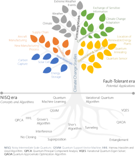
Aaronson S (2015) Read the fine print. Nat Phys 11(4):291–293. https://doi.org/10.1038/nphys3272

Article   CAS   Google Scholar  

Adachi SH, Henderson MP (2015) Application of quantum annealing to training of deep neural networks. https://doi.org/10.48550/arxiv.1510.06356

Ajagekar A, You F (2022) Quantum computing and quantum artificial intelligence for renewable and sustainable energy: a emerging prospect towards climate neutrality. Renew Sustain Energy Rev 165(April):112493. https://doi.org/10.1016/j.rser.2022.112493

Almosni S et al (2018) Material challenges for solar cells in the twenty-first century: directions in emerging technologies. 19(1):336–369. https://doi.org/10.1080/14686996.2018.1433439 . http://www.tandfonline.com/action/journalInformation?show=aimsScope&journalCode=tsta20#.VmBmuzZFCUk

Anul Haq M (2022) CDLSTM: a novel model for climate change forecasting. Comput Mater Continua 71(2):2363–2381. https://doi.org/10.32604/cmc.2022.023059

Article   Google Scholar  

Anul Haq M, Khadar Jilani A, Prabu P (2022) Deep learning based modeling of groundwater storage change. Comput Mater Continua 70(3):4599–4617. https://doi.org/10.32604/cmc.2022.020495

Arrasmith A, Cerezo M, Czarnik P, Cincio L, Coles PJ (2020) Effect of barren plateaus on gradient-free optimization. Quantum. https://doi.org/10.22331/q-2021-10-05-558

Arute F et al (2019) Quantum supremacy using a programmable superconducting processor. Nature 574(7779):505–510. https://doi.org/10.1038/s41586-019-1666-5

Attaallah A, Ahmad Khan R (2022) SMOTEDNN: a novel model for air pollution forecasting and AQI classification. Comput Mater Continua 71(1):1403–1425. https://doi.org/10.32604/cmc.2022.021968

Bauer B, Bravyi S, Motta M, Kin-Lic Chan G (2020) Quantum algorithms for quantum chemistry and quantum materials science. Chem Rev 120(22):12685–12717. https://doi.org/10.1021/ACS.CHEMREV.9B00829/ASSET/IMAGES/MEDIUM/CR9B00829_M030.GIF

Bayerstadler A et al (2021) Industry quantum computing applications. EPJ Quantum Technol. https://doi.org/10.1140/epjqt/s40507-021-00114-x

Berger C et al (2021) Quantum technologies for climate change: preliminary assessment. 1–14

Biamonte J, Wittek P, Pancotti N, Rebentrost P, Wiebe N, Lloyd S (2017a) Quantum machine learning. Nature 549(7671):195–202. https://doi.org/10.1038/nature23474

Biamonte J, Wittek P, Pancotti N, Rebentrost P, Wiebe N, Lloyd S (2017b) Quantum machine learning. Nature 549(7671):195–202. https://doi.org/10.1038/nature23474

Bishop CM (2006) Pattern recognition and machine learning. [Online]. Available: https://link.springer.com/book/9780387310732 . Accessed: 15 Jan 2023

Bittel L, Kliesch M (2021) Training variational quantum algorithms is NP-hard. Phys Rev Lett 127(12):120502. https://doi.org/10.1103/PHYSREVLETT.127.120502/FIGURES/1/MEDIUM

Bobier J-F, Gerbert P, Burchardt J, Gourévitch A (2023) A quantum advantage in fighting climate change | BCG. [Online]. Available: https://www.bcg.com/publications/2020/quantum-advantage-fighting-climate-change . Accessed: Jan. 15, 2023

Bryman A, Bell E (2015) Business research methods, 4th edn. pp 134–156

Cao Y, Romero J, Aspuru-Guzik A (2018) Potential of quantum computing for drug discovery. IBM J Res Dev. https://doi.org/10.1147/JRD.2018.2888987

Cerezo M, Coles PJ (2020) higher order derivatives of quantum neural networks with barren plateaus. Quantum Sci Technol. https://doi.org/10.1088/2058-9565/abf51a

Cerezo M et al (2020) Variational quantum algorithms. Nat Rev Phys 3(9):625–644. https://doi.org/10.1038/s42254-021-00348-9

Cerezo M, Sone A, Volkoff T, Cincio L, Coles PJ (2021) Cost function dependent barren plateaus in shallow parametrized quantum circuits. Nat Commun 12(1):1–12. https://doi.org/10.1038/s41467-021-21728-w

Cerezo M, Verdon G, Huang HY, Cincio L, Coles PJ (2022) Challenges and opportunities in quantum machine learning. Nat Comput Sci 2(9):567–576. https://doi.org/10.1038/s43588-022-00311-3

Chen IC, Hill JK, Ohlemüller R, Roy DB, Thomas CD (2011) Rapid range shifts of species associated with high levels of climate warming. Science (1979) 333(6045):1024–1026. https://doi.org/10.1126/SCIENCE.1206432/SUPPL_FILE/CHEN.SOM.PDF

Childs AM, Kothari R, Somma RD (2015) Quantum algorithm for systems of linear equations with exponentially improved dependence on precision. SIAM J Comput 46(6):1920–1950. https://doi.org/10.1137/16M1087072

Cho A (2019) Google claims quantum computing milestone. Science (1979) 365(6460):1364. https://doi.org/10.1126/SCIENCE.365.6460.1364/ASSET/F0F2FD00-4092-4A46-A30D-270C0DCA460F/ASSETS/GRAPHIC/365_1364_F1.JPEG

Clader BD, Jacobs BC, Sprouse CR (2013) Preconditioned quantum linear system algorithm. Phys Rev Lett 110(25):250504. https://doi.org/10.1103/PhysRevLett.110.250504

Díez-Valle P, Porras D, García-Ripoll JJ (2023) Quantum approximate optimization algorithm pseudo-Boltzmann states. Phys Rev Lett 130(5):050601. https://doi.org/10.1103/PHYSREVLETT.130.050601/FIGURES/5/MEDIUM

Du Y, Hsieh MH, Liu T, Tao D (2020) Expressive power of parametrized quantum circuits. Phys Rev Res 2(3):033125. https://doi.org/10.1103/PHYSREVRESEARCH.2.033125/FIGURES/20/MEDIUM

Espinal L, Morreale BD (2012) Materials challenges in carbon-mitigation technologies. MRS Bull 37(4):431–438. https://doi.org/10.1557/mrs.2012.10

Fan L, Han Z (2022) Hybrid quantum-classical computing for future network optimization. IEEE Netw 36(5):72–76. https://doi.org/10.1109/MNET.001.2200150

Farhi E, Goldstone J, Gutmann S, Sipser M (2000) Quantum computation by adiabatic evolution. http://arxiv.org/abs/quant-ph/0001106 [v1]

Feynman RP (2018) Simulating physics with computers. Feynman Comput. https://doi.org/10.1201/9780429500459-11

Fingerhuth M, Babej T, Wittek P (2018) Open source software in quantum computing. PLoS ONE. https://doi.org/10.1371/journal.pone.0208561

Friedman JR, Patel V, Chen W, Tolpygo SK, Lukens JE (2000) Quantum superposition of distinct macroscopic states. Nature 406(6791):43–46. https://doi.org/10.1038/35017505

Frolov AV (2017) Can a quantum computer be applied for numerical weather prediction? Russ Meteorol Hydrol 42(9):545–553. https://doi.org/10.3103/S1068373917090011/METRICS

Galbraith ED, Eggleston S (2017) A lower limit to atmospheric CO 2 concentrations over the past 800,000 years. Nat Geosci 10(4):295–298. https://doi.org/10.1038/ngeo2914

Giani A, Goff-Eldredge Z (2022) How quantum computing can tackle climate and energy challenges. Eos (washington DC). https://doi.org/10.1029/2022EO220500

Goodfellow I, Bengio Y, Courville A (2016) Deep learning. The MIT Press. [Online]. Available: https://mitpress.mit.edu/9780262035613/deep-learning/ . Accessed: 15 Jan 2023

Google Quantum AI (2023) Cirq. [Online]. Available: https://quantumai.google/cirq . Accessed: 19 Jan 2023

Haidar M, Rančić MJ, Ayral T, Maday Y, Piquemal JP (2023) Open source variational quantum eigensolver extension of the quantum learning machine for quantum chemistry. Wiley Interdiscipl Rev Comput Mol Sci. https://doi.org/10.1002/wcms.1664

Haq MA, Baral P, Yaragal S, Pradhan B (2021) Bulk processing of multi-temporal Modis data, statistical analyses and machine learning algorithms to understand climate variables in the Indian Himalayan Region. Sensors 21(21):7416. https://doi.org/10.3390/s21217416

Haq MA et al (2022) Analysis of environmental factors using AI and ML methods. Sci Rep 12(1):1–16. https://doi.org/10.1038/s41598-022-16665-7

Harrow AW, Montanaro A (2017) Quantum computational supremacy. Nature 549(7671):203–209. https://doi.org/10.1038/nature23458

Harrow AW, Hassidim A, Lloyd S (2009) Quantum algorithm for linear systems of equations. Phys Rev Lett 103(15):150502. https://doi.org/10.1103/PhysRevLett.103.150502

Hastie T, Tibshirani R, Friedman J (2009) The elements of statistical learning. Springer series in statistics. Springer, New York, New York. https://doi.org/10.1007/978-0-387-84858-7

Chapter   Google Scholar  

Havlíček V et al (2019) Supervised learning with quantum-enhanced feature spaces. Nature 567(7747):209–212. https://doi.org/10.1038/s41586-019-0980-2

Huang S, Chang Y, Lin Y, Zhang S (2023) Hybrid quantum–classical convolutional neural networks with privacy quantum computing. Quantum Sci Technol 8(2):025015

IBM (2023) Qiskit. [Online]. Available: https://qiskit.org/ . Accessed: 19 Jan 2023

IPCC (2007) Intergovernmental Panel on climate change 2007: the physical science basis, vol 4, no 4, p 940. Accessed: Jan. 17, 2023. [Online]. Available: http://www.cambridge.org/9780521880091

IPCC (2022) Mitigation of Climate Change Climate Change 2022 Working Group III contribution to the sixth assessment report of the Intergovernmental Panel on Climate Change. [Online]. Available: http://www.ipcc.ch

James G, Witten D, Hastie T, Tibshirani R (2013) An introduction to statistical learning, vol 103. Springer New York, New York. https://doi.org/10.1007/978-1-4614-7138-7

Book   Google Scholar  

Kasliwal K, Jayanthi PN, Jain A, Bahl RK (2023) Enhancing satellite-to-ground communication using quantum key distribution. IET Quantum Commun. https://doi.org/10.1049/qtc2.12053

Kerenidis I, Prakash A (2020) Quantum gradient descent for linear systems and least squares. Phys Rev A 101(2). https://doi.org/10.1103/PhysRevA.101.022316

Kumar A, Augusto de Jesus Pacheco D, Kaushik K, Rodrigues JJPC (2022) Futuristic view of the Internet of quantum drones: review, challenges and research agenda. Veh Commun 36:100487. https://doi.org/10.1016/j.vehcom.2022.100487

Kusumoto T, Mitarai K, Fujii K, Kitagawa M, Negoro M (2019) Experimental quantum kernel machine learning with nuclear spins in a solid. Npj Quantum Inf. https://doi.org/10.1038/s41534-021-00423-0

Lam V (2021) Climate modelling and structural stability. Eur J Philos Sci. https://doi.org/10.1007/s13194-021-00414-0

Landman J et al (2022) Quantum methods for neural networks and application to medical image classification. Quantum. https://doi.org/10.22331/Q-2022-12-22-881

LaRose R (2019) Overview and comparison of gate level quantum software platforms. Quantum. https://doi.org/10.22331/q-2019-03-25-130

Lecun Y, Bengio Y, Hinton G (2015) Deep learning. Nature 521(7553):436–444. https://doi.org/10.1038/nature14539

Li Q, Fang JH, Li W, Liu X (2022) Novel materials and advanced characterization for energy storage and conversion. Energies. https://doi.org/10.3390/en15207536

Li J, Li Y, Steppeler J, Laurian A, Fang F, Knapp D (2023) Challenges and prospects for numerical techniques in atmospheric modeling. Bull Am Meteorol Soc. https://doi.org/10.1175/BAMS-D-22-0269.1

Liu Y, Arunachalam S, Temme K (2021) A rigorous and robust quantum speed-up in supervised machine learning. Nat Phys 17(9):1013–1017. https://doi.org/10.1038/s41567-021-01287-z

Liu HY, Sun TP, Wu YC, Han YJ, Guo GP (2023) Mitigating barren plateaus with transfer-learning-inspired parameter initializations. New J Phys. https://doi.org/10.1088/1367-2630/acb58e

Lloyd S, Mohseni M, Rebentrost P (2013) Quantum algorithms for supervised and unsupervised machine learning. https://doi.org/10.48550/arxiv.1307.0411

Lloyd S, Mohseni M, Rebentrost P (2014) Quantum principal component analysis. Nat Phys 10(9):631–633. https://doi.org/10.1038/nphys3029

Lloyd S, Schuld M, Ijaz A, Izaac J, Killoran N (2020) Quantum embeddings for machine learning. https://doi.org/10.48550/arxiv.2001.03622

Lubasch M, Joo J, Moinier P, Kiffner M, Jaksch D (2019) Variational quantum algorithms for nonlinear problems. Phys Rev A (coll Park). https://doi.org/10.1103/PhysRevA.101.010301

Lüthi D et al (2008) High-resolution carbon dioxide concentration record 650,000–800,000 years before present. Nature 453(7193):379–382. https://doi.org/10.1038/nature06949

Mai H, Le TC, Chen D, Winkler DA, Caruso RA (2022) Machine learning in the development of adsorbents for clean energy application and greenhouse gas capture. Adv Sci. https://doi.org/10.1002/advs.202203899

Mall RK, Bhatt D, Sonkar G, Banerjee T (2014) Simulation modeling and climate change: issues and challenges. In: Environmental science and pollution research international. pp 11605–11608. https://doi.org/10.1007/s11356-014-3096-0

Manski CF, Sanstad AH, DeCanio SJ (2021) Addressing partial identification in climate modeling and policy analysis. Proc Natl Acad Sci USA 118(15):e2022886118. https://doi.org/10.1073/PNAS.2022886118/SUPPL_FILE/PNAS.2022886118.SAPP.PDF

McClean JR, Boixo S, Smelyanskiy VN, Babbush R, Neven H (2018) Barren plateaus in quantum neural network training landscapes. Nat Commun 9(1):1–6. https://doi.org/10.1038/s41467-018-07090-4

Meinshausen M et al (2017) Historical greenhouse gas concentrations for climate modelling (CMIP6). Geosci Model Dev 10(5):2057–2116. https://doi.org/10.5194/GMD-10-2057-2017

Melillo J, Richmond T G. Y.-T. national climate, and undefined (2014) Climate change impacts in the United States. globalchange.gov. Accessed: Jan. 17, 2023. [Online]. Available: https://www.globalchange.gov/sites/globalchange/files/Ch_0a_FrontMatter_ThirdNCA_GovtReviewDraft_Nov_22_2013_clean.pdf

Mondal D, Halder D, Halder S, Maitra R (2023) Development of a compact Ansatz via operator commutativity screening: digital quantum simulation of molecular systems. J Chem Phys. https://doi.org/10.1063/5.0153182

Montanaro A (2016) Quantum algorithms: an overview. Npj Quantum Inf 2(1):1–8. https://doi.org/10.1038/npjqi.2015.23

Murphy KP (2012) Machine learning. The MIT Press. [Online]. Available: https://mitpress.mit.edu/9780262018029/machine-learning/ . Accessed: 15 Jan 2023

Orús R, Mugel S, Lizaso E (2019) Quantum computing for finance: overview and prospects. Rev Phys 4:100028. https://doi.org/10.1016/J.REVIP.2019.100028

Otgonbaatar S et al (2023) Quantum computing for climate change detection, climate modeling, and climate digital twin. TechRxiv. https://doi.org/10.36227/techrxiv.24478663.v1

Pirandola S, Bardhan BR, Gehring T, Weedbrook C, Lloyd S (2018) Advances in photonic quantum sensing. Nat Photonics 12(12):724–733. https://doi.org/10.1038/s41566-018-0301-6

Preskill J (2018) Quantum computing in the NISQ era and beyond. Quantum. https://doi.org/10.22331/q-2018-08-06-79

PyTorch. [Online]. Available: https://pytorch.org/ . Accessed: 22 Mar 2023

Q# and the Quantum Development Kit | Microsoft Azure. [Online]. Available: https://azure.microsoft.com/en-us/resources/development-kit/quantum-computing/#overview . Accessed: 22 Mar 2023

Quantum Cloud Service-Quantum Computing Service-Amazon Braket-AWS. [Online]. Available: https://aws.amazon.com/braket/ . Accessed: 22 Mar 2023

Rebentrost P, Mohseni M, Lloyd S (2014) Quantum support vector machine for big data classification. Phys Rev Lett 113(13):130503. https://doi.org/10.1103/PhysRevLett.113.130503

Rice JE et al (2021) Quantum computation of dominant products in lithium–sulfur batteries. J Chem Phys 154(13):134115. https://doi.org/10.1063/5.0044068

Riexinger F, Kutas M, Haase B, Bortz M, von Freymann G (2023) General simulation method for quantum-sensing systems. Laser Photon Rev. https://doi.org/10.1002/lpor.202200945

Rigetti Computing (2023) Forest SDK. [Online]. Available: https://www.rigetti.com/what-we-build . Accessed: 19 Jan 2023

Romero J, Aspuru-Guzik A (2019) Variational quantum generators: generative adversarial quantum machine learning for continuous distributions. Adv Quantum Technol. https://doi.org/10.48550/arxiv.1901.00848

Romero J, Olson JP, Aspuru-Guzik A (2017) Quantum autoencoders for efficient compression of quantum data. Quantum Sci Technol 2(4):045001. https://doi.org/10.1088/2058-9565/AA8072

Sack SH, Medina RA, Kueng R, Serbyn M (2023) Recursive greedy initialization of the quantum approximate optimization algorithm with guaranteed improvement. Phys Rev A (coll Park). https://doi.org/10.1103/PhysRevA.107.062404

Safari A, Ghavifekr AA (2021) Quantum neural networks (QNN) application in weather prediction of smart grids. In: 2021 11th smart grid conference, SGC 2021. https://doi.org/10.1109/SGC54087.2021.9664117

Sakhnenko A, O’Meara C, Ghosh KJB, Mendl CB, Cortiana G, Bernabé-Moreno J (2021) Hybrid classical-quantum autoencoder for anomaly detection. Quantum Mach Intell. https://doi.org/10.1007/s42484-022-00075-z

Salart D, Baas A, Branciard C, Gisin N, Zbinden H (2008) Testing the speed of ‘spooky action at a distance.’ Nature 454(7206):861–864. https://doi.org/10.1038/nature07121

Scherer A, Valiron B, Mau S-C, Alexander S, van den Berg E, Chapuran TE (2015) Concrete resource analysis of the quantum linear system algorithm used to compute the electromagnetic scattering cross section of a 2D target. Quantum Inf Process. https://doi.org/10.1007/s11128-016-1495-5

Schuld M, Killoran N (2019) Quantum machine learning in feature Hilbert spaces. Phys Rev Lett 122(4):040504. https://doi.org/10.1103/PHYSREVLETT.122.040504/FIGURES/5/MEDIUM

Schuld M, Sinayskiy I, Petruccione F (2014) The quest for a quantum neural network. Quantum Inf Process 13(11):2567–2586. https://doi.org/10.1007/s11128-014-0809-8

Schuld M, Sinayskiy I, Petruccione F (2015) An introduction to quantum machine learning. Contemp Phys 56(2):172–185. https://doi.org/10.1080/00107514.2014.964942

Schuld M, Bocharov A, Svore KM, Wiebe N (2020) Circuit-centric quantum classifiers. Phys Rev A (coll Park) 101(3):032308. https://doi.org/10.1103/PHYSREVA.101.032308/FIGURES/4/MEDIUM

Sherbert K, Jayaraj A, Buongiorno Nardelli M (2022) Quantum algorithm for electronic band structures with local tight-binding orbitals. Sci Rep. https://doi.org/10.1038/s41598-022-13627-x

Skolik A, McClean JR, Mohseni M, van der Smagt P, Leib M (2020) Layerwise learning for quantum neural networks. Quantum Mach Intell. https://doi.org/10.1007/s42484-020-00036-4

Stocker TF et al (2014) Climate Change 2013—the physical science basis: Working Group I contribution to the fifth assessment report of the Intergovernmental Panel on Climate Change, vol 9781107057999, pp 1–1535. https://doi.org/10.1017/CBO9781107415324 .

Sun K et al (2023) Quantum simulation of polarized light-induced electron transfer with a trapped-ion Qutrit system. J Phys Chem Lett 14(26):6071–6077. https://doi.org/10.1021/acs.jpclett.3c01166

Sutton RS, Barto AG (2018) Reinforcement learning. The MIT Press. [Online]. Available: https://mitpress.mit.edu/9780262039246/reinforcement-learning/ . Accessed: 15 Jan 2023

Tennie F, Palmer TN (2023) Quantum computers for weather and climate prediction: the good, the bad, and the noisy. Bull Am Meteorol Soc 104(2):E488–E500. https://doi.org/10.1175/BAMS-D-22-0031.1

Uvarov AV, Biamonte JD (2021) On barren plateaus and cost function locality in variational quantum algorithms. J Phys A Math Theor 54(24):245–301

Vapnik VN (2000) The nature of statistical learning theory. Nat Stat Learn Theory. https://doi.org/10.1007/978-1-4757-3264-1

Variational Quantum Classifier | Quantum Machine Learning (with IBM). [Online]. Available: https://open.hpi.de/courses/qc-machineLearning2023/items/18fQtYG69QeCqwg73bPIEZ . Accessed: 01 June 2023

Verdon G, Pye J, Broughton M (2018) A universal training algorithm for quantum deep learning. https://doi.org/10.48550/arxiv.1806.09729

Verdon G, Broughton M., McClean JR, Sung KJ, Babbush R, Jiang Z, Neven H, Mohseni M (2019) Learning to learn with quantum neural networks via classical neural networks. https://doi.org/10.48550/arxiv.1907.05415

Vijayavenkataraman S, Iniyan S, Goic R (2012) A review of climate change, mitigation and adaptation. Renew Sustain Energy Rev 16(1):878–897. https://doi.org/10.1016/j.rser.2011.09.009

Volkoff T, Coles PJ (2021) Large gradients via correlation in random parameterized quantum circuits. Quantum Sci Technol 6(2):025008. https://doi.org/10.1088/2058-9565/ABD891

von Lilienfeld OA (2018) Quantum machine learning in chemical compound space. Angew Chem Int Ed 57(16):4164–4169. https://doi.org/10.1002/ANIE.201709686

Wan KH, Dahlsten O, Kristjánsson H, Gardner R, Kim MS (2017) Quantum generalisation of feedforward neural networks. Npj Quantum Inf 3(1):1–8. https://doi.org/10.1038/s41534-017-0032-4

What To Look For In A Quantum Machine Learning Framework | by Frank Zickert | Quantum Machine Learning | Towards Data Science (2023) Zickert Frank. [Online]. Available: https://towardsdatascience.com/what-to-look-for-in-a-quantum-machine-learning-framework-b7a7c281aa4f . Accessed: 21 Mar 2023

Wiebe N, Braun D, Lloyd S (2012) Quantum algorithm for data fitting. Phys Rev Lett 109(5):050505. https://doi.org/10.1103/PhysRevLett.109.050505

Wossnig L, Zhao Z, Prakash A (2018) Quantum linear system algorithm for dense matrices. Phys Rev Lett 120(5):050502. https://doi.org/10.1103/PhysRevLett.120.050502

Xanadu (2023) PennyLane. [Online]. Available: https://pennylane.ai/ . Accessed: 19 Jan 2023

Xu Y-Z, Huang Y, Ye Z, Li L (2018) A note on ‘Quantum Algorithm for Linear Systems of Equations’. [Online]. Available: http://arxiv.org/abs/1802.07194 [v1]

Yamamoto M et al (2022) Increased interglacial atmospheric CO 2 levels followed the mid-Pleistocene transition. Nat Geosci 15(4):307–313. https://doi.org/10.1038/s41561-022-00918-1

Yarkoni S, Raponi E, Bäck T, Schmitt S (2022) Quantum annealing for industry applications: introduction and review. http://arxiv.org/abs/2112.07491v3 . https://doi.org/10.1088/1361-6633/ac8c54

Yoshioka N, Sato T, Nakagawa YO, Ohnishi YY, Mizukami W (2022) Variational quantum simulation for periodic materials. Phys Rev Res. https://doi.org/10.1103/PhysRevResearch.4.013052

Yuan X, Endo S, Zhao Q, Li Y, Benjamin SC (2019) Theory of variational quantum simulation. Quantum 3:191. https://doi.org/10.22331/q-2019-10-07-191

Zhao D et al (2021) Characterizing quantum simulations with quantum tomography on a spin quantum simulator. Phys Rev A (coll Park) 103(5):052403. https://doi.org/10.1103/PHYSREVA.103.052403/FIGURES/3/MEDIUM

Zhao M, Kim D, Lee YH, Yang H, Cho S (2023) Quantum sensing of thermoelectric power in low-dimensional materials. Adv Mater. https://doi.org/10.1002/ADMA.202106871

Zubov D, Volponi F, Khosravy M (2015) D-wave quantum computing Ising model: a case study for the forecasting of heat waves. In: ICCAIS 2015—4th international conference on control, automation and information sciences, pp 149–152. https://doi.org/10.1109/ICCAIS.2015.7338651

Download references

Acknowledgements

The authors would like to gratefully acknowledge the support of King Fahd University of Petroleum & Minerals (KFUPM) in conducting this research.

The authors have not disclosed any funding.

Author information

Authors and affiliations.

Applied Research Center for Environment and Marine Studies, King Fahd Univeristy of Petroleum and Minerals (KFUPM), 31261, Dhahran, Saudi Arabia

Syed Masiur Rahman, Omar Hamad Alkhalaf, Md Shafiul Alam, Surya Prakash Tiwari & Sarah Mohammed Al-Judaibi

Integrated Research Center for Renewable Energy and Power Systems, King Fahd Univeristy of Petroleum and Minerals (KFUPM), 31261, Dhahran, Saudi Arabia

Md Shafiullah

Department of Electrical Engineering, King Fahd Univeristy of Petroleum and Minerals (KFUPM), 31261, Dhahran, Saudi Arabia

Fahad Saleh Al-Ismail

You can also search for this author in PubMed   Google Scholar

Corresponding author

Correspondence to Syed Masiur Rahman .

Ethics declarations

Conflict of interest.

The authors have not disclosed any competing interests.

Rights and permissions

Springer Nature or its licensor (e.g. a society or other partner) holds exclusive rights to this article under a publishing agreement with the author(s) or other rightsholder(s); author self-archiving of the accepted manuscript version of this article is solely governed by the terms of such publishing agreement and applicable law.

Reprints and permissions

About this article

Rahman, S.M., Alkhalaf, O.H., Alam, M.S. et al. Climate Change Through Quantum Lens: Computing and Machine Learning. Earth Syst Environ (2024). https://doi.org/10.1007/s41748-024-00411-2

Download citation

Received : 07 January 2024

Revised : 16 April 2024

Accepted : 23 May 2024

Published : 04 June 2024

DOI : https://doi.org/10.1007/s41748-024-00411-2

Share this article

Anyone you share the following link with will be able to read this content:

Sorry, a shareable link is not currently available for this article.

Provided by the Springer Nature SharedIt content-sharing initiative

• Quantum computing
• Machine learning
• Quantum machine learning
• Climate change studies
• Noisy intermediate scale quantum era
• Fault-tolerant quantum era
• Find a journal
• Publish with us
• Track your research