integer programming excel solver examples

How to Solve Integer Linear Programming in Excel (With Easy Steps)

In this article, we will learn to solve integer linear programming in Excel. In Microsoft Excel, users can quickly determine the solution of an integer linear program using the Solver add-in . Today, we will demonstrate this process with easy and quick steps. We will also discuss an example of a mixed-integer linear programming problem in the last section of this article. So, without any delay, let’s start the discussion.

What Is Integer Linear Programming?

Integer linear programming is a type of mathematical method that consists of integer variables and linear objective functions and equations. With the help of linear programming, we can determine the minimum or maximum outcome of a given problem with some conditions. It is a tool that can be used to achieve a way to apply the limited resources in the best possible manner. All types of linear programming include some main factors. They are given below:

Decision Variables: We determine the decision variables that minimize or maximize the objective function.
Objective Function: This is a function that helps us to determine the decision variables. It expresses the relation between the result and the variables.
Constraints: Constraints are also functions that denote different conditions on possible solutions.

Besides integer linear programming, we will also see an example of mixed-integer linear programming. The mixed-integer linear programming has both continuous and integer variables.

Solve Integer Linear Programming in Excel: Step-by-Step Procedures

To explain the step-by-step procedures, we will use the question below. You need to read it carefully to understand the basic things. You must derive the Constraints and Objective function after reading the question carefully.

Suppose, a machine is used to produce two interchangeable products. The daily capacity of the machine can produce at most 20 units of product 1 and 10 units of product 2 . Alternatively, the machine can be adjusted to produce at most 12 units of product 1 and 25 units of product 2 daily. Market analysis shows that the maximum daily demand for the two products combined is 35 units. Given that the unit profits for the two respective products are $10 and $12 , which of the two machine settings should be selected?

STEP 1: Analyze Question and Create Dataset

First of all, we need to understand the given integer linear programming problem and analyze it carefully.
Analyzing the above question, we have the findings below.

Decision Variables:

X1: Production quantity of product 1 .
X2: Production quantity of product 2 .
Y: 1 if the first setting is selected or 0 if the second setting is selected.

Objective Function:

Here, the objective function is:

Z=10X1+12X2

Constraints:

We can mainly find 3 constraints from the above question. They are:

X1+X2<=35

Because the market analysis shows that the maximum daily demand for the two products combined is 35 units.

X1-8Y<=12

This constraint is specific for product 1 .

X2+15Y<=25

It is the constraint for the second product.

The value of Y will be 0 or 1 .

X1,X2>=0

The quantity of the products can not be negative.

In the following step, we have created a dataset like the picture below keeping the constraints, functions, and variables in mind. You can change it according to your needs.

Step-by-Step Procedures to Solve Integer Linear Programming in Excel

Read More: How to Do Linear Programming in Excel

STEP 2: Load Solver Add-in in Excel

Secondly, we need to load the Solver add-in in Excel. If it is already loaded in your Excel, then, you can move forward to step 3 .
To do so, click on the File tab.

After that, select Options from the left – bottom corner of the screen.
It will open the Excel Options window.

In the Excel Options window, select Add-ins .
Then, select Excel Add-ins and click on Go in the Manage box.
An Add-ins message box will pop up.

Check Solver Add-in and select OK from the message box.

Finally, you will see the Solver feature in the Analysis section of the Data tab.

Read More: How to Solve Blending Linear Programming Problem with Excel Solver

STEP 3: Fill Coefficients of Constraints and Objective Function

Thirdly, you need to fill the constraints and objective function in the dataset.
Here, we will mainly insert the coefficients of the constraints and objective function.
Our first Constraint is that X1+X2<=35 . It means if the first setting is selected then, the sum of the products should be equal to or less than 35 .
So, the coefficient of X1 is 1 and X2 is 2 .
Also, the equation indicates the first setting, so the coefficient of Y is 1 .
The sign is <= .
And the limit is 35 .

Repeat the previous instruction and fill in the coefficients of all the constraints.

After that, select Cell E10 and type the formula:

In this formula, we have used the SUMPRODUCT function to calculate the product of decision variables with the respected constraints variables and then add them up. In this case, Cell B6 will be multiplied by Cell B10 , Cell C6 by Cell C10 , and Cell D6 by Cell D10 . Then, all the products will be added together.

Hit Enter and drag the Fill Handle down.

Now, fill the coefficients of the objective function in Cell B16 to C16 .
In our case, the objective function is Z = 10X1+12X2 .

Again, select Cell E16 and type the formula below:

In the end, press Enter and you will see a dataset like the one below after inserting the coefficients and formulas.

STEP 4: Insert Solver Parameters

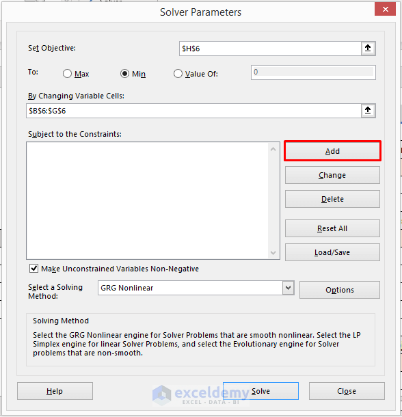
In step 4, go to the Data tab and select Solver from the Analyze section. It will open the Solver Parameters window.

In the Set Objective box, you need to type the cell that will contain the value of the objective function .
So, we have typed $E$16 here.
Here, we are trying to find the maximum result.
So, we have selected Max for the next step.
In the ‘ By Changing Variable Cells ’ type $B$6:$D$6 . It contains the decision variables.

STEP 5: Add Subject to Constraints

In the fifth step, we need to add subjects to the constraints.
We need to denote the type of variables whether they are binary or integer and the relation of the constraints.
For that purpose, click on Add . It will open the Add Constraint dialog box.

In the Add Constraint window, type $D$6 in the Cell Reference box and select bin from the drop-down menu.
Cell D6 holds the value of Y which is 0 or 1 . That indicates binary numbers. That is why we have selected the bin here.
Click OK to proceed.

Again, click on Add .

This time, type $E$10:$E$12 in the Cell Reference box, <= symbol from the drop-down menu, and =$G$10:$G$12 in the Constraint box.
Then, click OK .

Once again, click Add in the Solver Parameters window.

Now, type $B$6:$C$6 in the Cell Reference box and select int from the drop-down menu.
Cell B6 and C6 store the values of X1 and X2 which are integers.
Again, click OK .

STEP 6: Select Solving Method

In step 6, select Simplex LP in the ‘ Select a Solving Method ’ section and click on Solve .
Make sure ‘ Make Unconstrained Variables Non-Negative ’ is checked.

After clicking on Solve , the Solver Results window will appear.
Select OK from there.

STEP 7: Solution of Integer Linear Programming

Finally, you will find the solutions in your desired cells on the excel sheet.
In this case, the second machine setting will provide us with the best output.

STEP 8: Generate Answer Report

Additionally, you can generate the answer report.
In order to do that, select Answer in the Reports section of the Solver Results window and click OK .

Lastly, you will find the report on a new sheet.

Mixed Integer Linear Programming Example in Excel

In this section, we will discuss a simple example of mixed-integer linear programming in Excel. You can follow the quick steps to solve mixed-integer linear programming in Excel easily. Let’s take a look at the objective function and constraints for this example.

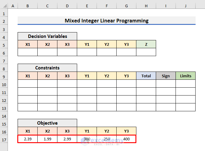
Z=2.39X1+1.99X2+2.99X3+300Y1+250Y2+400Y3

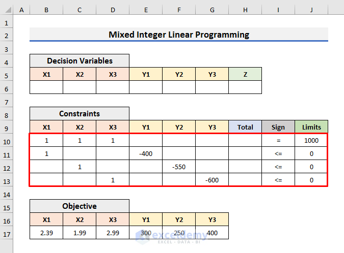
X1+X2+X3=1000
X1-400Y1<=0
X2-550Y2<=0
X3-600Y3<=0

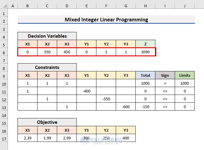
Here, X1 , X2 , and X3 are integers. On the other hand, Y1 , Y2 , and Y3 are binary numbers. Also, we need to find the minimum value of Z .

Let’s follow the steps below to learn everything about the example.

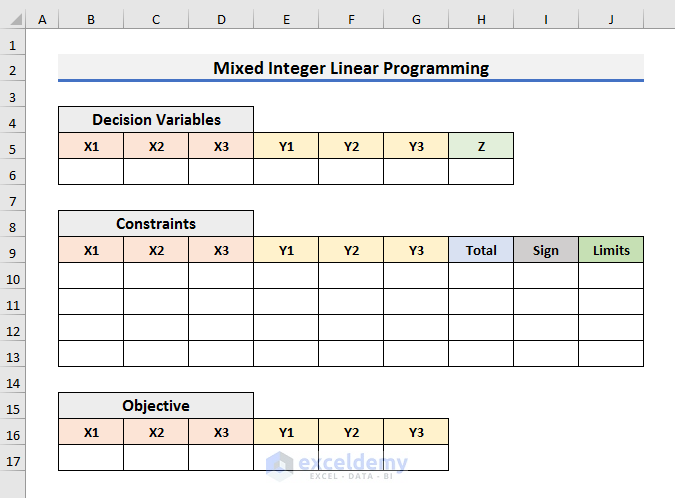
Firstly, create a dataset to store the coefficients of Decision Variables , Constraints , and Objective Function .

integer programming excel solver examples

Secondly, type mixed coefficients of the variables of the Objective Function .

Thirdly, type the coefficients of the variables of Constraints like the picture below. Keep the Total column empty.

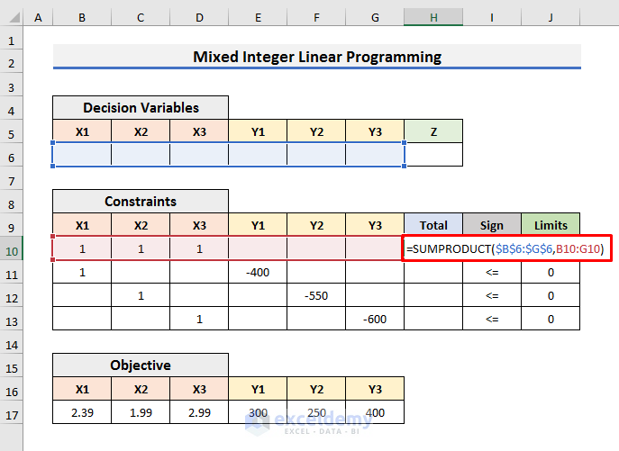
After that, select Cell H10 and type the formula below:

Press Enter and drag the Fill Handle down.

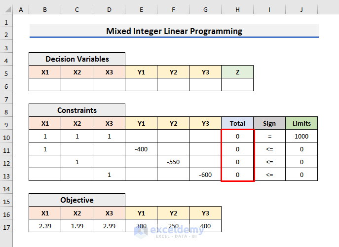
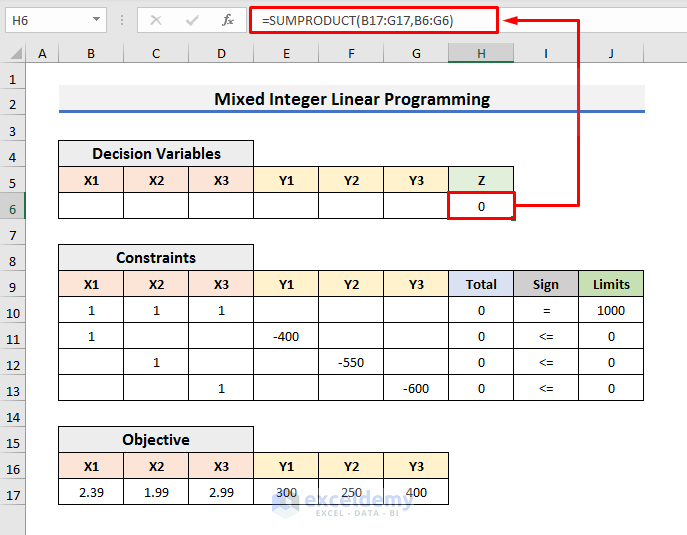
Now, type the formula below in Cell H6 :
Hit Enter .

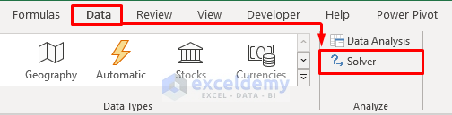
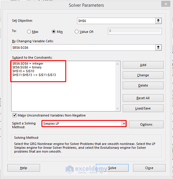
In the following step, go to the Data tab and select Solver . It will open the Solver Parameters window.

In the Solver Parameters window, set the objective at Cell $H$6 to Min by changing variable cells $B$6:$G$6 .

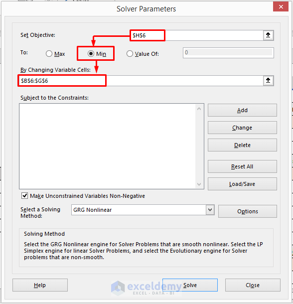
Then, click on Add .

At this moment, add the Constraints one by one and choose Simplex LP as the Solving Method .
Click on Solve to proceed.

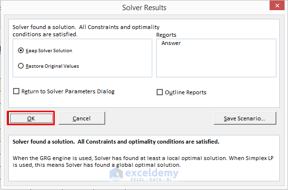
As a result, the Solver Results window will appear.
Click OK from there.

Finally, the results will look like the picture below.

Read More: How to Perform Mixed Integer Linear Programming in Excel

Download Practice Book

You can download the practice book from here.

In this article, we have demonstrated step-by-step procedures to Solve Integer Linear Programming in Excel. I hope this article will help you to perform your tasks easily. Moreover, we have also added the practice book at the beginning of the article. Furthermore, you can download it to test your skills. Last of all, if you have any suggestions or queries, feel free to ask in the comment section below.

How to Calculate Shadow Price Linear Programming in Excel
Graph Linear Programming in Excel
How to Find Optimal Solution with Linear Programming in Excel
How to Solve Transportation Problem with Linear Programming
How to Do Linear Programming with Sensitivity Analysis in Excel

<< Go Back to Excel Linear Programming | Solver in Excel | Learn Excel

What is ExcelDemy?

Tags: Excel Linear Programming

Mursalin Ibne Salehin holds a BSc in Electrical and Electronics Engineering from Bangladesh University of Engineering and Technology. Over the past 2 years, he has actively contributed to the ExcelDemy project, where he authored over 150 articles. He has also led a team with content development works. Currently, he is working as a Reviewer in the ExcelDemy Project. He likes using and learning about Microsoft Office, especially Excel. He is interested in data analysis with Excel, machine learning,... Read Full Bio

Hi Mursalin. Could you please explain how you got the constraint equations?

Hi KIM, Thanks for your comment. To explain the step-by-step solution, we used the following question here.

“Suppose, a machine is used to produce two interchangeable products. The daily capacity of the machine can produce at most 20 units of product 1 and 10 units of product 2 . Alternatively, the machine can be adjusted to produce at most 12 units of product 1 and 25 units of product 2 daily. Market analysis shows that the maximum daily demand for the two products combined is 35 units. Given that the unit profits for the two respective products are $10 and $12 , which of the two machine settings should be selected?”

This question is also stated before starting STEP 1 .

Analyzing the above question, we can find the following constraints:

Constraint 1: X1+X2 Because the maximum daily demand for the two products combined is 35 units. Here, X1 is the quantity of Product 1 and X2 is the quantity of Product 2.

Constraint 2: X1-8Y This constraint is for Product 1. In this constraint, we have combined the conditions for both settings for Product 1. In setting 1, product 1 can be produced at most 20 units; in setting 2, product 2 can be produced at most 12 units. Here, Y denotes which setting is selected. If setting 1 is selected, then Y will be 1 and if setting 2 is selected, then Y will be 0. For example, if setting 1 is selected, then we can set Y=1. So, the equation will be: X1-8.1 As a result, the simplified constraint will be X1 which clearly states the condition for product 1 stated in the first setting.

Constraint 3: X2+15Y This constraint is for Product 2. In this constraint, we have combined the conditions for both settings for Product 2. In setting 1, product 2 can be produced at most 10 units; in setting 2, product 2 can be produced at most 25 units. Here, Y denotes which setting is selected. If setting 1 is selected, then Y will be 1 and if setting 2 is selected, then Y will be 0. For example, if setting 1 is selected, then we can set Y=1. So, the equation will be: X2+15.1 As a result, the simplified constraint will be X2 which clearly states the condition for product 2 stated in the first setting.

Constraint 4: Y={0,1} The value of Y will be 0 or 1. 1 represents the selection of setting 1 and 0 represents the selection of setting 2.

Non–Negative restriction: X1,X2>=0 The quantity of the products can not be negative.

Constraints 1, 2 & 3 are the main constraints here.

In the Mixed Integer Linear Programming part, we have used a set of conditions as constraints where X1 , X2 , and X3 are integers and Y1 , Y2 , and Y3 are binary numbers. I hope this explanation of the constraints will help you. Please let me know if you have any queries.

Regards Mursalin, Exceldemy.

How to use Solver in Excel with examples

The tutorial explains how to add and where to find Solver in different Excel versions, from 2016 to 2003. Step-by-step examples show how to use Excel Solver to find optimal solutions for linear programming and other kinds of problems.

Everyone knows that Microsoft Excel contains a lot of useful functions and powerful tools that can save you hours of calculations. But did you know that it also has a tool that can help you find optimal solutions for decision problems?

In this tutorial, we are going to cover all essential aspects of the Excel Solver add-in and provide a step-by-step guide on how to use it most effectively.

What is Excel Solver?

Excel Solver belongs to a special set of commands often referred to as What-if Analysis Tools. It is primarily purposed for simulation and optimization of various business and engineering models.

The Excel Solver add-in is especially useful for solving linear programming problems, aka linear optimization problems, and therefore is sometimes called a linear programming solver . Apart from that, it can handle smooth nonlinear and non-smooth problems. Please see Excel Solver algorithms for more details.

How to add Solver to Excel

The Solver add-in is included with all versions of Microsoft Excel beginning with 2003, but it is not enabled by default.

To add Solver to your Excel, perform the following steps:

In Excel 2010 - Excel 365, click File > Options . In Excel 2007, click the Microsoft Office button, and then click Excel Options .

Open the Excel Options dialog to get to the Excel Add-ins list.

To get Solver on Excel 2003 , go to the Tools menu, and click Add-Ins . In the Add-Ins available list, check the Solver Add-in box, and click OK .

Where is Solver in Excel?

Where is Solver in Excel 2003?

Now that you know where to find Solver in Excel, open a new worksheet and let's get started!

How to use Solver in Excel

Before running the Excel Solver add-in, formulate the model you want to solve in a worksheet. In this example, let's find a solution for the following simple optimization problem.

Problem . Supposing, you are the owner of a beauty salon and you are planning on providing a new service to your clients. For this, you need to buy a new equipment that costs $40,000, which should be paid by instalments within 12 months.

Goal : Calculate the minimal cost per service that will let you pay for the new equipment within the specified timeframe.

And now, let's see how Excel Solver can find a solution for this problem.

1. Run Excel Solver

2. define the problem.

The Solver Parameters window will open where you have to set up the 3 primary components:

Objective cell

Variable cells

Constraints.

Exactly what does Excel Solver do with the above parameters? It finds the optimal value (maximum, minimum or specified) for the formula in the Objective cell by changing the values in the Variable cells, and subject to limitations in the Constraints cells.

The Objective cell ( Target cell in earlier Excel versions) is the cell containing a formula that represents the objective, or goal, of the problem. The objective can be to maximize, minimize, or achieve some target value.

Variable cells ( Changing cells or Adjustable cells in earlier versions) are cells that contain variable data that can be changed to achieve the objective. Excel Solver allows specifying up to 200 variable cells.

In this example, we have a couple of cells whose values can be changed:

Projected clients per month (B4) that should be less than or equal to 50; and
Cost per service (B5) that we want Excel Solver to calculate.

The Excel Solver Constrains are restrictions or limits of the possible solutions to the problem. To put it differently, constraints are the conditions that must be met.

To add a constraint(s), do the following:

Click the Add button right to the " Subject to the Constraints " box.

In the Constraint window, enter a constraint.
Click the Add button to add the constraint to the list.

Click the Add button to add the constraint to the list.

Continue entering other constraints.
After you have entered the final constraint, click OK to return to the main Solver Parameters window.

Excel Solver allows specifying the following relationships between the referenced cell and the constraint.

Less than or equal to , equal to , and greater than or equal to . You set these relationships by selecting a cell in the Cell Reference box, choosing one of the following signs: <= , =, or >= , and then typing a number, cell reference / cell name, or formula in the Constraint box (please see the above screenshot).
Integer . If the referenced cell must be an integer, select int , and the word integer will appear in the Constraint box.
Different values . If each cell in the referenced range must contain a different value, select dif , and the word AllDifferent will appear in the Constraint box.
Binary . If you want to limit a referenced cell either to 0 or 1, select bin , and the word binary will appear in the Constraint box.

To edit or delete an existing constraint do the following:

In the Solver Parameters dialog box, click the constraint.
To modify the selected constraint, click Change and make the changes you want.
To delete the constraint, click the Delete button.

In this example, the constraints are:

B3=40000 - cost of the new equipment is $40,000.
B4<=50 - the number of projected patients per month in under 50.

3. Solve the problem

After you've configured all the parameters, click the Solve button at the bottom of the Solver Parameters window (see the screenshot above) and let the Excel Solver add-in find the optimal solution for your problem.

Depending on the model complexity, computer memory and processor speed, it may take a few seconds, a few minutes, or even a few hours.

The Solver Result window will close and the solution will appear on the worksheet right away.

If the Excel Solver has been processing a certain problem for too long, you can interrupt the process by pressing the Esc key. Excel will recalculate the worksheet with the last values found for the Variable cells.
To get more details about the solved problem, click a report type in the Reports box, and then click OK . The report will be created on a new worksheet:

Excel Solver examples

Below you will find two more examples of using the Excel Solver addin. First, we will find a solution for a well-known puzzle, and then solve a real-life linear programming problem.

Excel Solver example 1 (magic square)

I believe everyone is familiar with "magic square" puzzles where you have to put a set of numbers in a square so that all rows, columns and diagonals add up to a certain number.

For instance, do you know a solution for the 3x3 square containing numbers from 1 to 9 where each row, column and diagonal adds up to 15?

It's probably no big deal to solve this puzzle by trial and error, but I bet the Solver will find the solution faster. Our part of the job is to properly define the problem.

With all the formulas in place, run Solver and set up the following parameters:

Set Objective . In this example, we don't need to set any objective, so leave this box empty.
Variable Cells . We want to populate numbers in cells B2 to D4, so select the range B2:D4.
$B$2:$D$4 = AllDifferent - all of the Variable cells should contain different values.
$B$2:$D$4 = integer - all of the Variable cells should be integers.
$B$5:$D$5 = 15 - the sum of values in each column should equal 15.
$E$2:$E$4 = 15 - the sum of values in each row should equal 15.
$B$7:$B$8 = 15 - the sum of both diagonals should equal 15.

Excel Solver example 2 (linear programming problem)

This is an example of a simple transportation optimization problem with a linear objective. More complex optimization models of this kind are used by many companies to save thousands of dollars each year.

Problem : You want to minimize the cost of shipping goods from 2 different warehouses to 4 different customers. Each warehouse has a limited supply and each customer has a certain demand.

Goal : Minimize the total shipping cost, not exceeding the quantity available at each warehouse, and meeting the demand of each customer.

Source data

Formulating the model

To define our linear programming problem for the Excel Solver, let's answer the 3 main questions:

What decisions are to be made? We want to calculate the optimal quantity of goods to deliver to each customer from each warehouse. These are Variable cells (B7:E8).
What are the constraints? The supplies available at each warehouse (I7:I8) cannot be exceeded, and the quantity ordered by each customer (B10:E10) should be delivered. These are Constrained cells .
What is the goal? The minimal total cost of shipping. And this is our Objective cell (C12).

Formulating the model using Excel formulas

To make our transportation optimization model easier to understand, create the following named ranges:

The last thing left for you to do is configure the Excel Solver parameters:

Objective: Shipping_cost set to Min
Variable cells: Products_shipped
Constraints: Total_received = Ordered and Total_shipped <= Available

How to save and load Excel Solver scenarios

When solving a certain model, you may want to save your Variable cell values as a scenario that you can view or re-use later.

For example, when calculating the minimal service cost in the very first example discussed in this tutorial, you may want to try different numbers of projected clients per month and see how that affects the service cost. At that, you may want to save the most probable scenario you've already calculated and restore it at any moment.

Saving an Excel Solver scenario boils down to selecting a range of cells to save the data in. Loading a Solver model is just a matter of providing Excel with the range of cells where your model is saved. The detailed steps follow below.

Saving the model

To save the Excel Solver scenario, perform the following steps:

Open the worksheet with the calculated model and run the Excel Solver.

Excel will save your current model, which may look something similar to this:

The current Excel Solver scenario is saved.

Loading the saved model

When you decide to restore the saved scenario, do the following:

In the Solver Parameters window, click the Load/Save button.

Select the range of cells containing the saved model and click Load.

This will open the main Excel Solver window with the parameters of the previously saved model. All you need to do is to click the Solve button to re-calculate it.

Excel Solver algorithms

When defining a problem for the Excel Solver, you can choose one of the following methods in the Select a Solving Method dropdown box:

GRG Nonlinear. Generalized Reduced Gradient Nonlinear algorithm is used for problems that are smooth nonlinear, i.e. in which at least one of the constraints is a smooth nonlinear function of the decision variables. More details can be found here .
LP Simplex . The Simplex LP Solving method is based the Simplex algorithm created by an American mathematical scientist George Dantzig. It is used for solving so called Linear Programming problems - mathematical models whose requirements are characterized by linear relationships, i.e. consist of a single objective represented by a linear equation that must be maximized or minimized. For more information, please check out this page .
Evolutionary . It is used for non-smooth problems, which are the most difficult type of optimization problems to solve because some of the functions are non-smooth or even discontinuous, and therefore it's difficult to determine the direction in which a function is increasing or decreasing. For more information, please see this page .

This is how you can use Solver in Excel to find the best solutions for your decision problems. At the end of this post, you can download the sample workbook with all the examples discussed in this tutorial and reverse-engineer them for better understanding. I thank you for reading and hope to see you on our blog next week.

Practice workbook for download

Optimization Modeling with Solver in Excel

May 18, 2015 By Stephen L. Nelson Leave a Comment

Excel’s Solver tool lets you solve optimization-modeling problems, also commonly known as linear programming programs. With an optimization-modeling problem, you want to optimize an objective function but at the same time recognize that there are constraints, or limits. While this abstract definition sounds complicated, at least at the conceptual level, optimization modeling makes common sense once you provide a concrete example.

EasyRefresher: How Optimization Modeling Works

Suppose, for example, that you’re a residential real estate developer and contractor. You create and sell two products: building lots and houses. Suppose that you make $20,000 on each home you build and $15,000 on each building lot you develop and then sell. Your princi- pal financial objective is to maximize your profits, and this objective can be expressed as an objective function, or equation, that you want to maximize:

$15,000*Lots+$20,000*Houses=Profits

Of course, any objective function is limited by certain constraints. To continue with the fictional case of residential development, suppose that you have two principal limiting fac- tors: working capital and bulldozer capacity. Your working capital of $1,200,000 limits the number of lots and houses you can annually sell because every lot requires a $50,000 cash investment and every house requires a $25,000 cash investment. The fact that you have a single bulldozer available for only 3,000 hours each year also limits the number of lots and houses you can annually sell because every lot requires 80 hours of bulldozing and every house requires 200 hours of bulldozing. These two constraints can also be expressed as equations. For example, the working capital constraint can be expressed as follows:

$50,000*Lots+$25,000*Houses<=$1,200,000

This formula says the result of the formula $50,000 times the number of lots plus $25,000 times the number of houses must be less than or equal to the working capital limit of $1,200,000. The less than or equal to symbol is represented by the <= operator.

The bulldozer capacity constraint can be expressed as follows:

80*Lots+200*Houses<=3000

This formula says the result of the formula 80 times the number of lots plus 200 times the number of houses must be less than or equal to the bulldozer-hours limit of 3,000. Again, the less than or equal to symbol is represented by the <= operator.

Typically, you also have policy constraints when you work with an optimization-modeling problem. Suppose that as a matter of policy you want to maintain a certain level of activity both in developing lots and building houses. You might say, for example, that because you must maintain your team’s expertise in both raw land development and residential contracting that you want to develop at least 10 lots every year and build at least 5 houses. These two constraints also need to be expressed as equations. The minimum-number-of-lots policy constraint can be expressed as follows:

Lots>=10

This formula says that you want to develop at least 10 building lots. Or, restated, this for- mula says that the lots variable must be greater than or equal to 10. The greater than or equal to symbol is represented by the >= operator.

The minimum-number-of-houses policy constraint can be expressed as follows:

Houses>=5

This formula says that you want to build at least 5 houses. Or, restated, this formula says that the houses variable must be greater than or equal to 10. Again, the greater than or equal to symbol is represented by the >= operator.

With the information provided in the preceding paragraphs of this EasyRefresherTM, I’ve described your fictional optimization-modeling problem. You want to maximize your profits, which can be described using the following objective function:

but you can’t develop unlimited numbers of building lots or build unlimited numbers of houses. You are subject to the following constraints:

You can solve this equation in a variety of ways, including graphically, iteratively, or using a technique like simplex algebra. Or, you can provide the objective function and the con- straint equations to Excel and have it solve the problem, which is the solution technique described in the paragraphs that follow.

Solving an Optimization Problem

To use Excel’s Solver, first build a workbook that describes your optimization-modeling problem, including its objective function and any constraints, and then tell Solver to look for an optimal solution. As long as you understand the concepts of optimization modeling, as described in the preceding EasyRefresher, this process is simple.

Setting Up Your Workbook for Solver

You take three steps to set up a workbook for solver: provide guesses of the variables that optimize your objective function, supply the objective function, and then supply the con- straint functions. Figure 6-17 shows a workbook set up to solve the example problem dis- cussed in the EasyRefresher.

Figure 6-17. A workbook set up for optimization modeling.

To build this or any optimization model workbook, follow these steps:

Provide starting guesses for the variables. You need to provide starting guesses for the variables you’re trying to optimize. You can do this simply by entering values in cells, but I recommend you create a small schedule of variable names and variable guesses, as shown in Figure 6-17 in the worksheet range A1:B3.If you set up a worksheet range like that shown in Figure 6-17—and you really should— you’ll also want to name the cells that hold your guesses. In this case, you can do this by selecting the worksheet range that holds the variable names (Lots, Houses) and guesses— A2:B3 in Figure 6-17—and then by choosing the Insert menu’s Name command and then choosing the Name submenu’s Create command. When Excel displays the Create Names dialog box, select the Left Column check box and click OK.
Describe the objective function. In Figure 6-17, the worksheet describes the equation with the following formula located in cell B5: =15000*Lots+20000*Houses Because the cells holding the variable guesses have been named Lots and Houses, the objective function uses these names in place of cell references. Note that the label in cell A5 identifies the equation, but you only need to enter the actual equation shown in cell B5.

To describe the second constraint—the one that quantifies the limit on bulldozer capac- ity—you enter the following formula in cell B9:

=Lots*80+Houses*200

and you enter the constant value which limits this formula in cell C9:

To describe the third constraint—which comes from your minimum-number-of-lots policy constraint—you enter the following formula in cell B10:

and you enter the constant value which limits this formula in cell C10:

Finally, to describe the fourth constraint—which comes from your minimum-number- of-houses policy constraint—you enter the following formula in cell B11:

and you enter the constant value which limits this formula in cell C11:

Using Solver

If you set up your workbooks similar to the one shown in Figure 6-17, you will find Solver easy to use. You simply follow these steps:

Figure 6-18. The Solver Parameters dialog box.

Identify the objective function. Enter the address of the cell that holds your objective in the Set Target Cell box. For example, in Figure 6-17, cell B5 holds the objective function, so you would enter B5 in the Set Target Cell box.
Describe how Solver should optimize the objective function. Use the Equal To option buttons to specify how Solver optimizes the objective function. In the case of a profit function, for example, you want to maximize the function so you click the Max button. This is the case for the workbook shown in Figure 6-17. If your objective function described costs, you would instead want to minimize the function and so would click the Min button. You may also have situations in which you want to have the objective function return a specific value, and so in this special case you would click the Value Of button and then provide the specified value.
Tell Solver which cells hold your variable guesses. Use the By Changing Cells box to tell Excel where you’ve stored the variables used in the objective function and constraint equations. In Figure 6-17, for example, the work- book stores these variables in cells B2 and B3, so you could enter these two cell addresses in the By Changing Cells box. If you’ve named the variable cells, you can also type the cell names, as shown in Figure 6-18. Cell B2 is named Lots, and cell B3 is named Houses.

Figure 6-19. The Add Constraint dialog box.

Add any binary constraints. In a handful of optimization modeling problems, you may also have binary constraints. A binary constraint is one in which the variable must equal either 0 or 1. To specify a binary constraint, use the Cell Reference box to identify the variable cell that must be binary and then select the bin operator from the unnamed drop-down list box.

Figure 6-21. The Solver Results dialog box.

This dialog box identifies the variable values that optimize your objective function and asks what you want to do with these values.

To tell Excel to save its solution, click the Keep Solver Solution button and click OK.
To tell Excel to discard its solution, click the Restore Original Values button and click OK.
To tell Excel to save its solution as a scenario, click the Save Scenario button and then provide a scenario name when prompted.

Reviewing Solver Reports

The Solver Results dialog box gives you the option of generating several reports on the optimization modeling that Solver performs. To generate these reports, click the report or reports you want when Excel displays the Solver Results dialog box (see Figure 6-21).

Understanding the Answer Report

The answer report, which Excel places on a separate worksheet, provides information about how close the optimal solution is to your original guesses and about which constraints bind, or limit, optimization. Figure 6-22 shows an example answer report. At the top of the re- port, Excel compares the original objection function formula result with the objection func- tion result provided by original variable values. In Figure 6-22, for example, Excel shows the original objective function value as 425000 and the final objective function value as 440000. The Solver in this case improves the objective function by 15000.

Beneath the comparison of the original and final values of the objective function’s formula results, Excel compares the original values and final values of the variables (see Figure 6-22). This information lets you see exactly by how much Excel adjusts the variables in order to optimize your objective function.

At the bottom of the answer report, Excel analyzes the constraints by calculating the for- mula results for the constraints and then comparing these formula results to the constraint constants. This sounds like busy-work at first blush, but this information is often very use- ful in two important ways: First, you can use the Status information to see which constraints are binding, or limiting. In Figure 6-22, the binding constraint is the bulldozer hours. Second, you can use the Slack information to see how close a given constraint comes to becoming binding. In Figure 6-22, the working capital constraint shows only 25000 of slack; in other words, you have only a 2% margin of error with your working capital ($25,000 / $1,200,000).

Understanding the Sensitivity Report

The sensitivity report, which Excel also places on a separate worksheet, shows reduced gradients for the variables and the Lagrange multipliers for the constraints (see Figure 6-23). A reduced gradient value shows how the objective function would change if the vari- able value increased by 1. The Lagrange multiplier shows how the objective function would change if the constraint constant increased by 1.

A closer inspection of the sensitivity report shown in Figure 6-23, for example, shows that the reduced gradient values for both the Lots and Houses variables equal 0. This indicates that neither value can be increased. The sensitivity report does show Lagrange multipliers for the working capital constraint and for the bulldozer-hours constraint. The Lagrange multiplier for the bulldozer-hours limit, 78.125, indicates that a 1 hour increase in the number of bull- dozing hours available increases the objective function (your profits) by 78.125.

If you’ve created a linear optimization model—and I’ll discuss linear models briefly in the next section, “Customizing Solver’s Operation”—your sensitivity reports include several ad- ditional pieces of information, including reduced costs, shadow prices, objective coefficients, and constraint right-hand side ranges.

Understanding the Limits Report

The limits report, which Excel places on still another worksheet, shows you how much your variable values can change but still stay within your constraints (see Figure 6-24). For each variable, the limits report shows the calculated optimal value, the lowest possible value that is allowable, and the highest possible value that is allowable. In Figure 6-24—and this would often be the case—the lower limit and upper limit values equal the optimal values. This shows that these variable values can be changed without affecting the optimal solution or violat- ing constraints. Note, however, that some optimization problems do allow you to change variable values while continuing to optimize the function and continuing to stay within the stated constraints. This happens when there are multiple sets of variable values that opti- mize the equation.

Customizing Solver’s Operation

The Solver Parameters dialog box provides an Options button that you can click to display the Solver Options dialog box (see Figure 6-25). The Solver Options dialog box lets you customize the way in which Solver works out your problem. The paragraphs that follow briefly describe each of the Solver options along with how and why you might change their settings.

Figure 6-25. The Solver Options dialog box.

Max Time and Iterations

A handful of these options are essentially self-descriptive. The Max Time box, for example, lets you specify how long Solver should work on a problem, and can it be set as high as 32,767 seconds (which is over nine hours). The Iterations box lets you specify how many iterations Solver should work on a problem, and it can be set as high as 32,767.

The Precision box lets you specify how precise Solver should be in checking a possible optimal solution against your constraints. A precision setting of 0.000001, the default set- ting, tells Excel that if a constraint formula value is within 0.000001 of the constraint con- stant, it meets the constraint. You can set the Precision box to any value from 0 to 1. To loosen your precision, use a larger Precision value. To tighten your precision, use a smaller Preci- sion value. As you boost your precision, predictably, Excel takes longer to reach a solution.

The Tolerance box lets you specify how precise Solver should be in making sure that any integer constraints are met. The default Tolerance setting of 5, or 5%, means that if an objective function variable is within 5% of an integer value—from 95% to 105%, in other words—Excel can consider it to be an integer. The Tolerance setting, by the way, applies only to optimization problems that use integer constraints. As you increase your precision, predictably, Excel takes longer to reach a solution.

Convergence

The Convergence box lets you indicate when Excel should stop looking for a better solu- tion. You can set the Convergence value to any fractional value between 0 and 1. When the change in the objective function is less than the value shown in the Convergence box, Ex- cel stops looking for a better solution. The Convergence setting, by the way, applies only to nonlinear optimization-modeling problems. As you reduce the convergence setting (i.e., increase the precision), predictably, Excel takes longer to reach a solution.

Assume Linear Model

If the relationships in your optimization are linear, you can select the Assume Linear Model check box. By doing this, you simplify the calculations that Excel has to make and, thereby, speed things up.

Assume Non-Negative

If you want to tell Excel that your variables must be equal to or greater than 0 when you haven’t set a lower limit constraint, you can select the Assume Non-Negative check box. In effect, when you check this box, you tell Excel to create another, implicit set of constraints.

Use Automatic Scaling

You should select the Automatic Scaling check box when you’re working with variables and formula results that differ in magnitude. An example of this situation is when you’re solv- ing for a rate of return (a percentage) using a set of large dollar variables.

Show Iteration Results

You can select the Show Iteration Results check box to direct Excel to pause after each calculation iteration. After each calculation iteration, Excel displays a Show Trial Solution dialog box. You can save the trial solution by clicking the Save Scenario button. Or you can continue to work toward the solution by clicking the Continue button. To terminate the iterations, click the Stop button.

You use the Estimates option buttons—Tangent and Quadratic—to choose the approach that you want Excel to use to come up with the first trial solution. Select Tangent if you want Excel to extrapolate linearly from a tangent vector. Select Quadratic if you want Excel to extrapolate quadraticly—a technique which may yield better results for nonlinear optimization-modeling problems.

Derivatives

You use the Derivatives option buttons—Forward and Central—to specify the differencing used to estimate partial derivatives of the objective function and constraint function for- mulas. Typically, you can click the Forward button. However, if an optimization problem can’t be solved with Forward derivatives, you can click the Central button. Using differen- tials near the center of a target often takes more calculations to solve, but can be better with highly constrained problems such as airline ticket prices.

The Search option buttons—Newton and Conjugate—let you choose the algorithm Excel uses to find an optimal solution. If your personal computer has lots of free memory, click the Newton button to reduce the number of calculation iterations (albeit at the expense of using more memory). If your personal computer doesn’t have extra memory, click the Con- jugate button to allow more time so that your computer does’t use as much memory.

Save Model and Load Model

The Save Model and Load Model buttons let you save an optimization model description. To save a model—such as the equations that you set up for the scenario with houses, lots, working capital and bulldozers, click the Save Model button and then specify the empty worksheet range that Excel should use to save the model. To load a model, click the Load Model button and then specify the worksheet range holding the model.

Understanding Solver Error Messages

For most simple optimization problems, Excel rather quickly finds a solution to your problem and displays the Solver Results dialog box. In more complicated problems—unfortunately, those you’re likely to encounter in real life—Excel may encounter difficulties. In these cases, it may display one of the error messages described in the following paragraphs.

Solver has converged to the current solution

This message means that while Excel has found what it appears to be a solution, there may be a better solution. To direct Excel to look for a better solution, reduce the Convergence setting using the Solver Options dialog box, as described in the preceding section, “Cus- tomizing Solver’s Operations.”

Solver cannot improve the current solution

This message indicates that Excel has calculated a rough, appropriate solution, but there may be a better solution. To direct Excel to look for a better solution, adjust the Precision setting to a larger value using the Solver Options dialog box. Again, the preceding section explains how to do this.

Stop chosen when the maximum time limit was reached

This message indicates that Excel ran out of time. You can attempt to retry solving the solutionusingalargerMaxTimesetting.TospecifyalargerMaxTimevalue,usetheSolver Options dialog box.

Stop chosen when the maximum iteration limit was reached

ThismessageindicatesthatExcelranoutofiterations.Youcanattempttoretrysolvingthe solution using a larger Iterations setting. To specify a larger Iterations value, use the Solver Options dialog box.

The Set Target Cell values do not converge

This message indicates that the objective function continues to increase or decrease even though all the constraints are already satisfied. In other words, with each iteration, Excel gets a better objective function value, but doesn’t appear any closer to a final objective function value. If you encounter this error, review your objective function and constraints to make sure that you’ve correctly described the optimization-modeling problem.

Solver could not find a feasible solution

This message probably indicates that your optimization-modeling problem has no answer. Alternatively, this error message may suggest that you’ve incorrectly described the objec- tive function or, perhaps more likely, one or more of the constraints. In the previous model, if your working capital was limited to $600,000, you would not have enough cash to work the minimum required number of lots and houses. There would be no feasible solution.

Conditions for Assume Linear Model are not satisfied

This message indicates you selected the Assume linear model check box, which appears on the Solver Options dialog box, but Excel, after reviewing the calculation results, concludes your model isn’t linear. If you see this message, first display the Solver Options dialog box and select the Use Automatic Scaling check box. Then attempt to solve your optimization model again. If you get the message error a second time, display the Solver Options box again, but this time clear the Assume Linear Model check box. Then attempt to solve your problem again.

Solver encountered an error value in a target or constraint cell

This message indicates that one of your formulas results in an error value or that you’ve incorrectly specified an integer or binary constraint. To address this Solver problem, you need to fix the incorrect formula.

There is not enough memory available to solve the problem

This message, as you would suspect, indicates that Excel doesn’t have enough memory to successfully run Solver. To free up memory, try closing open documents and any other open programs. You may also want to add memory to your personal computer.

About Stephen L. Nelson

Stephen L. Nelson is the author of more than two dozen best-selling books, including Quicken for Dummies and QuickBooks for Dummies .

Nelson is a certified public accountant and a member of both the Washington Society of CPAs and the American Institute of CPAs. He holds a Bachelor of Science in Accounting, Magna Cum Laude, from Central Washington University and a Masters in Business Administration in Finance from the University of Washington (where, curiously, he was the youngest ever person to graduate from the program).

Reader Interactions

Excel Solver – Example and Step-by-Step Explanation

Tired of struggling with complex problems in Excel? Excel Solver can help.

This powerful tool makes finding the best solutions easy. Unlike Goal Seek or the What-If tool, Solver goes beyond simple scenarios, tackling more complex optimization problems.

In this blog post, you’ll learn how to use Excel Solver with a simple example. Discover how it saves you time and improves your results. Boost your productivity and make better decisions with Excel Solver.

Keep reading to see how this feature can transform your workflow!

Watch video tutorial

In this tutorial:

What is Excel Solver?
How to Add Solver to Excel
How to Use Solver in Excel - Example
Types of Solving Methods in Excel Solver
Using Solver for Complex What-If Problems with Constraints
Tips for Using Solver
Download the Workbook

Grab our practice workbook 👉 HERE and follow along:

Imagine you want to maximize your profit by adjusting prices and costs while keeping prices and costs within specific limits. Or, you need to allocate your remaining budget across multiple projects with certain spending constraints. Excel Solver can help you achieve these goals efficiently.

Excel Solver is a powerful tool in Microsoft Excel that helps you find the best solutions by adjusting multiple inputs. Use Solver in Excel to maximize or minimize outcomes like profit, cost, or efficiency.

Key Features of Excel Solver

Optimization : Solver helps you find the best values for your inputs to get the desired results. Increase profits, reduce costs, or meet specific targets easily.
Multiple Variables : Adjust several inputs at once, making Solver perfect for complex problems.
Constraints : Set limits for your inputs, such as keeping prices within a range or ensuring numbers are whole.
GRG Nonlinear: Best for nonlinear problems, finding a local best solution.
Simplex LP: Ideal for linear problems.
Evolutionary: Great for complex problems, finding a global best solution.

Often our students ask: Where is Solver in Excel?

Did you know the Microsoft Solver add-in is included with all versions of Excel since 2003, but it’s not enabled by default? Here’s how you can quickly activate it:

Open Excel: Start by opening your Excel application.
Go to File : Click on the “File” tab in the top left corner.
Select Options : Choose “Options” from the drop-down menu.
Choose Add-ins : In the Excel Options window, click on “Add-ins”.
Manage Add-ins : At the bottom of this window, find the “Manage” box. Select “Excel Add-ins” and click “Go”.

6. Enable Solver : Check the box next to “Solver Add-in”.
7. Confirm: Click “OK” to activate Solver.

Now, you can find Solver under the “Data” tab in the “Analyze” section.

How to Use Solver in Excel – Example

Goal Seek is great, but it only changes one input variable. For more complex problems with multiple variables, Solver is the tool you need.

Here’s a simple example:

You want to achieve a target income of 2,000 by adjusting the units sold and the price per unit.

Units Sold: Input variable.
Price per Unit : Input variable.
Revenue : Calculated as Units Sold * Price per Unit
Cost per unit : A fixed number.
Total Costs : Calculated as Units Sold * Cost per Unit.
Income : Calculated as Revenue – Total Costs.

Constraints

Units sold must be a whole number.
Price per unit should be between 3 and 4.

Using Solver in Excel

When you open the Solver Parameters window, you need to set up three primary components: the objective cell, variable cells, and constraints. Here’s how to do it:

Set the Objective

Objective cell: This is the cell that contains the formula you want to optimize. For example, if you want to maximize profit or minimize costs, select the cell with that calculation.

In our example, the objective cell is $B$11, which calculates the income.

Go to the Data tab, find the Analyze section, and click Solver. Set the objective cell ($B$11) to a value of 2,000.

Select Variable Cells

These are the cells that Solver will change to achieve the objective. Highlight the cells you want to adjust.

For our example, these are the units sold and the price per unit, so we select $B$3:$B$4 and $B$8.

Add Constraints

Constraints are the limits you set for your variable cells. Click “Add” in the Solver Parameters window to specify these limits. For our example, set the units sold to be a whole number (integer) and the price per unit to be between 3 and 4.

Click “Add” to set limits. Specify that units sold must be an integer and the price per unit should be between 3 and 4.

Choose Solving Method: Select the appropriate solving method (e.g., GRG Nonlinear).

Click on Solve. The Solver Results window will pop up, saying that it has found a solution. You will notice that the values of the input cells have changed but the formulas in your calculated cells have been retained. You are given the option to accept the new values by clicking on OK, or reject them by clicking on Cancel.

Excel Solver offers three methods to find the best solution for your problem. Here’s a quick overview:

GRG Nonlinear

Best For: Nonlinear problems.
How It Works: Finds a local optimal solution.
Default Method: This is the most commonly used method and is set as the default.
Best For: Linear problems.
How It Works: Efficiently solves problems with linear relationships.

Evolutionary

Best For: Complex and non-smooth nonlinear problems.
How It Works: Searches for a global optimal solution, which can take longer to run compared to GRG Nonlinear.

Solver can be a powerful tool when you need to allocate a budget among multiple projects, especially with specific constraints. Here’s an example to illustrate how to use Solver for this purpose:

You need to distribute a budget across several projects, with the following constraints:

Extra costs should not exceed 1,000.
Fixed costs must remain at 2,000.
Total project cost for each project should not exceed 9,600.

Setting Up Solver

Set objective :.

Go to the “Data” tab, find the “Analyze” section, and click on “Solver”. Set the objective cell ($B$14) to a value of 65,000.

Select Variable Cells:

Highlight the cells that Solver can change:

Extra costs: $D$5:$D$13
Production costs: $B$5:$B$13 (we choose Production Cost instead of Total Costs because the latter is a calculated field).

Add Constraints:

Click “Add” in the Solver Parameters window to set the following constraints:

Extra costs ($D$5:$D$13) must be less than or equal to 1,000 ($E$18).
Total project cost ($E$5:$E$13) must be less than or equal to 9,600 ($E$20).

Solve: Choose the appropriate solving method (e.g., GRG Nonlinear) and click “Solve”. Solver will find the best solution, adjusting the input cells within the defined constraints.

Start Simple: Begin with straightforward scenarios and gradually add complexity.
Experiment: Try different settings and constraints to see how they affect the outcome.

Enhance your learning experience by downloading our workbook. Practice the techniques discussed in real-time and master the Excel Solver tool with hands-on examples. Download the workbook here and start applying what you’ve learned directly in Excel.

Leila Gharani

I'm a 6x Microsoft MVP with over 15 years of experience implementing and professionals on Management Information Systems of different sizes and nature.

My background is Masters in Economics, Economist, Consultant, Oracle HFM Accounting Systems Expert, SAP BW Project Manager. My passion is teaching, experimenting and sharing. I am also addicted to learning and enjoy taking online courses on a variety of topics.

Need help deciding?

Find your ideal course with this quick quiz. Takes one minute.

Featured Course

Business Charts in Excel

Excel Essentials for the Real World

Visually Effective Excel Dashboards

Master excel power query – beginner to pro, featured tutorials.

Black Belt Excel Package

You might also like...

Regex in Excel

How to Strike Through Text in Excel

How to Remove Blank Rows in Excel

EXCLUSIVE FREE NEWSLETTER

Join between the sheets.

Kickstart your week with our free newsletter covering Excel hacks, Power BI tips, and the latest in AI. You get to stay updated and get all the insights you need, delivered straight to your inbox.

You can unsubscribe anytime of course.

Stay Ahead with Weekly Insights!

Dive into Excel, AI and other essential tech news:

carefully crafted for the modern professional.

Success! Now check your email to confirm your subscription.

There was an error submitting your subscription. Please try again.

Using Solver to determine the optimal product mix

This article discusses using Solver, a Microsoft Excel add-in program you can use for what-if analysis, to determine an optimal product mix.

How can I determine the monthly product mix that maximizes profitability?

Companies often need to determine the quantity of each product to produce on a monthly basis. In its simplest form, the product mix problem involves how to determine the amount of each product that should be produced during a month to maximize profits. Product mix must usually adhere to the following constraints:

Product mix can’t use more resources than are available.

There is a limited demand for each product. We can’t produce more of a product during a month than demand dictates, because the excess production is wasted (for example, a perishable drug).

Let’s now solve the following example of the product mix problem. You can find the solution to this problem in the file Prodmix.xlsx, shown in Figure 27-1.

Let’s say we work for a drug company that produces six different products at their plant. Production of each product requires labor and raw material. Row 4 in Figure 27-1 shows the hours of labor needed to produce a pound of each product, and row 5 shows the pounds of raw material needed to produce a pound of each product. For example, producing a pound of Product 1 requires six hours of labor and 3.2 pounds of raw material. For each drug, the price per pound is given in row 6, the unit cost per pound is given in row 7, and the profit contribution per pound is given in row 9. For example, Product 2 sells for $11.00 per pound, incurs a unit cost of $5.70 per pound, and contributes $5.30 profit per pound. The month’s demand for each drug is given in row 8. For example, demand for Product 3 is 1041 pounds. This month, 4500 hours of labor and 1600 pounds of raw material are available. How can this company maximize its monthly profit?

If we knew nothing about Excel Solver, we would attack this problem by constructing a worksheet to track profit and resource usage associated with the product mix. Then we would use trial and error to vary the product mix to optimize profit without using more labor or raw material than is available, and without producing any drug in excess of demand. We use Solver in this process only at the trial-and-error stage. Essentially, Solver is an optimization engine that flawlessly performs the trial-and-error search.

A key to solving the product mix problem is to efficiently compute the resource usage and profit associated with any given product mix. An important tool that we can use to make this computation is the SUMPRODUCT function. The SUMPRODUCT function multiplies corresponding values in cell ranges and returns the sum of those values. Each cell range used in a SUMPRODUCT evaluation must have the same dimensions, which implies that you can use SUMPRODUCT with two rows or two columns, but not with one column and one row.

As an example of how we can use the SUMPRODUCT function in our product mix example, let’s try to compute our resource usage. Our labor usage is calculated by

(Labor used per pound of drug 1)*(Drug 1 pounds produced)+ (Labor used per pound of drug 2)*(Drug 2 pounds produced) + ... (Labor used per pound of drug 6)*(Drug 6 pounds produced)

We could compute labor usage in a more tedious fashion as D2*D4+E2*E4+F2*F4+G2*G4+H2*H4+I2*I4 . Similarly, raw material usage could be computed as D2*D5+E2* E5+F2*F5+G2*G5+H2*H5+I2*I5 . However, entering these formulas in a worksheet for six products is time-consuming. Imagine how long it would take if you were working with a company that produced, for example, 50 products at their plant. A much easier way to compute labor and raw material usage is to copy from D14 to D15 the formula SUMPRODUCT($D$2:$I$2,D4:I4) . This formula computes D2*D4+E2*E4+F2*F4+G2*G4+H2*H4+I2*I4 (which is our labor usage) but is much easier to enter! Notice that I use the $ sign with the range D2:I2 so that when I copy the formula I still capture the product mix from row 2. The formula in cell D15 computes raw material usage.

In a similar fashion, our profit is determined by

(Drug 1 profit per pound)*(Drug 1 pounds produced) + (Drug 2 profit per pound)*(Drug 2 pounds produced) + ... (Drug 6 profit per pound)*(Drug 6 pounds produced)

Profit is easily computed in cell D12 with the formula SUMPRODUCT(D9:I9,$D$2:$I$2) .

We now can identify the three components of our product mix Solver model.

Target cell. Our goal is to maximize profit (computed in cell D12).

Changing cells. The number of pounds produced of each product (listed in the cell range D2:I2)

Constraints. We have the following constraints:

Do not use more labor or raw material than is available. That is, the values in cells D14:D15 (the resources used) must be less than or equal to the values in cells F14:F15 (the available resources).

Do not produce more of a drug than is in demand. That is, the values in the cells D2:I2 (pounds produced of each drug) must be less than or equal to the demand for each drug (listed in cells D8:I8).

We can’t produce a negative amount of any drug.

I’ll show you how to enter the target cell, changing cells, and constraints into Solver. Then all you need to do is click the Solve button to find a profit-maximizing product mix!

To begin, click the Data tab, and in the Analysis group, click Solver.

Note: As explained in Chapter 26, "An Introduction to Optimization with Excel Solver," Solver is installed by clicking the Microsoft Office Button, then Excel Options, followed by Add-Ins. In the Manage list, click Excel Add-ins, check the Solver Add-in box, and then click OK.

The Solver Parameters dialog box will appear, as shown in Figure 27-2.

Click the Set Target Cell box and then select our profit cell (cell D12). Click the By Changing Cells box and then point to the range D2:I2, which contains the pounds produced of each drug. The dialog box should now look Figure 27-3.

We’re now ready to add constraints to the model. Click the Add button. You’ll see the Add Constraint dialog box, shown in Figure 27-4.

To add the resource usage constraints, click the Cell Reference box, and then select the range D14:D15. Select <= from the middle list. Click the Constraint box, and then select the cell range F14:F15. The Add Constraint dialog box should now look like Figure 27-5.

We have now ensured that when Solver tries different values for the changing cells, only combinations that satisfy both D14<=F14 (labor used is less than or equal to labor available) and D15<=F15 (raw material used is less than or equal to raw material available) will be considered. Click Add to enter the demand constraints. Fill in the Add Constraint dialog box as shown in Figure 27-6.

Adding these constraints ensures that when Solver tries different combinations for the changing cell values, only combinations that satisfy the following parameters will be considered:

D2<=D8 (the amount produced of Drug 1 is less than or equal to the demand for Drug 1)

E2<=E8 (the amount of produced of Drug 2 is less than or equal to the demand for Drug 2)

F2<=F8 (the amount produced of Drug 3 made is less than or equal to the demand for Drug 3)

G2<=G8 (the amount produced of Drug 4 made is less than or equal to the demand for Drug 4)

H2<=H8 (the amount produced of Drug 5 made is less than or equal to the demand for Drug 5)

I2<=I8 (the amount produced of Drug 6 made is less than or equal to the demand for Drug 6)

Click OK in the Add Constraint dialog box. The Solver window should look like Figure 27-7.

We enter the constraint that changing cells must be non-negative in the Solver Options dialog box. Click the Options button in the Solver Parameters dialog box. Check the Assume Linear Model box and the Assume Non-Negative box, as shown in Figure 27-8 on the next page. Click OK.

Checking the Assume Non-Negative box ensures that Solver considers only combinations of changing cells in which each changing cell assumes a non-negative value. We checked the Assume Linear Model box because the product mix problem is a special type of Solver problem called a linear model . Essentially, a Solver model is linear under the following conditions:

The target cell is computed by adding together the terms of the form (changing cell)*(constant) .

Each constraint satisfies the “linear model requirement.” This means that each constraint is evaluated by adding together the terms of the form (changing cell)*(constant) and comparing the sums to a constant.

Why is this Solver problem linear? Our target cell (profit) is computed as

This computation follows a pattern in which the target cell’s value is derived by adding together terms of the form (changing cell)*(constant) .

Our labor constraint is evaluated by comparing the value derived from (Labor used per pound of Drug 1)*(Drug 1 pounds produced) + (Labor used per pound of Drug 2)*(Drug 2 pounds produced)+ …(Labor us ed per pound of Drug 6)*(Drug 6 pounds produced) to the labor available.

Therefore, the labor constraint is evaluated by adding together the terms of the form (changing cell)*(constant) and comparing the sums to a constant. Both the labor constraint and the raw material constraint satisfy the linear model requirement.

Our demand constraints take the form

(Drug 1 produced)<=(Drug 1 Demand) (Drug 2 produced)<=(Drug 2 Demand) § (Drug 6 produced)<=(Drug 6 Demand)

Each demand constraint also satisfies the linear model requirement, because each is evaluated by adding together the terms of the form (changing cell)*(constant) and comparing the sums to a constant.

Having shown that our product mix model is a linear model, why should we care?

If a Solver model is linear and we select Assume Linear Model, Solver is guaranteed to find the optimal solution to the Solver model. If a Solver model is not linear, Solver may or may not find the optimal solution.

If a Solver model is linear and we select Assume Linear Model, Solver uses a very efficient algorithm (the simplex method) to find the model’s optimal solution. If a Solver model is linear and we do not select Assume Linear Model, Solver uses a very inefficient algorithm (the GRG2 method) and might have difficulty finding the model’s optimal solution.

After clicking OK in the Solver Options dialog box, we return to the main Solver dialog box, shown earlier in Figure 27-7. When we click Solve, Solver calculates an optimal solution (if one exists) for our product mix model. As I stated in Chapter 26, an optimal solution to the product mix model would be a set of changing cell values (pounds produced of each drug) that maximizes profit over the set of all feasible solutions. Again, a feasible solution is a set of changing cell values satisfying all constraints. The changing cell values shown in Figure 27-9 are a feasible solution because all production levels are non-negative, production levels do not exceed demand, and resource usage does not exceed available resources.

The changing cell values shown in Figure 27-10 on the next page represent an infeasible solution for the following reasons:

We produce more of Drug 5 than the demand for it.

We use more labor than what is available.

We use more raw material than what is available.

After clicking Solve, Solver quickly finds the optimal solution shown in Figure 27-11. You need to select Keep Solver Solution to preserve the optimal solution values in the worksheet.

Our drug company can maximize its monthly profit at a level of $6,625.20 by producing 596.67 pounds of Drug 4, 1084 pounds of Drug 5, and none of the other drugs! We can’t determine if we can achieve the maximum profit of $6,625.20 in other ways. All we can be sure of is that with our limited resources and demand, there is no way to make more than $6,627.20 this month.

Does a Solver model always have a solution?

Suppose that demand for each product must be met. (See the No Feasible Solution worksheet in the file Prodmix.xlsx.) We then have to change our demand constraints from D2:I2<=D8:I8 to D2:I2>=D8:I8 . To do this, open Solver, select the D2:I2<=D8:I8 constraint, and then click Change. The Change Constraint dialog box, shown in Figure 27-12, appears.

Select >=, and then click OK. We’ve now ensured that Solver will consider changing only cell values that meet all demands. When you click Solve, you’ll see the message "Solver could not find a feasible solution." This message does not mean that we made a mistake in our model, but rather that with our limited resources, we can’t meet demand for all products. Solver is simply telling us that if we want to meet demand for each product, we need to add more labor, more raw materials, or more of both.

What does is mean if a Solver model yields the result Set Values Do Not Converge?

Let’s see what happens if we allow unlimited demand for each product and we allow negative quantities to be produced of each drug. (You can see this Solver problem on the Set Values Do Not Converge worksheet in the file Prodmix.xlsx.) To find the optimal solution for this situation, open Solver, click the Options button, and clear the Assume Non-Negative box. In the Solver Parameters dialog box, select the demand constraint D2:I2<=D8:I8 and then click Delete to remove the constraint. When you click Solve, Solver returns the message "Set Cell Values Do Not Converge." This message means that if the target cell is to be maximized (as in our example), there are feasible solutions with arbitrarily large target cell values. (If the target cell is to be minimized, the message "Set Cell Values Do Not Converge" means there are feasible solutions with arbitrarily small target cell values.) In our situation, by allowing negative production of a drug, we in effect “create” resources that can be used to produce arbitrarily large amounts of other drugs. Given our unlimited demand, this allows us to make unlimited profits. In a real situation, we can’t make an infinite amount of money. In short, if you see “Set Values Do Not Converge,” your model does have an error.

Suppose our drug company can purchase up to 500 hours of labor at $1 more per hour than current labor costs. How can we maximize profit?

At a chip manufacturing plant, four technicians (A, B, C, and D) produce three products (Products 1, 2, and 3). This month, the chip manufacturer can sell 80 units of Product 1, 50 units of Product 2, and at most 50 units of Product 3. Technician A can make only Products 1 and 3. Technician B can make only Products 1 and 2. Technician C can make only Product 3. Technician D can make only Product 2. For each unit produced, the products contribute the following profit: Product 1, $6; Product 2, $7; and Product 3, $10. The time (in hours) each technician needs to manufacture a product is as follows:

Each technician can work up to 120 hours per month. How can the chip manufacturer maximize its monthly profit? Assume a fractional number of units can be produced.

A computer manufacturing plant produces mice, keyboards, and video game joysticks. The per-unit profit, per-unit labor usage, monthly demand, and per-unit machine-time usage are given in the following table:

Each month, a total of 13,000 labor hours and 3000 hours of machine time are available. How can the manufacturer maximize its monthly profit contribution from the plant?

Resolve our drug example assuming that a minimum demand of 200 units for each drug must be met.

Jason makes diamond bracelets, necklaces, and earrings. He wants to work a maximum of 160 hours per month. He has 800 ounces of diamonds. The profit, labor time, and ounces of diamonds required to produce each product are given below. If demand for each product is unlimited, how can Jason maximize his profit?

Need more help?

Want more options.

Explore subscription benefits, browse training courses, learn how to secure your device, and more.

Microsoft 365 subscription benefits

Microsoft 365 training

Microsoft security

Accessibility center

Communities help you ask and answer questions, give feedback, and hear from experts with rich knowledge.

Ask the Microsoft Community

Microsoft Tech Community

Windows Insiders

Microsoft 365 Insiders

Was this information helpful?

Thank you for your feedback.

Create an account
Business Analyst
Mathematical Optimization
Risk Analysis and Simulation
Data Science Machine Learning
Business Rules / Decision Tables
Deployment - Business Value
By Functional Area
By Industry
Analytic Solver Overview
Analytic Solver Optimization
Analytic Solver Simulation
Analytic Solver Data Science
Analytic Solver Academy
RASON Decision Services
Solver Engines
Optimization and Simulation
Forecasting and Data Mining
Case Studies
Optimization Webinar
Simulation Webinar
Data Science Webinar
Optimization Tutorials
Simulation Tutorials
Data Science Tutorials
Finance Examples
Investment Examples
Production Examples
Distribution Examples
Purchasing Examples
Scheduling Examples
Video Demos
Technical Support
Consulting Help
Academy Courses
Excel Solver Help
Data Science Help
Excel User Guides
SDK User Guides
Recommended Books
Product Catalog
Types of Licenses
License Agreement
Limited Warranty
Standard vs Custom Terms
Invoicing Payment

Excel Solver Tutorial - Step by Step Easy to use guide for Excel's Solver

Using excel's built-in solver - product mix example, understanding the excel solver dialogs.

To let the Excel Solver know which cells on the worksheet represent the decision variables, constraints and objective function, we click Solver button on the Excel Data tab, or the Premium Solver button on the Add-Ins tab, which displays the Solver Parameters dialog. In the Set Objective (or Set Target Cell) edit box, we type or click on cell F5, the objective function. In the By Changing Variable Cells edit box, we type B4:E4 or select these cells with the mouse. (Click on the image to see it full-size.)

To add the constraints, we click on the Add button in the Solver Parameters dialog and select cells F8:F11 in the Cell Reference edit box (the left hand side ), and select cells G8:G11 in the Constraint edit box (the right hand side ); the default relation <= is OK. (Click on the image to see t full-size.)

We choose the Add button again (either from the Add Constraint dialog above, or from the main Solver Parameters dialog) to define the non-negativity constraint on the decision variables. (Alternatively, we can check the Make Unconstrainted Variables Non-Negative option in the Solver Parameters dialog.)

When we've completely entered the problem, the Solver Parameters dialog appears as shown below. This is the Excel Solver dialog from Excel 2010; the Solver in earlier versions of Excel have similar elements. Frontline's Analytic Solver products can emulate either style, and they also offer a new Ribbon-based user interface. (Click on the image to see it full-size.)

Finding and Using the Solution

To find the optimal solution, we simply click on the Solve button . After a moment, the Excel Solver returns the optimal solution in cells B4 through E4. This means that we should build 23 pallets of Tahoe panels, 15 pallets of Pacific panels, 39 pallets of Savannah panels, and 0 pallets of Aspen panels. This results in a total profit of $58,800 (shown in cell F5). (Click on the image to see it full-size.)

The message "Solver found a solution" appears in the Solver Results dialog, as shown above. (Click on the image to see it full size). We now click on "Answer" in the Reports list box to produce an Answer Report, and click OK to keep the optimal solution values in cells B4:E4.

After a moment, the Solver creates another worksheet containing an Answer Report , like the one below, and inserts it to the left of the problem worksheet in the Excel workbook. (Click on the image to see it full-size.)

This report shows the original and final values of the objective function and the decision variables, as well as the status of each constraint at the optimal solution. Notice that the constraints on glue, pressing, and pine chips are binding and have a slack value of 0. The optimal solution would use up all of these resources; however, there were 28,000 pounds of oak chips left over. If we could obtain additional glue, pressing capacity, or pine chips we could further increase total profits, but extra oak chips would not help in the short run.

There's a whole world beyond Excel Solver: Upgrade to Analytic Solver and get greater solving power, wizards and Guided Mode, an AI Agent that answers your questions, plus over 200 example models, extensive Help and user guides, access to our Solver.Academy courses, expert tech support -- plus Monte Carlo simulation and risk analysis, decision trees, data mining, text mining and machine learning, and more! It's an incredible offer, and you can try it for free . Learn more about Analytic Solver Click Here

Learning More

If you've gotten to this point, congratulations! You've successfully set up and solved a simple optimization problem using Microsoft Excel. If you'd like, you can see how to set up and solve the same Product Mix problem using Risk Solver Platform in Excel or using a Visual Basic .NET program that calls Frontline's Solver Platform SDK. If you haven't yet read the other parts of the tutorial, you may want to return to the Tutorial Start and read the overviews "What are Solvers Good For?", "How Do I Define a Model?", "What Kind of Solution Can I Expect?" and "What Makes a Model Hard to Solve?"

This was an example of a linear programming problem. Other types of optimization problems may involve quadratic programming, mixed-integer programming, constraint programming, smooth nonlinear optimization, and nonsmooth optimization. To learn more, click Optimization Problem Types . For a more advanced explanation of linearity and sparsity in optimization problems, continue with our Advanced Tutorial .

This site uses cookies to store information on your computer. Some are essential to make our site work; others help us improve the user experience. By using the site, you consent to the placement of these cookies. Read our privacy policy to learn more.

Solve problems with linear programming and Excel

Technology and analytics

A management accountant's knowledge of relevant revenues and costs is important for many decisions, among them capital budgeting, outsourcing, special orders, product mix, and the adding or dropping of specific product lines. Many of these decisions require management accountants to determine or recommend specific courses of action that would lead to an optimal outcome (such as maximising profits or minimising costs) given a limited set of resources (such as production inputs). It is therefore important that they apply appropriate analytical techniques in approaching such decisions. Linear programming is one technique that accountants can often readily apply to determine the best outcome in these situations.

This article provides a description of linear programming, demonstrates how it can be performed using Microsoft Excel's free Solver add-in, and illustrates its use through an example from management accounting.

Linear programming

Linear programming is a form of mathematical optimisation that seeks to determine the best way of using limited resources to achieve a given objective. The key elements of a linear programming problem include:

Decision variables: Decision variables are often unknown when initially approaching the problem. These variables usually represent identifiable "things" or inputs that a manager can control (ie, how many of each specific model of washing machines to produce). The goal, then, is to determine those values that maximise or minimise the objective function.
Objective function: This is a math -ematical function that incorporates decision variables to express a manager's goals. A manager's goal is to either maximise or minimise the objective function.
Constraints: These are mathematical functions that incorporate decision variables to express boundaries on possible solutions.
Variable bounds: Decision variables are rarely allowed to take on any value (from minus infinity to plus infinity). Instead, they usually have bounds (eg, ≥ 0).

It should also be noted that while all the mathematical expressions for the objective function and constraints in linear programming are necessarily linear in nature (hence the name; see the sidebar "Limitations of Linear Programming" at the bottom of the page), the technique remains one of the most widely used methods of optimisation, and the largest and most complex linear programming problems have millions of decision variables and hundreds of thousands of constraints.

Before we continue, it's important to note that this article is not intended to be an exhaustive course in linear programming. It's instead an introduction to the topic and how the Excel Solver add-in can be used to help with this type of complex problem.

The example below demonstrates how a management accountant could use the Solver tool to perform linear programming to determine an optimal product mix that maximises profits given a limited set of resources. This example provides one setting where linear programming can be applied. The technique can be used in many other accounting and business settings to help decision-makers determine optimal outcomes given limited resources.

Mathematical representation of Beacon's business problem

An example from management accounting

Beacon Co. is a manufacturer of washing machines. It currently sells two models of washing machines: the Arkel and the Kallex. At the start of every production cycle, Beacon must decide how many units of each washing machine to produce, given its available resources. In the coming production cycle, Beacon faces key resource constraints. In particular, it has only 3,132 hours of labour, 1,440 feet of rubber hosing, and 200 drums available.

Selling each Arkel unit earns the company a profit of $350 while selling each Kallex unit earns the company a profit of $300. At the same time, manufacturing each Arkel unit requires 18 hours of labour, 6 feet of rubber hosing, and 1 drum, while manufacturing each Kallex unit requires 12 hours of labour, 8 feet of rubber hosing, and 1 drum. Details of the relevant facts are summarised in the table "Summary of Production of Washing Machines".

Based on these facts and the assumption that 100% of production will be sold, Beacon must decide how many units of each washing machine to produce in the coming production run to maximise profits.

Summary of production of washing machines

Doing linear programming in Excel

The first step in linear programming is to develop a mathematical representation of the business problem and to model it on a spreadsheet. Mathematically, the problem in the example can be represented as shown in the chart "Mathematical Representation of Beacon's Business Problem", where X 1 and X 2 represent the decision variables, that is, the number of Arkel and Kallex units produced, respectively.

Next, we implement the mathematical model in an Excel spreadsheet. See the table "Spreadsheet Model" for the spreadsheet model used, and the table "Excel Formulas" for details of the formulas used in the model.

Spreadsheet model

Excel formulas

You can also download an Excel file with the Spreadsheet Model here . X 1 and X 2 are represented in cells C3 and D3. The values of these decision variables are unknown at the start of the problem. The unit profits expected from the sale of each unit of Arkel and Kallex are entered in cells C4 and D4. Cell E4 represents the objective function (which is to maximise profits) and calculates the total profit that Beacon can expect in this production cycle based on the corresponding production quantity and unit profit information in cells C3:D4.

Cells C7:C9 contain the amount of each production input required in the production of each unit of Arkel, while cells D7:D9 contain the amount of each production input required in the production of each unit of Kallex. Cells E7:E9 calculate the total amounts of each production input that will be used in the production cycle based on the corresponding number of units of Arkel and Kallex that are produced. Cells F7:F9 contain the total amount of each production input available to Beacon in this production cycle. Together, cells E7:E9 and F7:F9 represent the drum, labour, and rubber hosing constraint functions stated in our original mathematical model. Specifically, cells E7:E9 represent the left-hand side of the constraint functions while cells F7:F9 represent the right-hand side of the constraint functions.

Having implemented the mathematical model in the spreadsheet, we can then use Solver to find the optimal solution to the problem. Solver, as mentioned earlier in the article, is a free Excel add-in that must be installed before it can be launched (see support.office.com for instructions). Once the add-in is installed in Excel, go to Data → Analysis → Solver .

Solver parameters

The Solver parameter inputs used in our example are shown in the screenshot "Solver Parameters". In Solver, we need to define three key components of our spreadsheet model. First, we need to define an objective cell (and whether its value should be maximised or minimised). This cell should correspond to the cell in the spreadsheet that represents the objective function in the mathematical model. Second, we need to define variable cells. These cells should correspond to cells in the spreadsheet that represent decision variables in the mathematical model. Third, we need to define constraints. These cells should correspond to cells in the spreadsheet that represent the various constraint functions in the mathematical model. Further, indicating that unconstrained variables should be non-negative sets the decision variable bound where both X 1 and X 2 are greater than or equal to 0. Given that we are executing linear programming, we select Simplex LP as the solving method in Solver.

Once these input parameters have been defined, click "Solve" to instruct Solver to solve for an optimal allocation of production between Arkel and Kallex that maximises profits.

The table "Spreadsheet Model — With Solver Solution" presents the Solver solution to our example. Solver automatically solves for the number of units of Arkel and Kallex washing machines that Beacon should produce to meet the stated objective of maximising profits. Our spreadsheet indicates that Beacon should produce 122 units of Arkel and 78 units of Kallex washing machines (cells C3 and D3), leading to an optimised profit of $66,100 (cell E4).

Spreadsheet model — with solver solution

Proving its value

Linear programming, as demonstrated by applying Excel's Solver feature, is a viable and cost-effective tool for analysing multi-variable financial and operational problems.

In the example, it was unclear at the outset what the optimal production quantity of each washing machine was given the stated objective of profit maximisation. An intuitive response might have been to focus all production on the washing machine that provides the greater profits per unit (ie, Arkel). However, because of the resource constraints in our example, following such an intuition would not have led to a situation where profits are maximised. Instead, relying on linear programming to analyse the business problem leads to a production mix that definitively maximises profits. While this example is simple, it is reflective of many more complex real-life scenarios in which accountants face situations that require them to fulfil a variety of business objectives while contending with practical constraints. Where required, the modelling can be scaled up to deal with more complicated business problems.

Limitations of linear programming

Linear programming is one of several optimisation techniques that can be employed to determine the most efficient way to use resources. While it is a powerful technique that can be applied to many business situations, it should only be used to solve optimisation problems that involve a single linear objective function and linear constraints that cannot be violated.

There may be situations where linear programming may not be the most appropriate optimisation technique to employ. For example, where optimisation problems involve multiple objectives, nonlinear objective functions and/or constraints, or soft constraints (that can be violated) rather than hard constraints (that cannot be violated), other more appropriate optimisation techniques such as multiple objective linear programming, goal programming, or nonlinear programming should be identified and employed instead.

Clarence Goh, CA (Singapore), Ph.D. , is an assistant professor of accounting (practice) and director of professional development for the School of Accountancy at Singapore Management University. To comment on this article or to suggest an idea for another article, contact Jeff Drew, an FM magazine senior editor, at [email protected] .

Related resources.

OpenSolver for Excel

The Open Source Optimization Solver for Excel

Using OpenSolver

You should start by downloading OpenSolver (see Download and Install ), and extract the files from the .zip file to create your OpenSolver folder containing all the OpenSolver files. (Please do not place the OpenSolver folder on your desktop, as this seems to cause problems for some users in Windows 7. Instead, place it in your Documents or Program Files folder.) Then double click on the OpenSolver.xlam file. This will open Excel and load OpenSolver. After clicking on the security warning dialog, OpenSolver will appear in the Data tab. You are now ready to build a model and solve it.

OpenSolver works with your existing Solver models, so you can still use Solver to build your models. If you prefer, you can use OpenSolver’s own model editor, accessed using OpenSolver’s Model button, to build your model. We hope you find it to be more intuitive, and that you enjoy the automatic highlighting of constraints directly on the sheet.

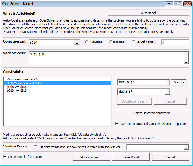
Once you have built your model, you can check it using OpenSolver’s “Show/Hide Model” button. This produces a display such as that shown above where the left hand side and right hand side of each constraint are boxed and joined, and the constraint sense indicated (being either ‘<‘ for ‘<=’, ‘>’ for ‘>=’, or ‘=’, where each constraint is read left-to-right and/or down the page). The objective (goal) cell is highlighted and tagged as either min (minimise) or max (maximise). The adjustable cells (decision variables) are shaded, with any integer variables being tagged with an ‘i’ and and binary variables with a ‘b’.

OpenSolver comes with a range of “solvers” designed for different types of optimisation problems; these are listed on our guide to solvers . To solve this linear model, choose a linear Solver such as CBC (which is the default solver), or Gurobi (if you have this commercial software installed), using OpenSovler’s Options button accessible from the OpenSolver Model menu. (You can also access this from the Model dialog.)

Note that OpenSolver does some checks that your model is a linear one, but it is up to you to ensure this is the case by avoiding functions such as sqrt(), if(), abs(), max(), min(), etc.

YouTube Videos of OpenSolver

You may wish to view this YouTube OpenSolver introduction by Kevin Jia ( Engineering Science department, University of Auckland )

or this YouTube movie showing the installation and use of OpenSolver :

This “ Solving Transportation Problems with OpenSolver ” page also includes a video.

Learn about Linear and Integer Programming

OpenSolver lets you solve linear and integer programming models. To find out more about these optimization models, you may wish to look at the online notes at Linear Programming – Foundations and Extensions . (This page did include a textbook by Robert Vanderbei, but this is no longer available. However, the lecture notes are still there.) Another online textbook is Decision Modelling by David Tullet , 2019 ( local copy ).

There is also a 2021 series of YouTube videos on modelling from Prof Dr Kimms ; these are not Excel-specific, but cover general modelling techniques.

Quick Solves

An advanced feature of OpenSolver is quick solving using ‘parameters’ that the user can change between solves. Building a large model is often much slower than solving the model. This can be very frustrating as users often need to solve the same model repeatedly after making changes to the constraint right hand sides. To handle this, OpenSolver allows you to define ‘parameter’ cells (using the “Set Quick Solve Parameters” menu) that are the cells you will be changing between successive solves. (These may be the actual right hand side cells, or other cells that determine the right hand side values.) You then choose the “Initialise Quick Solve”, at which point OpenSolver analyses your spreadsheet (which is has to do just once) to build the model and determine how your constraint right hand sides change as each parameter cell changes. OpenSolver assumes that this change is a linear one; it is up to you to make sure this is the case. You can then change your parameters, and click the Quick Solve button to very quickly solve the modified model. (See below for using Quick Solve from VBA.)

Solving the relaxation of an IP

OpenSolver provides a menu item to solve the relaxation of an integer program. This is often useful to understand how hard the problem will be to solve to optimality.

Extra Solver Parameters

OpenSolver allows the user to pass extra parameters to the solver by creating a named table on their spreadsheet. The table should have two columns, with a row for each solver option the user wants to set. The left column of each row should contain the name of the option (without any ‘-‘) and the associated right column should specify its value. You can then tell the solver to use these options by specifying this table as the `Extra Solver Parameters` range in the Options dialog.

See the reference guide for each solver to learn which parameters are supported:

Couenne (section 6)
NOMAD (sections 4.2 and 6)

Advanced CBC Control

Cbc logging.

If you are solving a large problem, then a useful extra parameters range for the CBC solver might look like the following. This turns on simplex and branch-and-bound logging; it will give you lots of output. Make sure you have used Model… Options… Show optimisation progress while solving to turn on display of CBC output.

Using CBC interactively

If you want to explore their problem directly with CBC, you can open a CBC command line window with the model loaded ready to be solved. Note that this does not allow solutions to be loaded back into Excel, but does allow different CBC options to be explored for use in subsequent solves by OpenSolver. This is useful if the problem takes a long time to build. To do this, select the OpenSolver… Open Last Model in CBC menu item.

If you wish to take control of CBC during an Excel run, then use the following as part of the extra parameter range:

The last parameter `-` with no value will cause CBC to enter interactive mode. Make sure you have used Model… Options… Show optimisation progress while solving to turn on display of CBC output. Then, after clicking OpenSolver’s Solver button, you will be at the CBC command prompt. Type: ‘stat’ to get a summary of your problem details, ‘solve’ to solve the problem, then ‘solution modelsolution.txt’ to write a solution, and ‘quit’ to return to Excel. OpenSolver will then load in the solution. This can be useful for debugging.

OpenSolver and Visual Basic for Applications (VBA)

OpenSolver can be called from your own VBA routines. To do this, in your VBA project you either need to add a reference to “OpenSolver” (or, as detailed below, use “Application.Run.) This site shows how to use the Tools menu to add OpenSolver as a Reference. Make sure you have opened OpenSolver before trying this. Then, you can take full control of OpenSolver using VBA with the functions listed here . OpenSolver is written in VBA, and so you can have a look at the code to see how it all works.

For example, you can run OpenSolver as follows:

Result will be one of the following: OpenSolverResult.ErrorOccurred, OpenSolverResult.Optimal, OpenSolverResult.Unbounded, OpenSolverResult.Infeasible, OpenSolverResult.TimeLimitedSubOptimal

Model Setup with VBA: We recommend that you set up the model on the spreadsheet in the normal way, and then in your VBA make any (presumably small) changes you want to the resulting spreadsheet (such as changing values on the spreadsheet that specify a constraint’s right hand side), and then call RunOpenSolver. If you really want to set up the whole model in VBA, then you should use the OpenSolver API functions to modify the model.

Note: As of OpenSolver 2.7.0 we strongly recommend you use the OpenSolver API instead of the Solver API detailed below. If you want to use the Solver API, after adding a reference to Solver, you can also use of the standard Solver VBA commands which are documented here . You can set up the model using these Solver commands, and then solve the resulting model using RunOpenSolver. If using the Solver API, we strongly suggest all references in your constraints are absolute (not relative) to avoid unpredictable behaviour (Thanks to Lukas for this feedback). This is not a problem with the OpenSolver API.

QuickSolve with VBA: To use Quick Solve from VBA, your code should look something like the following

See also the definitions of these function (in the API reference) for more fine-grained control of Quick Solve.

If there is a lot of demand for this feature, then we will look at making this VBA interface more powerful.

Running OpenSolver using Application.Run: If you include as reference to OpenSolver (as detailed above), then when you spreadsheet runs on another machine, OpenSolver has to be either in the same place on disk or already opened by the user. An alternative is not to add a reference, but run OpenSolver using Application.Run, as shown in the following code. This can be a good approach for sharing OpenSolver-based VBA solutions.

Disable dialogs for Application.Run:

Note that calling

with no additional arguments solves the model without hiding or disabling dialogs. If you want to repeatedly run OpenSolver and do not want to interact with forms OpenSolver might otherwise generate while running, then please replace the above line with:

or, if you want the result code, replace it with

If you need the result code (one of these OpenSolverResult values ), then use:

AddConstraint – model building using Application.Run with OpenSolver API

(Applies to Excel 2016 – other versions may differ)

When calling OpenSolver API subs and functions with the Application.Run method, normal VBA conventions about the scopes of subs and functions do not always apply. According to an article from wellsr and a StackOverflow question , Application.Run is able to run both ‘Public’ and ‘Private’ subs.

In OpenSolver.xlam, the sub AddConstraint is defined in two places – in the OpenSolverAPI module and the SolverFileNL module. Its definition in the API module is Public and in SolverFileNL it is Private.

However, if AddConstraint is called using Application.Run, it seems that these scopes are ignored and there are effectively conflicting or duplicate definitions for the sub – it is now ambiguous as to whether OpenSolverAPI.AddConstraint or SolverFileNL.AddConstraint should be run.

Thus, in order to build up a model using the OpenSolver API while using Application.Run, the following function call should be made e.g.:

instead of calling:

Optimizing the output of VBA macros with NOMAD

It is possible to optimize the results of a VBA macro if you are using the NOMAD solver. An example of where this might be desirable would be if the objective/constraints in your model depend on a PivotTable related to the variable values, since PivotTables are not updated when the sheet is recalculated. For another example, see our announcement post about this feature where it is used to optimize the parameters controlling an ODE simulation.

To use this feature, you must create a macro to be used as the “callback” function. This macro will be called at each iteration of the optimization after the new variable values have been set on the sheet, and it should update the parts of the sheet that depend on these new values. The macro should be a Sub that takes no parameters. You must specify the name of the callback macro using the “Extra Solver Parameters” feature described above with the parameter name “OpenSolver_Callback”. The name of the callback must be prefixed with the name of the workbook (quoted if there is a space in the name). An example of how the Extra Solver Parameters range might look for a macro called “mymacro” in a file called “test.xlsm” is below:

Cancelling the solve from inside the callback macro

If you want to cancel the solve process from inside you callback macro while the solve is progressing (e.g. if the escape button is pressed), you can trigger this by calling the VBA function “OpenSolver.NOMAD_CallbackAbort”, which will prompt the user to confirm cancelling the solve. Our suggested format for incorporating this into your callback macro is something following the code snippet below, which runs a macro called “updateObjective”, and prompts the user to cancel if the escape button is pressed during the solve:

We have provided an example workbook that uses this feature here in order to demonstrate how to properly use this advanced feature.

The Excel Solver is a product developed by Frontline Systems for Microsoft. OpenSolver has no affiliation with, nor is recommend by, Microsoft or Frontline Systems. All trademark terms are the property of their respective owners.

One thought on “Using OpenSolver”

Pingback: OpenSolver 2.6.1 (15 Feb 2015) « OpenSolver for Excel

Comments are closed.

IMAGES

How to Solve Integer Linear Programming in Excel (With Easy Steps)
Excel
Integer Linear Programming: Excel Solver Example 1
Excel: How to solve Integer Programming in excel using excel solver -LP-OR -Operational Research
Integer Programming: Set Covering with Excel Solver
Integer programming excel solver examples

VIDEO

Excel: How to solve Integer Programming in excel using excel solver -LP-OR -Operational Research
MBA 6010P: Integer Linear Programming III
Lecture 05 09 Various Uses of Binary Integer Programming Excel Solver
Introduction to Solver for Numerical Solutions in Microsoft Excel
Tutorial: Solver Excel
MBA 6010P: Integer Linear Programming II

COMMENTS

How to Solve Integer Linear Programming in Excel (With Easy Steps)
STEP 2: Load Solver Add-in in Excel. Secondly, we need to load the Solver add-in in Excel. If it is already loaded in your Excel, then, you can move forward to step 3. To do so, click on the File tab. After that, select Options from the left - bottom corner of the screen. It will open the Excel Options window.
Excel Solver tutorial with step-by-step examples
To add Solver to your Excel, perform the following steps: In Excel 2010 - Excel 365, click File > Options. In Excel 2007, click the Microsoft Office button, and then click Excel Options. In the Excel Options dialog, click Add-Ins on the left sidebar, make sure Excel Add-ins is selected in the Manage box at the bottom of the window, and click Go ...
Excel Solver
When a Solver model includes integer, binary or alldifferent constraints, it is called an integer programming problem. Integer constraints make a model non-convex, and finding the optimal solution to an integer programming problem is equivalent to solving a global optimization problem. Such problems may require far more computing time than the same problem without the integer constraints.
Define and solve a problem by using Solver
Solver is a Microsoft Excel add-in program you can use for what-if analysis. Use Solver to find an optimal (maximum or minimum) value for a formula in one cell — called the objective cell — subject to constraints, or limits, on the values of other formula cells on a worksheet. Solver works with a group of cells, called decision variables or ...
Excel
ISM Course ExcelPart 11.05The corresponding playlist can be found here: Excel (en): https://www.youtube.com/playlist?list=PL0eGlOnA3oppM0mxuLqYW6-TqR2NlZrZXA...
Optimization Modeling with Solver in Excel • Stephen L. Nelson
To install Solver, choose the Tools menu's Add-Ins command. When Excel displays the Add-Ins dialog box, scroll down the Add-Ins Available list box until you see the Solver Add-In entry. Select the Solver Add-In check box, click OK, and then if Excel requests it, provide the Excel or Office installation CD. Figure 6-18.
Integer Programming: Set Covering with Excel Solver
Enjoyed this content & want to support my channel? You can get the spreadsheet I build in the video or buy me a coffee! Links below:Buy me a coffee: https://...
Integer Linear Programming: Excel Solver Example 1
An ILP example using Excel Solver.
Excel Solver
Go to File: Click on the "File" tab in the top left corner. Select Options: Choose "Options" from the drop-down menu. Choose Add-ins: In the Excel Options window, click on "Add-ins". Manage Add-ins: At the bottom of this window, find the "Manage" box. Select "Excel Add-ins" and click "Go". 6. Enable Solver: Check the box ...
PDF Using Excel to solve linear programming problems
Subject to the constraints: Click on Add. Click on Cell Reference and then click in D15, then click on Constraint and then click in F15. Be sure the test listed between them is <=. Now click on Options. Make sure Assume Linear Model and. Assume Non-Negative boxes are checked, then click OK. Back at the Solver, click Solve.
PDF Integer Programming
IPs. In Section 9.2, we explain how to formulate integer programming models. We also dis-cuss how to solve IPs on the computer with LINDO, LINGO, and Excel Solver. In Sections 9.3-9.8, we discuss other methods used to solve IPs. 9.1 Introduction to Integer Programming An IP in which all variables are required to be integers is called a pure ...
Excel Solver
The Ignore Integer Constraints check box allows you to solve the "relaxation" of an integer programming problem, where the integer, binary, and alldifferent constraints are ignored, but all other constraints are enforced. The Integer Optimality (%) option, sometimes called the "MIP gap", allows Solver to stop if it finds an integer ...
PDF Excel Solver
• Excel has the capability to solve linear (and often nonlinear) programming problems with the SOLVER tool, which: - May be used to solve linear and nonlinear optimization problems - Allows integer or binary restrictions to be placed on decision variables - Can be used to solve problems with up to 200 decision variables • SOLVER is an ...
Using Solver to determine the optimal product mix
To begin, click the Data tab, and in the Analysis group, click Solver. Note: As explained in Chapter 26, "An Introduction to Optimization with Excel Solver," Solver is installed by clicking the Microsoft Office Button, then Excel Options, followed by Add-Ins. In the Manage list, click Excel Add-ins, check the Solver Add-in box, and then click ...
Introducing Integer Modeling with Excel Solver
Extending the linear programming model to an integer programming model happens as follows: cells D12:F12 are specified as "bin" (binary) in the constraints part of the Solver dialog box, and added to the changing cells part in the Solver dialog box. At the beginning, I leave the option "Assume Linear Model" unchecked.
Excel Solver Tutorial
Product Mix Example - Using Excel's Built-In Solver Using the Solver Dialogs To let the Solver know which cells on the worksheet represent the decision variables, constraints and objective function, we click Solver button on the Data tab, or the Premium Solver button on the Add-Ins tab, which displays the Solver Parameters dialog. In the Set Objective (or Set Target Cell) edit box, we type or ...
Solve problems with linear programming and Excel
Linear programming, as demonstrated by applying Excel's Solver feature, is a viable and cost-effective tool for analysing multi-variable financial and operational problems. In the example, it was unclear at the outset what the optimal production quantity of each washing machine was given the stated objective of profit maximisation.
ORMM Excel
The Solver Add-in comes with Excel, and it can solve linear programming, integer programming and nonlinear programming models. Additional add-ins are available in this package to solve linear programming, integer programming, network programming and transportation models. Add-in - Click the add-in name to download a zipped .xla file.
Excel: How to solve Integer Programming in excel using excel solver -LP
Excel: How to solve Integer Programming in excel using excel solver. Linear Programming - OR -Operational Research (United Kingdom - UK) - Operations Resea...
Linear Programming with Spreadsheets
Linear Programming Example. Objective function: Max Z: 250 X + 75 Y. Subjected to constraints: 5 * X + Y <= 100, X + Y <= 60 and Where X,Y >= 0 Step 1: Let's write the function in excel like shown below. Step 2: After writing objective function and constraints in the spreadsheet, let's calculate values for constraints C1 and C2. You can ...
Integer Programming: Logical Conditions with Binary Variables in Excel
Enjoyed this content & want to support my channel? You can get the spreadsheet I build in the video or buy me a coffee! Links below:Buy me a coffee: https://...
Using OpenSolver
This "Solving Transportation Problems with OpenSolver" page also includes a video. Learn about Linear and Integer Programming. OpenSolver lets you solve linear and integer programming models. To find out more about these optimization models, you may wish to look at the online notes at Linear Programming - Foundations and Extensions. (This page did include a textbook by Robert Vanderbei ...