This is “Solving Systems of Linear Inequalities (Two Variables)”, section 4.5 from the book Beginning Algebra (v. 1.0). For details on it (including licensing), click here .
This book is licensed under a Creative Commons by-nc-sa 3.0 license. See the license for more details, but that basically means you can share this book as long as you credit the author (but see below), don't make money from it, and do make it available to everyone else under the same terms.
This content was accessible as of December 29, 2012, and it was downloaded then by Andy Schmitz in an effort to preserve the availability of this book.
Normally, the author and publisher would be credited here. However, the publisher has asked for the customary Creative Commons attribution to the original publisher, authors, title, and book URI to be removed. Additionally, per the publisher's request, their name has been removed in some passages. More information is available on this project's attribution page .
For more information on the source of this book, or why it is available for free, please see the project's home page . You can browse or download additional books there. To download a .zip file containing this book to use offline, simply click here .

4.5 Solving Systems of Linear Inequalities (Two Variables)
Learning objectives.
- Check solutions to systems of linear inequalities with two variables.
- Solve systems of linear inequalities.
Solutions to Systems of Linear Inequalities
A system of linear inequalities A set of two or more linear inequalities that define the conditions to be considered simultaneously. consists of a set of two or more linear inequalities with the same variables. The inequalities define the conditions that are to be considered simultaneously. For example,

We know that each inequality in the set contains infinitely many ordered pair solutions defined by a region in a rectangular coordinate plane. When considering two of these inequalities together, the intersection of these sets defines the set of simultaneous ordered pair solutions. When we graph each of the above inequalities separately, we have

When graphed on the same set of axes, the intersection can be determined.

The intersection is shaded darker and the final graph of the solution set is presented as follows:

The graph suggests that (3, 2) is a solution because it is in the intersection. To verify this, show that it solves both of the original inequalities:

Points on the solid boundary are included in the set of simultaneous solutions and points on the dashed boundary are not. Consider the point (−1, 0) on the solid boundary defined by y = 2 x + 2 and verify that it solves the original system:

Notice that this point satisfies both inequalities and thus is included in the solution set. Now consider the point (2, 0) on the dashed boundary defined by y = x − 2 and verify that it does not solve the original system:

This point does not satisfy both inequalities and thus is not included in the solution set.
Solving Systems of Linear Inequalities
Solutions to a system of linear inequalities are the ordered pairs that solve all the inequalities in the system. Therefore, to solve these systems, graph the solution sets of the inequalities on the same set of axes and determine where they intersect. This intersection, or overlap, defines the region of common ordered pair solutions.
Example 1: Graph the solution set: { − 2 x + y > − 4 3 x − 6 y ≥ 6 .
Solution: To facilitate the graphing process, we first solve for y .

For the first inequality, we use a dashed boundary defined by y = 2 x − 4 and shade all points above the line. For the second inequality, we use a solid boundary defined by y = 1 2 x − 1 and shade all points below. The intersection is darkened.

Now we present the solution with only the intersection shaded.

Example 2: Graph the solution set: { − 2 x + 3 y > 6 4 x − 6 y > 12 .
Solution: Begin by solving both inequalities for y .

Use a dashed line for each boundary. For the first inequality, shade all points above the boundary. For the second inequality, shade all points below the boundary.

As you can see, there is no intersection of these two shaded regions. Therefore, there are no simultaneous solutions.
Answer: No solution, ∅
Example 3: Graph the solution set: { y ≥ − 4 y < x + 3 y ≤ − 3 x + 3 .
Solution: The intersection of all the shaded regions forms the triangular region as pictured darkened below:

After graphing all three inequalities on the same set of axes, we determine that the intersection lies in the triangular region pictured.

The graphic suggests that (−1, 1) is a common point. As a check, substitute that point into the inequalities and verify that it solves all three conditions.

Key Takeaway
- To solve systems of linear inequalities, graph the solution sets of each inequality on the same set of axes and determine where they intersect.
Topic Exercises
Part A: Solving Systems of Linear Inequalities
Determine whether the given point is a solution to the given system of linear equations.
1. (3, 2); { y ≤ x + 3 y ≥ − x + 3
2. (−3, −2); { y < − 3 x + 4 y ≥ 2 x − 1
3. (5, 0); { y > − x + 5 y ≤ 3 4 x − 2
4. (0, 1); { y < 2 3 x + 1 y ≥ 5 2 x − 2
5. ( − 1 , 8 3 ) ; { − 4 x + 3 y ≥ − 12 2 x + 3 y < 6
6. (−1, −2); { − x + y < 0 x + y < 0 x + y < − 2
Part B: Solving Systems of Linear Inequalities
Graph the solution set.
7. { y ≤ x + 3 y ≥ − x + 3
8. { y < − 3 x + 4 y ≥ 2 x − 1
9. { y > x y < − 1
10. { y < 2 3 x + 1 y ≥ 5 2 x − 2
11. { y > − x + 5 y ≤ 3 4 x − 2
12. { y > 3 5 x + 3 y < 3 5 x − 3
13. { x + 4 y < 12 − 3 x + 12 y ≥ − 12
14. { − x + y ≤ 6 2 x + y ≥ 1
15. { − 2 x + 3 y > 3 4 x − 3 y < 15
16. { − 4 x + 3 y ≥ − 12 2 x + 3 y < 6
17. { 5 x + y ≤ 4 − 4 x + 3 y < − 6
18. { 3 x + 5 y < 15 − x + 2 y ≤ 0
19. { x ≥ 0 5 x + y > 5
20. { x ≥ − 2 y ≥ 1
21. { x − 3 < 0 y + 2 ≥ 0
22. { 5 y ≥ 2 x + 5 − 2 x < − 5 y − 5
23. { x − y ≥ 0 − x + y < 1
24. { − x + y ≥ 0 y − x < 1
25. { x > − 2 x ≤ 2
26. { y > − 1 y < 2
27. { − x + 2 y > 8 3 x − 6 y ≥ 18
28. { − 3 x + 4 y ≤ 4 6 x − 8 y > − 8
29. { 2 x + y < 3 − x ≤ 1 2 y
30. { 2 x + 6 y ≤ 6 − 1 3 x − y ≤ 3
31. { y < 3 y > x x > − 4
32. { y < 1 y ≥ x − 1 y < − 3 x + 3
33. { − 4 x + 3 y > − 12 y ≥ 2 2 x + 3 y > 6
34. { − x + y < 0 x + y ≤ 0 x + y > − 2
35. { x + y < 2 x < 3 − x + y ≤ 2
36. { y + 4 ≥ 0 1 2 x + 1 3 y ≤ 1 − 1 2 x + 1 3 y ≤ 1
37. Construct a system of linear inequalities that describes all points in the first quadrant.
38. Construct a system of linear inequalities that describes all points in the second quadrant.
39. Construct a system of linear inequalities that describes all points in the third quadrant.
40. Construct a system of linear inequalities that describes all points in the fourth quadrant.

27: No solution, ∅

37: { x > 0 y > 0
39: { x < 0 y < 0
7.1 Systems of Linear Equations: Two Variables
Learning objectives.
In this section, you will:
- Solve systems of equations by graphing.
- Solve systems of equations by substitution.
- Solve systems of equations by addition.
- Identify inconsistent systems of equations containing two variables.
- Express the solution of a system of dependent equations containing two variables.
A skateboard manufacturer introduces a new line of boards. The manufacturer tracks its costs, which is the amount it spends to produce the boards, and its revenue, which is the amount it earns through sales of its boards. How can the company determine if it is making a profit with its new line? How many skateboards must be produced and sold before a profit is possible? In this section, we will consider linear equations with two variables to answer these and similar questions.
Introduction to Systems of Equations
In order to investigate situations such as that of the skateboard manufacturer, we need to recognize that we are dealing with more than one variable and likely more than one equation. A system of linear equations consists of two or more linear equations made up of two or more variables such that all equations in the system are considered simultaneously. To find the unique solution to a system of linear equations, we must find a numerical value for each variable in the system that will satisfy all equations in the system at the same time. Some linear systems may not have a solution and others may have an infinite number of solutions. In order for a linear system to have a unique solution, there must be at least as many equations as there are variables. Even so, this does not guarantee a unique solution.
In this section, we will look at systems of linear equations in two variables, which consist of two equations that contain two different variables. For example, consider the following system of linear equations in two variables.
The solution to a system of linear equations in two variables is any ordered pair that satisfies each equation independently. In this example, the ordered pair (4, 7) is the solution to the system of linear equations. We can verify the solution by substituting the values into each equation to see if the ordered pair satisfies both equations. Shortly we will investigate methods of finding such a solution if it exists.
In addition to considering the number of equations and variables, we can categorize systems of linear equations by the number of solutions. A consistent system of equations has at least one solution. A consistent system is considered to be an independent system if it has a single solution, such as the example we just explored. The two lines have different slopes and intersect at one point in the plane. A consistent system is considered to be a dependent system if the equations have the same slope and the same y -intercepts. In other words, the lines coincide so the equations represent the same line. Every point on the line represents a coordinate pair that satisfies the system. Thus, there are an infinite number of solutions.
Another type of system of linear equations is an inconsistent system , which is one in which the equations represent two parallel lines. The lines have the same slope and different y- intercepts. There are no points common to both lines; hence, there is no solution to the system.
Types of Linear Systems
There are three types of systems of linear equations in two variables, and three types of solutions.
- An independent system has exactly one solution pair ( x , y ) . ( x , y ) . The point where the two lines intersect is the only solution.
- An inconsistent system has no solution. Notice that the two lines are parallel and will never intersect.
- A dependent system has infinitely many solutions. The lines are coincident. They are the same line, so every coordinate pair on the line is a solution to both equations.
Figure 2 compares graphical representations of each type of system.
Given a system of linear equations and an ordered pair, determine whether the ordered pair is a solution.
- Substitute the ordered pair into each equation in the system.
- Determine whether true statements result from the substitution in both equations; if so, the ordered pair is a solution.
Determining Whether an Ordered Pair Is a Solution to a System of Equations
Determine whether the ordered pair ( 5 , 1 ) ( 5 , 1 ) is a solution to the given system of equations.
Substitute the ordered pair ( 5 , 1 ) ( 5 , 1 ) into both equations.
The ordered pair ( 5 , 1 ) ( 5 , 1 ) satisfies both equations, so it is the solution to the system.
We can see the solution clearly by plotting the graph of each equation. Since the solution is an ordered pair that satisfies both equations, it is a point on both of the lines and thus the point of intersection of the two lines. See Figure 3 .
Determine whether the ordered pair ( 8 , 5 ) ( 8 , 5 ) is a solution to the following system.
Solving Systems of Equations by Graphing
There are multiple methods of solving systems of linear equations. For a system of linear equations in two variables, we can determine both the type of system and the solution by graphing the system of equations on the same set of axes.
Solving a System of Equations in Two Variables by Graphing
Solve the following system of equations by graphing. Identify the type of system.
Solve the first equation for y . y .
Solve the second equation for y . y .
Graph both equations on the same set of axes as in Figure 4 .
The lines appear to intersect at the point ( −3, −2 ) . ( −3, −2 ) . We can check to make sure that this is the solution to the system by substituting the ordered pair into both equations.
The solution to the system is the ordered pair ( −3, −2 ) , ( −3, −2 ) , so the system is independent.
Solve the following system of equations by graphing.
Can graphing be used if the system is inconsistent or dependent?
Yes, in both cases we can still graph the system to determine the type of system and solution. If the two lines are parallel, the system has no solution and is inconsistent. If the two lines are identical, the system has infinite solutions and is a dependent system.
Solving Systems of Equations by Substitution
Solving a linear system in two variables by graphing works well when the solution consists of integer values, but if our solution contains decimals or fractions, it is not the most precise method. We will consider two more methods of solving a system of linear equations that are more precise than graphing. One such method is solving a system of equations by the substitution method , in which we solve one of the equations for one variable and then substitute the result into the second equation to solve for the second variable. Recall that we can solve for only one variable at a time, which is the reason the substitution method is both valuable and practical.
Given a system of two equations in two variables, solve using the substitution method.
- Solve one of the two equations for one of the variables in terms of the other.
- Substitute the expression for this variable into the second equation, then solve for the remaining variable.
- Substitute that solution into either of the original equations to find the value of the first variable. If possible, write the solution as an ordered pair.
- Check the solution in both equations.
Solving a System of Equations in Two Variables by Substitution
Solve the following system of equations by substitution.
First, we will solve the first equation for y . y .
Now we can substitute the expression x −5 x −5 for y y in the second equation.
Now, we substitute x = 8 x = 8 into the first equation and solve for y . y .
Our solution is ( 8 , 3 ) . ( 8 , 3 ) .
Check the solution by substituting ( 8 , 3 ) ( 8 , 3 ) into both equations.
Can the substitution method be used to solve any linear system in two variables?
Yes, but the method works best if one of the equations contains a coefficient of 1 or –1 so that we do not have to deal with fractions.
Solving Systems of Equations in Two Variables by the Addition Method
A third method of solving systems of linear equations is the addition method . In this method, we add two terms with the same variable, but opposite coefficients, so that the sum is zero. Of course, not all systems are set up with the two terms of one variable having opposite coefficients. Often we must adjust one or both of the equations by multiplication so that one variable will be eliminated by addition.
Given a system of equations, solve using the addition method.
- Write both equations with x - and y -variables on the left side of the equal sign and constants on the right.
- Write one equation above the other, lining up corresponding variables. If one of the variables in the top equation has the opposite coefficient of the same variable in the bottom equation, add the equations together, eliminating one variable. If not, use multiplication by a nonzero number so that one of the variables in the top equation has the opposite coefficient of the same variable in the bottom equation, then add the equations to eliminate the variable.
- Solve the resulting equation for the remaining variable.
- Substitute that value into one of the original equations and solve for the second variable.
- Check the solution by substituting the values into the other equation.
Solving a System by the Addition Method
Solve the given system of equations by addition.
Both equations are already set equal to a constant. Notice that the coefficient of x x in the second equation, –1, is the opposite of the coefficient of x x in the first equation, 1. We can add the two equations to eliminate x x without needing to multiply by a constant.
Now that we have eliminated x , x , we can solve the resulting equation for y . y .
Then, we substitute this value for y y into one of the original equations and solve for x . x .
The solution to this system is ( − 7 3 , 2 3 ) . ( − 7 3 , 2 3 ) .
Check the solution in the first equation.
We gain an important perspective on systems of equations by looking at the graphical representation. See Figure 5 to find that the equations intersect at the solution. We do not need to ask whether there may be a second solution because observing the graph confirms that the system has exactly one solution.
Using the Addition Method When Multiplication of One Equation Is Required
Solve the given system of equations by the addition method .
Adding these equations as presented will not eliminate a variable. However, we see that the first equation has 3 x 3 x in it and the second equation has x . x . So if we multiply the second equation by −3 , −3 , the x -terms will add to zero.
Now, let’s add them.
For the last step, we substitute y = −4 y = −4 into one of the original equations and solve for x . x .
Our solution is the ordered pair ( 3 , −4 ) . ( 3 , −4 ) . See Figure 6 . Check the solution in the original second equation.
Solve the system of equations by addition.
Using the Addition Method When Multiplication of Both Equations Is Required
Solve the given system of equations in two variables by addition.
One equation has 2 x 2 x and the other has 5 x . 5 x . The least common multiple is 10 x 10 x so we will have to multiply both equations by a constant in order to eliminate one variable. Let’s eliminate x x by multiplying the first equation by −5 −5 and the second equation by 2. 2.
Then, we add the two equations together.
Substitute y = −4 y = −4 into the original first equation.
The solution is ( −2 , −4 ) . ( −2 , −4 ) . Check it in the other equation.
See Figure 7 .
Using the Addition Method in Systems of Equations Containing Fractions
First clear each equation of fractions by multiplying both sides of the equation by the least common denominator.
Now multiply the second equation by −1 −1 so that we can eliminate the x -variable.
Add the two equations to eliminate the x -variable and solve the resulting equation.
Substitute y = 7 y = 7 into the first equation.
The solution is ( 11 2 , 7 ) . ( 11 2 , 7 ) . Check it in the other equation.
Identifying Inconsistent Systems of Equations Containing Two Variables
Now that we have several methods for solving systems of equations, we can use the methods to identify inconsistent systems. Recall that an inconsistent system consists of parallel lines that have the same slope but different y y -intercepts. They will never intersect. When searching for a solution to an inconsistent system, we will come up with a false statement, such as 12 = 0. 12 = 0.
Solving an Inconsistent System of Equations
Solve the following system of equations.
We can approach this problem in two ways. Because one equation is already solved for x , x , the most obvious step is to use substitution.
Clearly, this statement is a contradiction because 9 ≠ 13. 9 ≠ 13. Therefore, the system has no solution.
The second approach would be to first manipulate the equations so that they are both in slope-intercept form. We manipulate the first equation as follows.
We then convert the second equation expressed to slope-intercept form.
Comparing the equations, we see that they have the same slope but different y -intercepts. Therefore, the lines are parallel and do not intersect.
Writing the equations in slope-intercept form confirms that the system is inconsistent because all lines will intersect eventually unless they are parallel. Parallel lines will never intersect; thus, the two lines have no points in common. The graphs of the equations in this example are shown in Figure 8 .
Solve the following system of equations in two variables.
Expressing the Solution of a System of Dependent Equations Containing Two Variables
Recall that a dependent system of equations in two variables is a system in which the two equations represent the same line. Dependent systems have an infinite number of solutions because all of the points on one line are also on the other line. After using substitution or addition, the resulting equation will be an identity, such as 0 = 0. 0 = 0.
Finding a Solution to a Dependent System of Linear Equations
Find a solution to the system of equations using the addition method .
With the addition method, we want to eliminate one of the variables by adding the equations. In this case, let’s focus on eliminating x . x . If we multiply both sides of the first equation by −3 , −3 , then we will be able to eliminate the x x -variable.
Now add the equations.
We can see that there will be an infinite number of solutions that satisfy both equations.
If we rewrote both equations in the slope-intercept form, we might know what the solution would look like before adding. Let’s look at what happens when we convert the system to slope-intercept form.
See Figure 9 . Notice the results are the same. The general solution to the system is ( x , − 1 3 x + 2 3 ) . ( x , − 1 3 x + 2 3 ) .
Using Systems of Equations to Investigate Profits
Using what we have learned about systems of equations, we can return to the skateboard manufacturing problem at the beginning of the section. The skateboard manufacturer’s revenue function is the function used to calculate the amount of money that comes into the business. It can be represented by the equation R = x p , R = x p , where x = x = quantity and p = p = price. The revenue function is shown in orange in Figure 10 .
The cost function is the function used to calculate the costs of doing business. It includes fixed costs, such as rent and salaries, and variable costs, such as utilities. The cost function is shown in blue in Figure 10 . The x x -axis represents quantity in hundreds of units. The y -axis represents either cost or revenue in hundreds of dollars.
The point at which the two lines intersect is called the break-even point . We can see from the graph that if 700 units are produced, the cost is $3,300 and the revenue is also $3,300. In other words, the company breaks even if they produce and sell 700 units. They neither make money nor lose money.
The shaded region to the right of the break-even point represents quantities for which the company makes a profit. The shaded region to the left represents quantities for which the company suffers a loss. The profit function is the revenue function minus the cost function, written as P ( x ) = R ( x ) − C ( x ) . P ( x ) = R ( x ) − C ( x ) . Clearly, knowing the quantity for which the cost equals the revenue is of great importance to businesses.
Finding the Break-Even Point and the Profit Function Using Substitution
Given the cost function C ( x ) = 0.85 x + 35,000 C ( x ) = 0.85 x + 35,000 and the revenue function R ( x ) = 1.55 x , R ( x ) = 1.55 x , find the break-even point and the profit function.
Write the system of equations using y y to replace function notation.
Substitute the expression 0.85 x + 35,000 0.85 x + 35,000 from the first equation into the second equation and solve for x . x .
Then, we substitute x = 50,000 x = 50,000 into either the cost function or the revenue function.
The break-even point is ( 50,000 , 77,500 ) . ( 50,000 , 77,500 ) .
The profit function is found using the formula P ( x ) = R ( x ) − C ( x ) . P ( x ) = R ( x ) − C ( x ) .
The profit function is P ( x ) = 0.7 x −35,000. P ( x ) = 0.7 x −35,000.
The cost to produce 50,000 units is $77,500, and the revenue from the sales of 50,000 units is also $77,500. To make a profit, the business must produce and sell more than 50,000 units. See Figure 11 .
We see from the graph in Figure 12 that the profit function has a negative value until x = 50,000 , x = 50,000 , when the graph crosses the x -axis. Then, the graph emerges into positive y -values and continues on this path as the profit function is a straight line. This illustrates that the break-even point for businesses occurs when the profit function is 0. The area to the left of the break-even point represents operating at a loss.
Writing and Solving a System of Equations in Two Variables
The cost of a ticket to the circus is $ 25.00 $ 25.00 for children and $ 50.00 $ 50.00 for adults. On a certain day, attendance at the circus is 2,000 2,000 and the total gate revenue is $ 70,000. $ 70,000. How many children and how many adults bought tickets?
Let c = the number of children and a = the number of adults in attendance.
The total number of people is 2,000. 2,000. We can use this to write an equation for the number of people at the circus that day.
The revenue from all children can be found by multiplying $ 25.00 $ 25.00 by the number of children, 25 c . 25 c . The revenue from all adults can be found by multiplying $ 50.00 $ 50.00 by the number of adults, 50 a . 50 a . The total revenue is $ 70,000. $ 70,000. We can use this to write an equation for the revenue.
We now have a system of linear equations in two variables.
In the first equation, the coefficient of both variables is 1. We can quickly solve the first equation for either c c or a . a . We will solve for a . a .
Substitute the expression 2,000 − c 2,000 − c in the second equation for a a and solve for c . c .
Substitute c = 1,200 c = 1,200 into the first equation to solve for a . a .
We find that 1,200 1,200 children and 800 800 adults bought tickets to the circus that day.
Meal tickets at the circus cost $ 4.00 $ 4.00 for children and $ 12.00 $ 12.00 for adults. If 1,650 1,650 meal tickets were bought for a total of $ 14,200 , $ 14,200 , how many children and how many adults bought meal tickets?
Access these online resources for additional instruction and practice with systems of linear equations.
- Solving Systems of Equations Using Substitution
- Solving Systems of Equations Using Elimination
- Applications of Systems of Equations
7.1 Section Exercises
Can a system of linear equations have exactly two solutions? Explain why or why not.
If you are performing a break-even analysis for a business and their cost and revenue equations are dependent, explain what this means for the company’s profit margins.
If you are solving a break-even analysis and get a negative break-even point, explain what this signifies for the company?
If you are solving a break-even analysis and there is no break-even point, explain what this means for the company. How should they ensure there is a break-even point?
Given a system of equations, explain at least two different methods of solving that system.
For the following exercises, determine whether the given ordered pair is a solution to the system of equations.
5 x − y = 4 x + 6 y = 2 5 x − y = 4 x + 6 y = 2 and ( 4 , 0 ) ( 4 , 0 )
−3 x − 5 y = 13 − x + 4 y = 10 −3 x − 5 y = 13 − x + 4 y = 10 and ( −6 , 1 ) ( −6 , 1 )
3 x + 7 y = 1 2 x + 4 y = 0 3 x + 7 y = 1 2 x + 4 y = 0 and ( 2 , 3 ) ( 2 , 3 )
−2 x + 5 y = 7 2 x + 9 y = 7 −2 x + 5 y = 7 2 x + 9 y = 7 and ( −1 , 1 ) ( −1 , 1 )
x + 8 y = 43 3 x −2 y = −1 x + 8 y = 43 3 x −2 y = −1 and ( 3 , 5 ) ( 3 , 5 )
For the following exercises, solve each system by substitution.
x + 3 y = 5 2 x + 3 y = 4 x + 3 y = 5 2 x + 3 y = 4
3 x −2 y = 18 5 x + 10 y = −10 3 x −2 y = 18 5 x + 10 y = −10
4 x + 2 y = −10 3 x + 9 y = 0 4 x + 2 y = −10 3 x + 9 y = 0
2 x + 4 y = −3.8 9 x −5 y = 1.3 2 x + 4 y = −3.8 9 x −5 y = 1.3
− 2 x + 3 y = 1.2 − 3 x − 6 y = 1.8 − 2 x + 3 y = 1.2 − 3 x − 6 y = 1.8
x −0.2 y = 1 −10 x + 2 y = 5 x −0.2 y = 1 −10 x + 2 y = 5
3 x + 5 y = 9 30 x + 50 y = −90 3 x + 5 y = 9 30 x + 50 y = −90
−3 x + y = 2 12 x −4 y = −8 −3 x + y = 2 12 x −4 y = −8
1 2 x + 1 3 y = 16 1 6 x + 1 4 y = 9 1 2 x + 1 3 y = 16 1 6 x + 1 4 y = 9
− 1 4 x + 3 2 y = 11 − 1 8 x + 1 3 y = 3 − 1 4 x + 3 2 y = 11 − 1 8 x + 1 3 y = 3
For the following exercises, solve each system by addition.
−2 x + 5 y = −42 7 x + 2 y = 30 −2 x + 5 y = −42 7 x + 2 y = 30
6 x −5 y = −34 2 x + 6 y = 4 6 x −5 y = −34 2 x + 6 y = 4
5 x − y = −2.6 −4 x −6 y = 1.4 5 x − y = −2.6 −4 x −6 y = 1.4
7 x −2 y = 3 4 x + 5 y = 3.25 7 x −2 y = 3 4 x + 5 y = 3.25
−x + 2 y = −1 5 x −10 y = 6 −x + 2 y = −1 5 x −10 y = 6
7 x + 6 y = 2 −28 x −24 y = −8 7 x + 6 y = 2 −28 x −24 y = −8
5 6 x + 1 4 y = 0 1 8 x − 1 2 y = − 43 120 5 6 x + 1 4 y = 0 1 8 x − 1 2 y = − 43 120
1 3 x + 1 9 y = 2 9 − 1 2 x + 4 5 y = − 1 3 1 3 x + 1 9 y = 2 9 − 1 2 x + 4 5 y = − 1 3
−0.2 x + 0.4 y = 0.6 x −2 y = −3 −0.2 x + 0.4 y = 0.6 x −2 y = −3
−0.1 x + 0.2 y = 0.6 5 x −10 y = 1 −0.1 x + 0.2 y = 0.6 5 x −10 y = 1
For the following exercises, solve each system by any method.
5 x + 9 y = 16 x + 2 y = 4 5 x + 9 y = 16 x + 2 y = 4
6 x −8 y = −0.6 3 x + 2 y = 0.9 6 x −8 y = −0.6 3 x + 2 y = 0.9
5 x −2 y = 2.25 7 x −4 y = 3 5 x −2 y = 2.25 7 x −4 y = 3
x − 5 12 y = − 55 12 −6 x + 5 2 y = 55 2 x − 5 12 y = − 55 12 −6 x + 5 2 y = 55 2
7 x −4 y = 7 6 2 x + 4 y = 1 3 7 x −4 y = 7 6 2 x + 4 y = 1 3
3 x + 6 y = 11 2 x + 4 y = 9 3 x + 6 y = 11 2 x + 4 y = 9
7 3 x − 1 6 y = 2 − 21 6 x + 3 12 y = −3 7 3 x − 1 6 y = 2 − 21 6 x + 3 12 y = −3
1 2 x + 1 3 y = 1 3 3 2 x + 1 4 y = − 1 8 1 2 x + 1 3 y = 1 3 3 2 x + 1 4 y = − 1 8
2.2 x + 1.3 y = −0.1 4.2 x + 4.2 y = 2.1 2.2 x + 1.3 y = −0.1 4.2 x + 4.2 y = 2.1
0.1 x + 0.2 y = 2 0.35 x −0.3 y = 0 0.1 x + 0.2 y = 2 0.35 x −0.3 y = 0
For the following exercises, graph the system of equations and state whether the system is consistent, inconsistent, or dependent and whether the system has one solution, no solution, or infinite solutions.
3 x − y = 0.6 x −2 y = 1.3 3 x − y = 0.6 x −2 y = 1.3
− x + 2 y = 4 2 x −4 y = 1 − x + 2 y = 4 2 x −4 y = 1
x + 2 y = 7 2 x + 6 y = 12 x + 2 y = 7 2 x + 6 y = 12
3 x −5 y = 7 x −2 y = 3 3 x −5 y = 7 x −2 y = 3
3 x −2 y = 5 −9 x + 6 y = −15 3 x −2 y = 5 −9 x + 6 y = −15
For the following exercises, use the intersect function on a graphing device to solve each system. Round all answers to the nearest hundredth.
0.1 x + 0.2 y = 0.3 −0.3 x + 0.5 y = 1 0.1 x + 0.2 y = 0.3 −0.3 x + 0.5 y = 1
−0.01 x + 0.12 y = 0.62 0.15 x + 0.20 y = 0.52 −0.01 x + 0.12 y = 0.62 0.15 x + 0.20 y = 0.52
0.5 x + 0.3 y = 4 0.25 x −0.9 y = 0.46 0.5 x + 0.3 y = 4 0.25 x −0.9 y = 0.46
0.15 x + 0.27 y = 0.39 −0.34 x + 0.56 y = 1.8 0.15 x + 0.27 y = 0.39 −0.34 x + 0.56 y = 1.8
−0.71 x + 0.92 y = 0.13 0.83 x + 0.05 y = 2.1 −0.71 x + 0.92 y = 0.13 0.83 x + 0.05 y = 2.1
For the following exercises, solve each system in terms of A , B , C , D , E , A , B , C , D , E , and F F where A – F A – F are nonzero numbers. Note that A ≠ B A ≠ B and A E ≠ B D . A E ≠ B D .
x + y = A x − y = B x + y = A x − y = B
x + A y = 1 x + B y = 1 x + A y = 1 x + B y = 1
A x + y = 0 B x + y = 1 A x + y = 0 B x + y = 1
A x + B y = C x + y = 1 A x + B y = C x + y = 1
A x + B y = C D x + E y = F A x + B y = C D x + E y = F
Real-World Applications
For the following exercises, solve for the desired quantity.
A stuffed animal business has a total cost of production C = 12 x + 30 C = 12 x + 30 and a revenue function R = 20 x . R = 20 x . Find the break-even point.
An Ethiopian restaurant has a cost of production C ( x ) = 11 x + 120 C ( x ) = 11 x + 120 and a revenue function R ( x ) = 5 x . R ( x ) = 5 x . When does the company start to turn a profit?
A cell phone factory has a cost of production C ( x ) = 150 x + 10 , 000 C ( x ) = 150 x + 10 , 000 and a revenue function R ( x ) = 200 x . R ( x ) = 200 x . What is the break-even point?
A musician charges C ( x ) = 64 x + 20,000 C ( x ) = 64 x + 20,000 where x x is the total number of attendees at the concert. The venue charges $80 per ticket. After how many people buy tickets does the venue break even, and what is the value of the total tickets sold at that point?
A guitar factory has a cost of production C ( x ) = 75 x + 50,000. C ( x ) = 75 x + 50,000. If the company needs to break even after 150 units sold, at what price should they sell each guitar? Round up to the nearest dollar, and write the revenue function.
For the following exercises, use a system of linear equations with two variables and two equations to solve.
Find two numbers whose sum is 28 and difference is 13.
A number is 9 more than another number. Twice the sum of the two numbers is 10. Find the two numbers.
The startup cost for a restaurant is $120,000, and each meal costs $10 for the restaurant to make. If each meal is then sold for $15, after how many meals does the restaurant break even?
A moving company charges a flat rate of $150, and an additional $5 for each box. If a taxi service would charge $20 for each box, how many boxes would you need for it to be cheaper to use the moving company, and what would be the total cost?
A total of 1,595 first- and second-year college students gathered at a pep rally. The number of first-years exceeded the number of second-years by 15. How many students from each year group were in attendance?
276 students enrolled in an introductory chemistry class. By the end of the semester, 5 times the number of students passed as failed. Find the number of students who passed, and the number of students who failed.
There were 130 faculty at a conference. If there were 18 more women than men attending, how many of each gender attended the conference?
A jeep and a pickup truck enter a highway running east-west at the same exit heading in opposite directions. The jeep entered the highway 30 minutes before the pickup did, and traveled 7 mph slower than the pickup. After 2 hours from the time the pickup entered the highway, the cars were 306.5 miles apart. Find the speed of each car, assuming they were driven on cruise control and retained the same speed.
If a scientist mixed 10% saline solution with 60% saline solution to get 25 gallons of 40% saline solution, how many gallons of 10% and 60% solutions were mixed?
An investor earned triple the profits of what they earned last year. If they made $500,000.48 total for both years, how much did the investor earn in profits each year?
An investor invested 1.1 million dollars into two land investments. On the first investment, Swan Peak, her return was a 110% increase on the money she invested. On the second investment, Riverside Community, she earned 50% over what she invested. If she earned $1 million in profits, how much did she invest in each of the land deals?
If an investor invests a total of $25,000 into two bonds, one that pays 3% simple interest, and the other that pays 2 7 8 % 2 7 8 % interest, and the investor earns $737.50 annual interest, how much was invested in each account?
If an investor invests $23,000 into two bonds, one that pays 4% in simple interest, and the other paying 2% simple interest, and the investor earns $710.00 annual interest, how much was invested in each account?
Blu-rays cost $5.96 more than regular DVDs at All Bets Are Off Electronics. How much would 6 Blu-rays and 2 DVDs cost if 5 Blu-rays and 2 DVDs cost $127.73?
A store clerk sold 60 pairs of sneakers. The high-tops sold for $98.99 and the low-tops sold for $129.99. If the receipts for the two types of sales totaled $6,404.40, how many of each type of sneaker were sold?
A concert manager counted 350 ticket receipts the day after a concert. The price for a student ticket was $12.50, and the price for an adult ticket was $16.00. The register confirms that $5,075 was taken in. How many student tickets and adult tickets were sold?
Admission into an amusement park for 4 children and 2 adults is $116.90. For 6 children and 3 adults, the admission is $175.35. Assuming a different price for children and adults, what is the price of the child’s ticket and the price of the adult ticket?
As an Amazon Associate we earn from qualifying purchases.
This book may not be used in the training of large language models or otherwise be ingested into large language models or generative AI offerings without OpenStax's permission.
Want to cite, share, or modify this book? This book uses the Creative Commons Attribution License and you must attribute OpenStax.
Access for free at https://openstax.org/books/college-algebra-2e/pages/1-introduction-to-prerequisites
- Authors: Jay Abramson
- Publisher/website: OpenStax
- Book title: College Algebra 2e
- Publication date: Dec 21, 2021
- Location: Houston, Texas
- Book URL: https://openstax.org/books/college-algebra-2e/pages/1-introduction-to-prerequisites
- Section URL: https://openstax.org/books/college-algebra-2e/pages/7-1-systems-of-linear-equations-two-variables
© Jan 9, 2024 OpenStax. Textbook content produced by OpenStax is licensed under a Creative Commons Attribution License . The OpenStax name, OpenStax logo, OpenStax book covers, OpenStax CNX name, and OpenStax CNX logo are not subject to the Creative Commons license and may not be reproduced without the prior and express written consent of Rice University.
The techniques for differ from those for linear equations because the inequality signs do not allow us to perform substitution as we do with equations. Nevertheless, we can still solve these problems.
o System of linear inequalities
o Linear optimization
o Linear programming
o Learn how to solve problems involving systems of linear inequalities
o Understand the basic approach to solving linear optimization problems.
Systems of Linear Inequalities
A system of linear inequalities involves several expressions that, when solved, may yield a range of solutions. Many of the concepts we learned when studying systems of linear equations translate to solving a system of linear inequalities, but the process can be somewhat difficult. Perhaps the most lucid way to simultaneously solve a set of linear inequalities is through the use of graphs. Let's consider an example in two dimensions right away.
2 x – 5 y ≤ 3
y – 3 x ≤ 1
Because of the inequality, we cannot use substitution in the same way as we did with systems of linear equations. Let's take a look at the graphs of these inequalities. First, we simplify into a form that's easy to plot graphically.
2 x – 5 y ≤ 3 y – 3 x ≤ 1
2 x ≤ 3 + 5 y y ≤ 3 x + 1
5 y ≥ 2 x – 3
Now, we plot the graph of these inequalities.
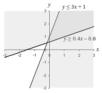
We can see in the graph that there are two shaded regions corresponding to the solutions to each inequality. The lines are shaded because the inequalities are not strict (≥ and ≤ are used). The solution to the system of inequalities is the darker shaded region, which is the overlap of the two individual regions, and the portions of the lines (rays) that border the region. Symbolically, we can perhaps best express the solution in this case as
0.4 x – 0.6 ≤ y ≤ 3 x + 1
Solving systems of inequalities in three or more dimensions is possible, but it is much more complicated-graphing the solid regions that constitute the solutions is likewise tougher.
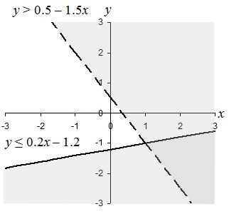
Practice Problem: Find and graph the solution set of the following system of inequalities:
x – 5 y ≥ 6
3 x + 2 y > 1
Solution : First, let's solve the expressions for y .
x – 5 y ≥ 6 3 x + 2 y > 1
x ≥ 6 + 5 y 2 y > 1 – 3 x
5 y ≤ x – 6 y > 0.5 – 1.5 x
y ≤ 0.2 x – 1.2
We can then express the solution to this system of inequalities as follows:
0.5 – 1.5 x < y ≤ 0.2 x – 1.2
Let's graph the solution set. First, we'll graph the lines corresponding to the two individual inequalities (and choosing a solid line for the first and a broken line for the second), then we'll shade the two regions appropriately.
Linear Optimization
We can apply what we have learned above to linear optimization (also called linear programming ), which is the process of finding a maximum or minimum value for some function under certain conditions (such as linear inequalities). Dealing with problems that involve linear optimization do not require you to learn any new skills; they simply require that you apply what you already know. So, let's move right to a practice problem.
Practice Problem: Find the maximum value of y given –3 x + 2 y ≤ 4 and x + y ≤ 1 subject to the condition that x ≥ 0.
Solution: What we are given is a system of inequalities for which we must first find a corresponding solution set. Within this solution set, we can then find the maximum value of y . So, we can first apply what we already know: let's rearrange the inequalities into a form that we can easily graph.
–3 x + 2 y ≤ 4 x + y ≤ 1 x ≥ 0
2 y ≤ 3 x + 4 y ≤ 1 – x
y ≤ 1.5 x + 2
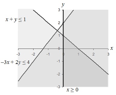
The darkest shaded region (the wedge in the lower right of the graph) satisfies all the constraints on the problem. We then want to find the maximum value of y , which is clearly 1. (We can also find this value by substituting x = 0 into x + y ≤ 1 and finding the maximum value of y , which likewise is clearly 1.)

- Course Catalog
- Group Discounts
- Gift Certificates
- For Libraries
- CEU Verification
- Medical Terminology
- Accounting Course
- Writing Basics
- QuickBooks Training
- Proofreading Class
- Sensitivity Training
- Excel Certificate
- Teach Online
- Terms of Service
- Privacy Policy


2.7 Solving Inequalities with Two Variables
Learning objectives.
- Identify and check solutions to inequalities with two variables.
- Graph solution sets of linear inequalities with two variables.
Solutions to Inequalities with Two Variables
We know that a linear equation with two variables has infinitely many ordered pair solutions that form a line when graphed. A linear inequality with two variables An inequality relating linear expressions with two variables. The solution set is a region defining half of the plane. , on the other hand, has a solution set consisting of a region that defines half of the plane.
For the inequality, the line defines the boundary of the region that is shaded. This indicates that any ordered pair in the shaded region, including the boundary line, will satisfy the inequality. To see that this is the case, choose a few test points A point not on the boundary of the linear inequality used as a means to determine in which half-plane the solutions lie. and substitute them into the inequality.
Also, we can see that ordered pairs outside the shaded region do not solve the linear inequality.
The graph of the solution set to a linear inequality is always a region. However, the boundary may not always be included in that set. In the previous example, the line was part of the solution set because of the “or equal to” part of the inclusive inequality ≤ . If given a strict inequality < , we would then use a dashed line to indicate that those points are not included in the solution set.
Consider the point (0, 3) on the boundary; this ordered pair satisfies the linear equation. It is the “or equal to” part of the inclusive inequality that makes the ordered pair part of the solution set.
So far we have seen examples of inequalities that were “less than.” Now consider the following graphs with the same boundary:
Given the graphs above, what might we expect if we use the origin (0, 0) as a test point?
Determine whether or not ( 2 , 1 2 ) is a solution to 5 x − 2 y < 10 .
Substitute the x - and y -values into the equation and see if a true statement is obtained.
5 x − 2 y < 10 5 ( 2 ) − 2 ( 1 2 ) < 10 10 − 1 < 10 9 < 10 ✓
Answer: ( 2 , 1 2 ) is a solution.
These ideas and techniques extend to nonlinear inequalities with two variables. For example, all of the solutions to y > x 2 are shaded in the graph below.

The boundary of the region is a parabola, shown as a dashed curve on the graph, and is not part of the solution set. However, from the graph we expect the ordered pair (−1,4) to be a solution. Furthermore, we expect that ordered pairs that are not in the shaded region, such as (−3, 2), will not satisfy the inequality.
Following are graphs of solutions sets of inequalities with inclusive parabolic boundaries.
You are encouraged to test points in and out of each solution set that is graphed above.
Try this! Is ( − 3 , − 2 ) a solution to 2 x − 3 y < 0 ?
Graphing Solutions to Inequalities with Two Variables
Solutions to linear inequalities are a shaded half-plane, bounded by a solid line or a dashed line. This boundary is either included in the solution or not, depending on the given inequality. If we are given a strict inequality, we use a dashed line to indicate that the boundary is not included. If we are given an inclusive inequality, we use a solid line to indicate that it is included. The steps for graphing the solution set for an inequality with two variables are shown in the following example.
Graph the solution set y > − 3 x + 1 .
Step 1: Graph the boundary. Because of the strict inequality, we will graph the boundary y = − 3 x + 1 using a dashed line. We can see that the slope is m = − 3 = − 3 1 = r i s e r u n and the y -intercept is (0, 1).

Step 2: Test a point that is not on the boundary. A common test point is the origin, (0, 0). The test point helps us determine which half of the plane to shade.
- Step 3: Shade the region containing the solutions. Since the test point (0, 0) was not a solution, it does not lie in the region containing all the ordered pair solutions. Therefore, shade the half of the plane that does not contain this test point. In this case, shade above the boundary line.

Consider the problem of shading above or below the boundary line when the inequality is in slope-intercept form. If y > m x + b , then shade above the line. If y < m x + b , then shade below the line. Shade with caution; sometimes the boundary is given in standard form, in which case these rules do not apply.
Graph the solution set 2 x − 5 y ≥ − 10 .
Here the boundary is defined by the line 2 x − 5 y = − 10 . Since the inequality is inclusive, we graph the boundary using a solid line. In this case, graph the boundary line using intercepts.

Next, test a point; this helps decide which region to shade.
Since the test point is in the solution set, shade the half of the plane that contains it.

In this example, notice that the solution set consists of all the ordered pairs below the boundary line. This may seem counterintuitive because the original inequality involved “greater than” ≥ . This illustrates that it is a best practice to actually test a point. Solve for y and you see that the shading is correct.
2 x − 5 y ≥ − 10 2 x − 5 y − 2 x ≥ − 10 − 2 x − 5 y ≥ − 2 x − 10 − 5 y − 5 ≤ − 2 x − 10 − 5 R e v e r s e t h e i n e q u a l i t y . y ≤ 2 5 x + 2
In slope-intercept form, you can see that the region below the boundary line should be shaded. An alternate approach is to first express the boundary in slope-intercept form, graph it, and then shade the appropriate region.
Graph the solution set y < 2 .
First, graph the boundary line y = 2 with a dashed line because of the strict inequality. Next, test a point.
In this case, shade the region that contains the test point.

Try this! Graph the solution set 2 x − 3 y < 0 .

The steps are the same for nonlinear inequalities with two variables. Graph the boundary first and then test a point to determine which region contains the solutions.
Graph the solution set y < ( x + 2 ) 2 − 1 .
The boundary is a basic parabola shifted 2 units to the left and 1 unit down. Begin by drawing a dashed parabolic boundary because of the strict inequality.

Next, test a point.
In this case, shade the region that contains the test point ( 0 , 0 ) .

Graph the solution set y ≥ x 2 + 3 .
The boundary is a basic parabola shifted 3 units up. It is graphed using a solid curve because of the inclusive inequality.

In this case, shade the region that does not contain the test point ( 0 , 0 ) .

Try this! Graph the solution set y < | x − 1 | − 3 .

Key Takeaways
- Linear inequalities with two variables have infinitely many ordered pair solutions, which can be graphed by shading in the appropriate half of a rectangular coordinate plane.
- To graph the solution set of an inequality with two variables, first graph the boundary with a dashed or solid line depending on the inequality. If given a strict inequality, use a dashed line for the boundary. If given an inclusive inequality, use a solid line. Next, choose a test point not on the boundary. If the test point solves the inequality, then shade the region that contains it; otherwise, shade the opposite side.
- Check your answer by testing points in and out of the shading region to verify that they solve the inequality or not.
Topic Exercises
Part a: solutions to inequalities with two variables.
Is the ordered pair a solution to the given inequality?
5 x − y > − 2 ; ( − 3 , − 4 )
4 x − y < − 8 ; ( − 3 , − 10 )
- 6 x − 15 y ≥ − 1 ; ( 1 2 , − 1 3 )
- x − 2 y ≥ 2 ; ( 2 3 , − 5 6 )
- 3 4 x − 2 3 y < 3 2 ; ( 1 , − 1 )
- 2 5 x + 4 3 y > 1 2 ; ( − 2 , 1 )
y ≤ x 2 − 1 ; ( − 1 , 1 )
y ≥ x 2 + 3 ; ( − 2 , 0 )
y ≥ ( x − 5 ) 2 + 1 ; ( 3 , 4 )
y ≤ 2 ( x + 1 ) 2 − 3 ; ( − 1 , − 2 )
y > 3 − | x | ; ( − 4 , − 3 )
y < | x | − 8 ; ( 5 , − 7 )
y > | 2 x − 1 | − 3 ; ( − 1 , 3 )
y < | 3 x − 2 | + 2 ; ( − 2 , 10 )
Part B: Graphing Solutions to Inequalities with Two Variables.
Graph the solution set.
y < 2 x − 1
y > − 4 x + 1
y ≥ − 2 3 x + 3
y ≤ 4 3 x − 3
2 x + 3 y ≤ 18
5 x + 2 y ≤ 8
6 x − 5 y > 30
8 x − 6 y < 24
3 x − 4 y < 0
x − 3 y > 0
- 1 6 x + 1 10 y ≤ 1 2
- 3 8 x + 1 2 y ≥ 3 4
- 1 12 x − 1 6 y < 2 3
- 1 3 x − 1 9 y > 4 3
5 x ≤ − 4 y − 12
− 4 x ≤ 12 − 3 y
4 y + 2 < 3 x
8 x < 9 − 6 y
5 ≥ 3 x − 15 y
- 2 x ≥ 6 − 9 y
Write an inequality that describes all points in the upper half-plane above the x -axis.
Write an inequality that describes all points in the lower half-plane below the x -axis.
Write an inequality that describes all points in the half-plane left of the y -axis.
Write an inequality that describes all points in the half-plane right of the y -axis.
Write an inequality that describes all ordered pairs whose y -coordinate is at least k units.
Write an inequality that describes all ordered pairs whose x -coordinate is at most k units.
y ≤ x 2 + 3
y > x 2 − 2
y > ( x + 1 ) 2
y > ( x − 2 ) 2
y ≤ ( x − 1 ) 2 + 2
y ≤ ( x + 3 ) 2 − 1
y < − x 2 + 1
y > − ( x − 2 ) 2 + 1
y ≥ | x | − 2
y < | x | + 1
y < | x − 3 |
y ≤ | x + 2 |
y > − | x + 1 |
y ≤ − | x − 2 |
y ≥ | x + 3 | − 2
y ≥ | x − 2 | − 1
y < − | x + 4 | + 2
y > − | x − 4 | − 1
y > x 3 − 1
y ≤ x 3 + 2
y > x − 1
A rectangular pen is to be constructed with at most 200 feet of fencing. Write a linear inequality in terms of the length l and the width w . Sketch the graph of all possible solutions to this problem.
A company sells one product for $8 and another for $12. How many of each product must be sold so that revenues are at least $2,400? Let x represent the number of products sold at $8 and let y represent the number of products sold at $12. Write a linear inequality in terms of x and y and sketch the graph of all possible solutions.

l + w ≤ 100 ;

Grade 8 Mathematics Module: “Solving Systems of Linear Inequalities in Two Variables”
This Self-Learning Module (SLM) is prepared so that you, our dear learners, can continue your studies and learn while at home. Activities, questions, directions, exercises, and discussions are carefully stated for you to understand each lesson.
Each SLM is composed of different parts. Each part shall guide you step-by-step as you discover and understand the lesson prepared for you.
Pre-tests are provided to measure your prior knowledge on lessons in each SLM. This will tell you if you need to proceed on completing this module or if you need to ask your facilitator or your teacher’s assistance for better understanding of the lesson. At the end of each module, you need to answer the post-test to self-check your learning. Answer keys are provided for each activity and test. We trust that you will be honest in using these.
Please use this module with care. Do not put unnecessary marks on any part of this SLM. Use a separate sheet of paper in answering the exercises and tests. And read the instructions carefully before performing each task.
If you have any questions in using this SLM or any difficulty in answering the tasks in this module, do not hesitate to consult your teacher or facilitator.
In this module, you will be acquainted with the application of systems of linear inequalities in two variables in solving problems related to real-life. The scope of this module enables you to use it in many different learning situations. The lesson is arranged following the standard sequence of the course. But the order in which you read them can be changed corresponding with the textbook you are now using.
This module is divided into two lessons:
- Lesson 1- Graphing Systems of Linear Inequalities in Two Variables
- Lesson 2– Solving Problems Involving Systems of Linear Inequalities in Two Variables
After going through this module, you are expected to:
1. define systems of linear inequalities in two variables;
2. graph systems of linear inequalities in two variables; and
3. solve problems involving systems of linear inequalities in two variables.
Grade 8 Mathematics Quarter 2 Self-Learning Module: “Solving Systems of Linear Inequalities in Two Variables”
Can't find what you're looking for.
We are here to help - please use the search box below.
Leave a Comment Cancel reply
If you're seeing this message, it means we're having trouble loading external resources on our website.
If you're behind a web filter, please make sure that the domains *.kastatic.org and *.kasandbox.org are unblocked.
To log in and use all the features of Khan Academy, please enable JavaScript in your browser.
Course: Algebra 1 > Unit 7
- Writing two-variable inequalities word problem
- Solving two-variable inequalities word problem
- Interpreting two-variable inequalities word problem
- Two-variable inequalities word problems
- Modeling with systems of inequalities
- Writing systems of inequalities word problem
- Solving systems of inequalities word problem
- Graphs of systems of inequalities word problem
- Systems of inequalities word problems
Graphs of two-variable inequalities word problem
- Inequalities (systems & graphs): FAQ
- Creativity break: What can we do to expand our creative skills?
Want to join the conversation?
- Upvote Button navigates to signup page
- Downvote Button navigates to signup page
- Flag Button navigates to signup page

Video transcript
Module 3: Quadratic Equations and Functions
Linear inequalities and systems of linear inequalities in two variables, learning objectives.
- Identify and follow steps for graphing a linear inequality in two variables
- Identify whether an ordered pair is in the solution set of a linear inequality
- Graph a system of linear inequalities and define the solutions region
- Verify whether a point is a solution to a system of inequalities
- Identify when a system of inequalities has no solution
- Solve systems of linear inequalities by graphing the solution region
- Graph solutions to a system that contains a compound inequality
- Write and graph a system that models the quantity that must be sold to achieve a given amount of sales
- Write a system of inequalities that represents the profit region for a business
- Interpret the solutions to a system of cost/ revenue inequalities
Inequalities in two variables
Did you know that you use linear inequalities when you shop online? When you use the option to view items within a specific price range, you are asking the search engine to use a linear inequality based on price. Essentially, you are saying “show me all the items for sale between $50 and $100,” which can be written as [latex]{50}\le {x} \le {100}[/latex], where x is price. In this section, you will apply what you know about graphing linear equations to graphing linear inequalities.
So how do you get from the algebraic form of an inequality, like [latex]y>3x+1[/latex], to a graph of that inequality? Plotting inequalities is fairly straightforward if you follow a couple steps.
Graphing Inequalities
To graph an inequality:
- Graph the related boundary line. Replace the <, >, ≤ or ≥ sign in the inequality with = to find the equation of the boundary line.
- Identify at least one ordered pair on either side of the boundary line and substitute those [latex](x,y)[/latex] values into the inequality. Shade the region that contains the ordered pairs that make the inequality a true statement.
- If points on the boundary line are solutions, then use a solid line for drawing the boundary line. This will happen for ≤ or ≥ inequalities.
- If points on the boundary line aren’t solutions, then use a dotted line for the boundary line. This will happen for < or > inequalities.
Let’s graph the inequality [latex]x+4y\leq4[/latex].
To graph the boundary line, find at least two values that lie on the line [latex]x+4y=4[/latex]. You can use the x – and y -intercepts for this equation by substituting 0 in for x first and finding the value of y ; then substitute 0 in for y and find x .
Plot the points [latex](0,1)[/latex] and [latex](4,0)[/latex], and draw a line through these two points for the boundary line. The line is solid because ≤ means “less than or equal to,” so all ordered pairs along the line are included in the solution set.

The next step is to find the region that contains the solutions. Is it above or below the boundary line? To identify the region where the inequality holds true, you can test a couple of ordered pairs, one on each side of the boundary line.
If you substitute [latex](−1,3)[/latex] into [latex]x+4y\leq4[/latex]:
[latex]\begin{array}{r}−1+4\left(3\right)\leq4\\−1+12\leq4\\11\leq4\end{array}[/latex]
This is a false statement, since 11 is not less than or equal to 4.
On the other hand, if you substitute [latex](2,0)[/latex] into [latex]x+4y\leq4[/latex]:
[latex]\begin{array}{r}2+4\left(0\right)\leq4\\2+0\leq4\\2\leq4\end{array}[/latex]
This is true! The region that includes [latex](2,0)[/latex] should be shaded, as this is the region of solutions.

And there you have it—the graph of the set of solutions for [latex]x+4y\leq4[/latex].
Graphing Linear Inequalities in Two Variables
Graph the inequality [latex]2y>4x–6[/latex].
Solve for y .
[latex] \displaystyle \begin{array}{r}2y>4x-6\\\\\frac{2y}{2}>\frac{4x}{2}-\frac{6}{2}\\\\y>2x-3\\\end{array}[/latex]
Create a table of values to find two points on the line [latex] \displaystyle y=2x-3[/latex], or graph it based on the slope-intercept method, the b value of the y -intercept is [latex]-3[/latex] and the slope is 2.
Plot the points, and graph the line. The line is dotted because the sign in the inequality is >, not ≥ and therefore points on the line are not solutions to the inequality.

[latex] \displaystyle y=2x-3[/latex]
Find an ordered pair on either side of the boundary line. Insert the x – and y -values into the inequality [latex]2y>4x–6[/latex] and see which ordered pair results in a true statement. Since [latex](−3,1)[/latex] results in a true statement, the region that includes [latex](−3,1)[/latex] should be shaded.
[latex]\begin{array}{l}2y>4x–6\\\\\text{Test }1:\left(−3,1\right)\\2\left(1\right)>4\left(−3\right)–6\\\,\,\,\,\,\,\,2>–12–6\\\,\,\,\,\,\,\,2>−18\\\text{TRUE}\\\\\text{Test }2:\left(4,1\right)\\2(1)>4\left(4\right)– 6\\\,\,\,\,\,\,2>16–6\\\,\,\,\,\,\,2>10\\\text{FALSE}\end{array}[/latex]
The graph of the inequality [latex]2y>4x–6[/latex] is:

A quick note about the problem above—notice that you can use the points [latex](0,−3)[/latex] and [latex](2,1)[/latex] to graph the boundary line, but that these points are not included in the region of solutions, since the region does not include the boundary line!
Solution Sets of Inequalities
The graph below shows the region of values that makes the inequality [latex]3x+2y\leq6[/latex] true (shaded red), the boundary line [latex]3x+2y=6[/latex], as well as a handful of ordered pairs. The boundary line is solid because points on the boundary line [latex]3x+2y=6[/latex] will make the inequality [latex]3x+2y\leq6[/latex] true.

You can substitute the x- and y- values in each of the [latex](x,y)[/latex] ordered pairs into the inequality to find solutions. Sometimes making a table of values makes sense for more complicated inequalities.
If substituting [latex](x,y)[/latex] into the inequality yields a true statement, then the ordered pair is a solution to the inequality, and the point will be plotted within the shaded region or the point will be part of a solid boundary line. A false statement means that the ordered pair is not a solution, and the point will graph outside the shaded region, or the point will be part of a dotted boundary line.
Use the graph to determine which ordered pairs plotted below are solutions of the inequality [latex]x–y<3[/latex].

Solutions will be located in the shaded region. Since this is a “less than” problem, ordered pairs on the boundary line are not included in the solution set.
These values are located in the shaded region, so are solutions. (When substituted into the inequality [latex]x–y<3[/latex], they produce true statements.)
[latex](−1,1)[/latex]
[latex](−2,−2)[/latex]
These values are not located in the shaded region, so are not solutions. (When substituted into the inequality [latex]x-y<3[/latex], they produce false statements.)
[latex](1,−2)[/latex]
[latex](3,−2)[/latex]
[latex](4,0)[/latex]
[latex](−1,1)\,\,\,(−2,−2)[/latex]
The following video show an example of determining whether an ordered pair is a solution to an inequality.
Is [latex](2,−3)[/latex] a solution of the inequality [latex]y<−3x+1[/latex]?
If [latex](2,−3)[/latex] is a solution, then it will yield a true statement when substituted into the inequality [latex]y<−3x+1[/latex].
[latex]y<−3x+1[/latex]
Substitute [latex]x=2[/latex] and [latex]y=−3[/latex] into inequality.
[latex]−3<−3\left(2\right)+1[/latex]
[latex]\begin{array}{l}−3<−6+1\\−3<−5\end{array}[/latex]
This statement is not true, so the ordered pair [latex](2,−3)[/latex] is not a solution.
[latex](2,−3)[/latex] is not a solution.
The following video shows another example of determining whether an ordered pair is a solution to an inequality.
Graph a system of two inequalities
Consider the graph of the inequality [latex]y<2x+5[/latex].
The dashed line is [latex]y=2x+5[/latex]. Every ordered pair in the shaded area below the line is a solution to [latex]y<2x+5[/latex], as all of the points below the line will make the inequality true. If you doubt that, try substituting the x and y coordinates of Points A and B into the inequality—you’ll see that they work. So, the shaded area shows all of the solutions for this inequality.
The boundary line divides the coordinate plane in half. In this case, it is shown as a dashed line as the points on the line don’t satisfy the inequality. If the inequality had been [latex]y\leq2x+5[/latex], then the boundary line would have been solid.
Let’s graph another inequality: [latex]y>−x[/latex]. You can check a couple of points to determine which side of the boundary line to shade. Checking points M and N yield true statements. So, we shade the area above the line. The line is dashed as points on the line are not true.
To create a system of inequalities, you need to graph two or more inequalities together. Let’s use [latex]y<2x+5[/latex] and [latex]y>−x[/latex] since we have already graphed each of them.
The purple area shows where the solutions of the two inequalities overlap. This area is the solution to the system of inequalities . Any point within this purple region will be true for both [latex]y>−x[/latex] and [latex]y<2x+5[/latex].
In the following video examples, we show how to graph a system of linear inequalities, and define the solution region.
In the next section, we will see that points can be solutions to systems of equations and inequalities. We will verify algebraically whether a point is a solution to a linear equation or inequality.
Determine whether an ordered pair is a solution to a system of linear inequalities
On the graph above, you can see that the points B and N are solutions for the system because their coordinates will make both inequalities true statements.
In contrast, points M and A both lie outside the solution region (purple). While point M is a solution for the inequality [latex]y>−x[/latex] and point A is a solution for the inequality [latex]y<2x+5[/latex], neither point is a solution for the system . The following example shows how to test a point to see whether it is a solution to a system of inequalities.
Is the point (2, 1) a solution of the system [latex]x+y>1[/latex] and [latex]2x+y<8[/latex]?
[latex]\begin{array}{r}x+y>1\\2+1>1\\3>1\\\text{TRUE}\end{array}[/latex]
(2, 1) is a solution for [latex]x+y>1[/latex].
[latex]\begin{array}{r}2x+y<8\\2\left(2\right)+1<8\\4+1<8\\5<8\\\text{TRUE}\end{array}[/latex]
(2, 1) is a solution for [latex]2x+y<8.[/latex]
Since (2, 1) is a solution of each inequality, it is also a solution of the system.
The point (2, 1) is a solution of the system [latex]x+y>1[/latex] and [latex]2x+y<8[/latex].
Here is a graph of the system in the example above. Notice that (2, 1) lies in the purple area, which is the overlapping area for the two inequalities.
Is the point (2, 1) a solution of the system [latex]x+y>1[/latex] and [latex]3x+y<4[/latex]?
Check the point with each of the inequalities. Substitute 2 for x and 1 for y . Is the point a solution of both inequalities?
[latex]\begin{array}{r}3x+y<4\\3\left(2\right)+1<4\\6+1<4\\7<4\\\text{FALSE}\end{array}[/latex]
(2, 1) is not a solution for [latex]3x+y<4[/latex].
Since (2, 1) is not a solution of one of the inequalities, it is not a solution of the system.
The point (2, 1) is not a solution of the system [latex]x+y>1[/latex] and [latex]3x+y<4[/latex].
Here is a graph of this system. Notice that (2, 1) is not in the purple area, which is the overlapping area; it is a solution for one inequality (the red region), but it is not a solution for the second inequality (the blue region).
In the following video we show another example of determining whether a point is in the solution of a system of linear inequalities.
As shown above, finding the solutions of a system of inequalities can be done by graphing each inequality and identifying the region they share. Below, you are given more examples that show the entire process of defining the region of solutions on a graph for a system of two linear inequalities. The general steps are outlined below:
- Graph each inequality as a line and determine whether it will be solid or dashed
- Determine which side of each boundary line represents solutions to the inequality by testing a point on each side
- Shade the region that represents solutions for both inequalities
Systems with no solutions
In the next example, we will show the solution to a system of two inequalities whose boundary lines are parallel to each other. When the graphs of a system of two linear equations are parallel to each other, we found that there was no solution to the system. We will get a similar result for the following system of linear inequalities.
Graph the system [latex]\begin{array}{c}y\ge2x+1\\y\lt2x-3\end{array}[/latex]
The boundary lines for this system are parallel to each other, note how they have the same slopes.
[latex]\begin{array}{c}y=2x+1\\y=2x-3\end{array}[/latex]
Plotting the boundary lines will give the graph below. Note that the inequality [latex]y\lt2x-3[/latex] requires that we draw a dashed line, while the inequality [latex]y\ge2x+1[/latex] will require a solid line.

Now we need to add the regions that represent the inequalities. For the inequality [latex]y\ge2x+1[/latex] we can test a point on either side of the line to see which region to shade. Let’s test [latex]\left(0,0\right)[/latex] to make it easy.
Substitute [latex]\left(0,0\right)[/latex] into [latex]y\ge2x+1[/latex]
[latex]\begin{array}{c}y\ge2x+1\\0\ge2\left(0\right)+1\\0\ge{1}\end{array}[/latex]
This is not true, so we know that we need to shade the other side of the boundary line for the inequality [latex]y\ge2x+1[/latex]. The graph will now look like this:

Now let’s shade the region that shows the solutions to the inequality [latex]y\lt2x-3[/latex]. Again, we can pick [latex]\left(0,0\right)[/latex] to test because it makes easy algebra.
Substitute [latex]\left(0,0\right)[/latex] into [latex]y\lt2x-3[/latex]
[latex]\begin{array}{c}y\lt2x-3\\0\lt2\left(0,\right)x-3\\0\lt{-3}\end{array}[/latex]
This is not true, so we know that we need to shade the other side of the boundary line for the inequality[latex]y\lt2x-3[/latex]. The graph will now look like this:

This system of inequalities shares no points in common.
In the following examples, we will continue to practice graphing the solution region for systems of linear inequalities. We will also graph the solutions to a system that includes a compound inequality.
Shade the region of the graph that represents solutions for both inequalities. [latex]x+y\geq1[/latex] and [latex]y–x\geq5[/latex].

Find an ordered pair on either side of the boundary line. Insert the x – and y -values into the inequality [latex]x+y\geq1[/latex] and see which ordered pair results in a true statement.
[latex]\begin{array}{r}\text{Test }1:\left(−3,0\right)\\x+y\geq1\\−3+0\geq1\\−3\geq1\\\text{FALSE}\\\\\text{Test }2:\left(4,1\right)\\x+y\geq1\\4+1\geq1\\5\geq1\\\text{TRUE}\end{array}[/latex]
Since (4, 1) results in a true statement, the region that includes (4, 1) should be shaded.
Do the same with the second inequality. Graph the boundary line, then test points to find which region is the solution to the inequality. In this case, the boundary line is [latex]y–x=5\left(\text{or }y=x+5\right)[/latex] and is solid. Test point (−3, 0) is not a solution of [latex]y–x\geq5[/latex], and test point (0, 6) is a solution.
The purple region in this graph shows the set of all solutions of the system.

The videos that follow show more examples of graphing the solution set of a system of linear inequalities.
The system in our last example includes a compound inequality. We will see that you can treat a compound inequality like two lines when you are graphing them.
Find the solution to the system 3 x + 2 y < 12 and −1 ≤ y ≤ 5.
Graph one inequality. First graph the boundary line, then test points.
Remember, because the inequality 3 x + 2 y < 12 does not include the equal sign, draw a dashed border line.
Testing a point (like (0, 0) will show that the area below the line is the solution to this inequality.
The inequality −1 ≤ y ≤ 5 is actually two inequalities: −1 ≤ y , and y ≤ 5. Another way to think of this is y must be between −1 and 5. The border lines for both are horizontal. The region between those two lines contains the solutions of −1 ≤ y ≤ 5. We make the lines solid because we also want to include y = −1 and y = 5.
Graph this region on the same axes as the other inequality.

In the video that follows, we show how to solve another system of inequalities.
Applications
In our first example we will show how to write and graph a system of linear inequalities that models the amount of sales needed to obtain a specific amount of money.
Cathy is selling ice cream cones at a school fundraiser. She is selling two sizes: small (which has 1 scoop) and large (which has 2 scoops). She knows that she can get a maximum of 70 scoops of ice cream out of her supply. She charges $3 for a small cone and $5 for a large cone.
Cathy wants to earn at least $120 to give back to the school. Write and graph a system of inequalities that models this situation.
First, identify the variables. There are two variables: the number of small cones and the number of large cones.
s = small cone
l = large cone
Write the first equation: the maximum number of scoops she can give out. The scoops she has available (70) must be greater than or equal to the number of scoops for the small cones ( s ) and the large cones (2 l ) she sells.
[latex]s+2l\le70[/latex]
Write the second equation: the amount of money she raises. She wants the total amount of money earned from small cones (3 s ) and large cones (5 l ) to be at least $120.
[latex]3s+5l\ge120[/latex]
Write the system.
[latex]\begin{cases}s+2l\le70\\3s+5l\ge120\end{cases}[/latex]
Now graph the system. The variables x and y have been replaced by s and l ; graph s along the x -axis, and l along the y -axis.

Now graph the region [latex]3s+5l\ge120[/latex] Graph the boundary line and then test individual points to see which region to shade. The graph is shown below.

Graphing the regions together, you find the following:

The region in purple is the solution. As long as the combination of small cones and large cones that Cathy sells can be mapped in the purple region, she will have earned at least $120 and not used more than 70 scoops of ice cream.
In a previous example for finding a solution to a system of linear equations, we introduced a manufacturer’s cost and revenue equations:
Cost: [latex]y=0.85x+35,000[/latex]
Revenue: [latex]y=1.55x[/latex]
The cost equation is shown in blue in the graph below, and the revenue equation is graphed in orange.The point at which the two lines intersect is called the break-even point, we learned that this is the solution to the system of linear equations that in this case comprise the cost and revenue equations.
The shaded region to the right of the break-even point represents quantities for which the company makes a profit. The region to the left represents quantities for which the company suffers a loss.
In the next example, you will see how the information you learned about systems of linear inequalities can be applied to answering questions about cost and revenue.

Note how the blue shaded region between the Cost and Revenue equations is labeled Profit. This is the “sweet spot” that the company wants to achieve where they produce enough bike frames at a minimal enough cost to make money. They don’t want more money going out than coming in!
Define the profit region for the skateboard manufacturing business using inequalities, given the system of linear equations:
We know that graphically, solutions to linear inequalities are entire regions, and we learned how to graph systems of linear inequalities earlier in this module. Based on the graph below and the equations that define cost and revenue, we can use inequalities to define the region for which the skateboard manufacturer will make a profit.

Let’s start with the revenue equation. We know that the break even point is at (50,000, 77,500) and the profit region is the blue area. If we choose a point in the region and test it like we did for finding solution regions to inequalities, we will know which kind of inequality sign to use.
Let’s test the point [latex]\left(65,00,100,000\right)[/latex] in both equations to determine which inequality sign to use.
[latex]\begin{array}{l}y=0.85x+{35,000}\\{100,000}\text{ ? }0.85\left(65,000\right)+35,000\\100,000\text{ ? }90,250\end{array}[/latex]
We need to use > because 100,000 is greater than 90,250
The cost inequality that will ensure the company makes profit – not just break even – is [latex]y>0.85x+35,000[/latex]
Now test the point in the revenue equation:
[latex]\begin{array}{l}y=1.55x\\100,000\text{ ? }1.55\left(65,000\right)\\100,000\text{ ? }100,750\end{array}[/latex]
We need to use < because 100,000 is less than 100,750
The revenue inequality that will ensure the company makes profit – not just break even – is [latex]y<1.55x[/latex]
The systems of inequalities that defines the profit region for the bike manufacturer:
[latex]\begin{array}{l}y>0.85x+35,000\\y<1.55x\end{array}[/latex]
The cost to produce 50,000 units is $77,500, and the revenue from the sales of 50,000 units is also $77,500. To make a profit, the business must produce and sell more than 50,000 units. The system of linear inequalities that represents the number of units that the company must produce in order to earn a profit is:
In the following video you will see an example of how to find the break even point for a small sno-cone business.
And here is one more video example of solving an application using a sustem of linear inequalities.
We have seen that systems of linear equations and inequalities can help to define market behaviors that are very helpful to businesses. The intersection of cost and revenue equations gives the break even point, and also helps define the region for which a company will make a profit.
- Ex 1: Graphing Linear Inequalities in Two Variables (Slope Intercept Form). Authored by : James Sousa (Mathispower4u.com) . Located at : https://youtu.be/Hzxc4HASygU . License : CC BY: Attribution
- System of Equations App: Break-Even Point.. Authored by : James Sousa (Mathispower4u.com) for Lumen Learning. Located at : . License : CC BY: Attribution
- Revision and Adaptation. Provided by : Lumen Learning. License : CC BY: Attribution
- Ex 2: Graphing Linear Inequalities in Two Variables (Standard Form). Authored by : James Sousa (Mathispower4u.com) . Located at : https://youtu.be/2VgFg2ztspI . License : CC BY: Attribution
- Unit 13: Graphing, from Developmental Math: An Open Program. Provided by : Monterey Institute of Technology and Education. Located at : http://nrocnetwork.org/dm-opentext . License : CC BY: Attribution
- Use a Graph Determine Ordered Pair Solutions of a Linear Inequalty in Two Variable. Authored by : James Sousa (Mathispower4u.com) for Lumen Learning. Located at : https://youtu.be/GQVdDRVq5_o . License : CC BY: Attribution
- Ex: Determine if Ordered Pairs Satisfy a Linear Inequality. Authored by : James Sousa (Mathispower4u.com) . Located at : https://youtu.be/-x-zt_yM0RM . License : CC BY: Attribution
- Ex 1: Graph a System of Linear Inequalities. . Authored by : James Sousa (Mathispower4u.com) .. Located at : . License : CC BY: Attribution
- Ex 2: Graph a System of Linear Inequalities.. Authored by : James Sousa (Mathispower4u.com). Located at : . License : CC BY: Attribution
- Unit 14: Systems of Equations and Inequalities, from Developmental Math: An Open Program.. Provided by : Monterey Institute of Technology. . Located at : http://nrocnetwork.org/dm-opentext. . License : CC BY: Attribution
- Determine the Solution to a System of Inequalities (Compound).. Authored by : James Sousa (Mathispower4u.com) . Located at : . License : CC BY: Attribution
- College Algebra. Authored by : Jay Abrams, et al.. Provided by : OpenStax. Located at : https://openstaxcollege.org/textbooks/college-algebra. . License : CC BY: Attribution

Privacy Policy

- school Campus Bookshelves
- menu_book Bookshelves
- perm_media Learning Objects
- login Login
- how_to_reg Request Instructor Account
- hub Instructor Commons
Margin Size
- Download Page (PDF)
- Download Full Book (PDF)
- Periodic Table
- Physics Constants
- Scientific Calculator
- Reference & Cite
- Tools expand_more
- Readability
selected template will load here
This action is not available.
3.8: Linear Inequalities (Two Variables)
- Last updated
- Save as PDF
- Page ID 24123
\( \newcommand{\vecs}[1]{\overset { \scriptstyle \rightharpoonup} {\mathbf{#1}} } \)
\( \newcommand{\vecd}[1]{\overset{-\!-\!\rightharpoonup}{\vphantom{a}\smash {#1}}} \)
\( \newcommand{\id}{\mathrm{id}}\) \( \newcommand{\Span}{\mathrm{span}}\)
( \newcommand{\kernel}{\mathrm{null}\,}\) \( \newcommand{\range}{\mathrm{range}\,}\)
\( \newcommand{\RealPart}{\mathrm{Re}}\) \( \newcommand{\ImaginaryPart}{\mathrm{Im}}\)
\( \newcommand{\Argument}{\mathrm{Arg}}\) \( \newcommand{\norm}[1]{\| #1 \|}\)
\( \newcommand{\inner}[2]{\langle #1, #2 \rangle}\)
\( \newcommand{\Span}{\mathrm{span}}\)
\( \newcommand{\id}{\mathrm{id}}\)
\( \newcommand{\kernel}{\mathrm{null}\,}\)
\( \newcommand{\range}{\mathrm{range}\,}\)
\( \newcommand{\RealPart}{\mathrm{Re}}\)
\( \newcommand{\ImaginaryPart}{\mathrm{Im}}\)
\( \newcommand{\Argument}{\mathrm{Arg}}\)
\( \newcommand{\norm}[1]{\| #1 \|}\)
\( \newcommand{\Span}{\mathrm{span}}\) \( \newcommand{\AA}{\unicode[.8,0]{x212B}}\)
\( \newcommand{\vectorA}[1]{\vec{#1}} % arrow\)
\( \newcommand{\vectorAt}[1]{\vec{\text{#1}}} % arrow\)
\( \newcommand{\vectorB}[1]{\overset { \scriptstyle \rightharpoonup} {\mathbf{#1}} } \)
\( \newcommand{\vectorC}[1]{\textbf{#1}} \)
\( \newcommand{\vectorD}[1]{\overrightarrow{#1}} \)
\( \newcommand{\vectorDt}[1]{\overrightarrow{\text{#1}}} \)
\( \newcommand{\vectE}[1]{\overset{-\!-\!\rightharpoonup}{\vphantom{a}\smash{\mathbf {#1}}}} \)
Learning Objectives
- Identify and check solutions to linear inequalities with two variables.
- Graph solution sets of linear inequalities with two variables.
Solutions to Linear Inequalities
We know that a linear equation with two variables has infinitely many ordered pair solutions that form a line when graphed. A linear inequality with two variables, on the other hand, has a solution set consisting of a region that defines half of the plane.
For the inequality, the line defines one boundary of the region that is shaded. This indicates that any ordered pair that is in the shaded region, including the boundary line, will satisfy the inequality. To see that this is the case, choose a few test points and substitute them into the inequality.
Also, we can see that ordered pairs outside the shaded region do not solve the linear inequality.
\(\begin{array} {c|c} {\underline{\color{Cerulean}{Test\:point}}}&{\underline{y\leq\frac{3}{2}x+3}}\\{(-2,3)} &{3\leq\frac{3}{2}(-2)+3}\\{}&{3\leq -3+3}\\{}&{3\leq 0\quad\color{red}{x}} \end{array}\)
The graph of the solution set to a linear inequality is always a region. However, the boundary may not always be included in that set. In the previous example, the line was part of the solution set because of the “or equal to” part of the inclusive inequality \(≤\). If we have a strict inequality \(<\), we would then use a dashed line to indicate that those points are not included in the solution set.
Consider the point \((0, 3)\) on the boundary; this ordered pair satisfies the linear equation. It is the “or equal to” part of the inclusive inequality that makes it part of the solution set.
\(\begin{array}{c|c}{\underline{y<\frac{3}{2}x+3}}&{\underline{y\leq \frac{3}{2}x+3}}\\{3<\frac{3}{2}(0)+3}&{3\leq\frac{3}{2}(0)+3}\\{3<0+3}&{3\leq 0+3}\\{3<3\quad\color{red}{x}}&{3\leq 3\quad\color{Cerulean}{\checkmark}} \end{array}\)
So far, we have seen examples of inequalities that were “less than.” Now consider the following graphs with the same boundary:
Given the graphs above, what might we expect if we use the origin \((0, 0)\) as a test point?
\(\begin{array}{c|c}{\underline{y\geq\frac{3}{2}x+3}}&{\underline{y\leq\frac{3}{2}x+3}}\\{0\geq\frac{3}{2}(0)+3}&{0\leq\frac{3}{2}(0)+3}\\{0\geq 0+3}&{0\leq0+3}\\{0\geq 3\quad\color{red}{x}}&{0\leq 3\quad\color{Cerulean}{\checkmark}} \end{array}\)
Exercise \(\PageIndex{1}\)
Which of the ordered pairs \((−2, −1), (0, 0), (−2, 8), (2, 1),\) and \((4, 2)\) solve the inequality \(y>−\frac{1}{2}x+2\)?
\((−2, 8)\) and \((4, 2)\)
Graphing Solutions to Linear Inequalities
Solutions to linear inequalities are a shaded half-plane, bounded by a solid line or a dashed line. This boundary is either included in the solution or not, depending on the given inequality. If we are given a strict inequality, we use a dashed line to indicate that the boundary is not included. If we are given an inclusive inequality, we use a solid line to indicate that it is included. The steps for graphing the solution set for an inequality with two variables are outlined in the following example.
Example \(\PageIndex{1}\)
Graph the solution set:
\(y>−3x+1\).
Step 1 : Graph the boundary line. In this case, graph a dashed line \(y=−3x+1\) because of the strict inequality. By inspection, we see that the slope is \(m=−3=−\frac{3}{1}=\frac{rise}{run}\) and the \(y\)-intercept is \((0, 1)\).
.png?revision=1 "problem solving involving system of linear inequalities in two variables")
Figure \(\PageIndex{7}\)
Step 2 : Test a point not on the boundary. A common test point is the origin \((0, 0)\). The test point helps us determine which half of the plane to shade.
\(\begin{array}{c|c} {\underline{\color{Cerulean}{Test\:point}}}&{\underline{y>-3x+1}}\\{(0,0)}&{0>-3(0)+1}\\{}&{0>1\quad\color{red}{x}} \end{array}\)
Step 3 : Shade the region containing the solutions. Since the test point \((0, 0)\) was not a solution, it does not lie in the region containing all the ordered pair solutions. Therefore, shade the half of the plane that does not contain this test point. In this case, shade above the boundary line.
.png?revision=1 "problem solving involving system of linear inequalities in two variables")
Figure \(\PageIndex{8}\)
Consider the problem of shading above or below the boundary line when the inequality is in slope-intercept form. If \(y>mx+b\), then shade above the line. If \(y<mx+b\), then shade below the line. Use this with caution; sometimes the boundary is given in standard form, in which case these rules do not apply.
Example \(\PageIndex{2}\)
\(2x−5y≥−10\).
Here the boundary is defined by the line \(2x−5y=−10\). Since the inequality is inclusive, we graph the boundary using a solid line. In this case, graph the boundary line using intercepts.
.png?revision=1 "problem solving involving system of linear inequalities in two variables")
Figure \(\PageIndex{9}\)
Next, test a point; this helps decide which region to shade.
\(\begin{array} {c|c} {\underline{\color{Cerulean}{Test\:point}}}&{\underline{2x-5y\geq -10}}\\{(0,0)}&{2(0)-5(0)\geq -10} \\ {}&{0\geq -10\quad\color{Cerulean}{\checkmark}} \end{array}\)
Since the test point is in the solution set, shade the half of the plane that contains it.
.png?revision=1 "problem solving involving system of linear inequalities in two variables")
Figure \(\PageIndex{10}\)
In this example, notice that the solution set consists of all the ordered pairs below the boundary line. This may be counterintuitive because of the original \(≥\) in the inequality. This illustrates that it is a best practice to actually test a point. Solve for \(y\) and you see that the shading is correct.
In slope-intercept form, you can see that the region below the boundary line should be shaded. An alternate approach is to first express the boundary in slope-intercept form, graph it, and then shade the appropriate region.
Example \(\PageIndex{3}\)
\(y<2\).
First, graph the boundary line \(y=2\) with a dashed line because of the strict inequality.
.png?revision=1 "problem solving involving system of linear inequalities in two variables")
Figure \(\PageIndex{11}\)
Now, test a point.
\(\begin{array}{c|c}{\underline{\color{Cerulean}{Test\:point}}}&{\underline{y<2}}\\{(0,0)}&{0<2\quad\color{Cerulean}{\checkmark}} \end{array}\)
In this case, shade the region that contains the test point.
.png?revision=1 "problem solving involving system of linear inequalities in two variables")
Figure \(\PageIndex{12}\)
Exercise \(\PageIndex{2}\)
\(5x−y≤10\).
.png?revision=1 "problem solving involving system of linear inequalities in two variables")
Figure \(\PageIndex{13}\)
Key Takeaways
- Linear inequalities with two variables have infinitely many ordered pair solutions, which can be graphed by shading in the appropriate half of a rectangular coordinate plane.
- To graph the solution set of a linear inequality with two variables, first graph the boundary with a dashed or solid line depending on the inequality. If given a strict inequality, use a dashed line for the boundary. If given an inclusive inequality, use a solid line. Next, choose a test point not on the boundary. If the test point solves the inequality, then shade the region that contains it; otherwise, shade the opposite side.
- When graphing the solution sets of linear inequalities, it is a good practice to test values in and out of the solution set as a check.
Exercise \(\PageIndex{3}\) Solutions to Linear Inequalities (Two Variables)
Is the ordered pair a solution to the given inequality?
- \(y<5x+1\); \((0,0)\)
- \(y>−\frac{1}{2}x−4\); \((0, −2)\)
- \(y≤\frac{2}{3}x+1\); \((6, 5)\)
- \(y≥−\frac{1}{3}x−5\); \((−3, −8)\)
- \(y<\frac{1}{5}x-\frac{1}{3}\); \((-\frac{1}{2},-1)\)
- \(4x-3y\leq 2\); \((-2,-1)\)
- \(-x+4y>7\); \((0, 0)\)
- \(7x−3y<21\); \((5,-3)\)
- \(y>−5\); \((−3, −1)\)
- \(x≤0\); \((0, 7)\)
Exercise \(\PageIndex{4}\) Graphing Solutions to Linear Inequalities
Graph the solution set.
- \(y<−3x+3\)
- \(y<−\frac{2}{3}x+4\)
- \(y≥−\frac{1}{2}x\)
- \(y≥\frac{4}{5}x−8\)
- \(y≤8x−7\)
- \(y>−5x+3\)
- \(y>−x+4\)
- \(y>x−2\)
- \(y≥−1\)
- \(y<−3\)
- \(y≤\frac{3}{4}x−\frac{1}{2}\)
- \(y>−\frac{3}{2}x+\frac{5}{2}\)
- \(−2x+3y>6\)
- \(7x−2y>14\)
- \(5x−y<10\)
- \(x-y<0\)
- \(3x−2y≥0\)
- \(x−5y≤0\)
- \(−x+2y≤−4\)
- \(−x+2y≤3\)
- \(2x−3y≥−1\)
- \(5x−4y<−3\)
- \(\frac{1}{2}x-\frac{1}{3}y<1\)
- \(\frac{1}{2}x-\frac{1}{10}y\geq\frac{1}{2}\)
- \(x≥−2y\)
- \(x<2y+3\)
- \(3x−y+2>0\)
- \(3−y−2x<0\)
- \(−4x≤12−3y\)
- \(5x≤−4y−12\)
- Write an inequality that describes all points in the upper half-plane above the \(x\)-axis.
- Write an inequality that describes all points in the lower half-plane below the \(x\)-axis.
- Write an inequality that describes all points in the half-plane left of the \(y\)-axis.
- Write an inequality that describes all points in the half-plane right of the \(y\)-axis.
- Write an inequality that describes all ordered pairs whose \(y\)-coordinates are at least \(2\).
- Write an inequality that describes all ordered pairs whose \(x\)-coordinate is at most \(5\).
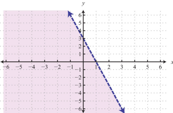.png?revision=1 "problem solving involving system of linear inequalities in two variables")
Figure \(\PageIndex{14}\)
.png?revision=1 "problem solving involving system of linear inequalities in two variables")
Figure \(\PageIndex{15}\)
.png?revision=1 "problem solving involving system of linear inequalities in two variables")
Figure \(\PageIndex{16}\)
.png?revision=1 "problem solving involving system of linear inequalities in two variables")
Figure \(\PageIndex{17}\)
.png?revision=1 "problem solving involving system of linear inequalities in two variables")
Figure \(\PageIndex{18}\)
.png?revision=1 "problem solving involving system of linear inequalities in two variables")
Figure \(\PageIndex{19}\)
.png?revision=1 "problem solving involving system of linear inequalities in two variables")
Figure \(\PageIndex{20}\)
.png?revision=1 "problem solving involving system of linear inequalities in two variables")
Figure \(\PageIndex{21}\)
.png?revision=1 "problem solving involving system of linear inequalities in two variables")
Figure \(\PageIndex{22}\)
.png?revision=1 "problem solving involving system of linear inequalities in two variables")
Figure \(\PageIndex{23}\)
.png?revision=1 "problem solving involving system of linear inequalities in two variables")
Figure \(\PageIndex{24}\)
.png?revision=1 "problem solving involving system of linear inequalities in two variables")
Figure \(\PageIndex{25}\)
.png?revision=1 "problem solving involving system of linear inequalities in two variables")
Figure \(\PageIndex{26}\)
.png?revision=1 "problem solving involving system of linear inequalities in two variables")
Figure \(\PageIndex{27}\)
.png?revision=1 "problem solving involving system of linear inequalities in two variables")
Figure \(\PageIndex{28}\)
.png?revision=1 "problem solving involving system of linear inequalities in two variables")
Figure \(\PageIndex{29}\)
33. \(y>0\)
35. \(x<0\)
37. \(y≥2\)
- Math Article
Linear Inequalities In Two Variables
Linear inequalities in two variables represent the inequalities between two algebraic expressions where two distinct variables are included. In linear inequalities in two variables, we use greater than (>), less than (<), greater than or equal (≥) and less than or equal (≤) symbols, instead of using equal to a symbol (=).
What is Linear Inequalities?
Any two real numbers or two algebraic expressions associated with the symbol ‘<’, ‘>’, ‘≤’ or ‘≥’ form a linear inequality. For example, 9<11, 18>17 are examples of numerical inequalities and x+7>y, y<10-x, x ≥ y > 11 are examples of algebraic inequalities.
The symbols ‘<‘ and ‘>’ represent the strict inequalities and the symbols ‘≤’ and ‘≥’ represent slack inequalities. To represent linear inequalities in one variable in a number line is a visual representation and is a convenient way to represent the solutions of the inequality. Now, we will discuss the graph of a linear inequality in two variables.
What are Linear Inequalities in Two Variables?
Linear inequalities in two variables represent the unequal relation between two algebraic expressions that includes two distinct variables. Hence, the symbols used between the expression in two variables will be ‘<’, ‘>’, ‘≤’ or ‘≥’, but we cannot use equal to ‘=’ symbol here.
The examples of linear inequalities in two variables are:
- 3x < 2y + 5
- 8y – 9x > 10
Note: 4x 2 + 2x + 5 < 0 is not an example of linear inequality in one variable, because the exponent of x is 2 in the first term. It is a quadratic inequality.
How to Solve Linear Inequalities in Two Variables?
The solution for linear inequalities in two variables is an ordered pair that is true for the inequality statement. Let us say if Ax + By > C is a linear inequality where x and y are two variables, then an ordered pair (x, y) satisfying the statement will be the required solution.
The method of solving linear inequalities in two variables is the same as solving linear equations .
For example, if 2x + 3y > 4 is a linear inequality, then we can check the solution, by putting the values of x and y here.
Let x = 1 and y = 2
Taking LHS, we have;
2 (1) + 3 (2) = 2 + 6 = 8
Since, 8 > 4, therefore, the ordered pair (1, 2) satisfy the inequality 2x + 3y > 4. Hence, (1, 2) is the solution.
We can also put different values of x and y to find different solutions here.
Graphical Solution of Linear Inequalities in Two Variables
The statements involving symbols like ‘<’(less than), ‘>’ (greater than), ‘≤’’(less than or equal to), ‘≥’ (greater than or equal to) and two distinct variables are called linear inequalities in two variables. Let us see here, how to find the solution of such expressions, graphically.
Below are the two examples of linear inequalities shown in the figure. The graph of y > x – 2 and y ≤ 2x + 2 are:

Real-life Examples:
Following example validates the difference between equation and inequality:
Statement 1: The distance between your house and school is exactly 4.5 kilometres,
The mathematical expression of the above statement is,
x = 4.5 km, where ‘x’ is the distance between house and the school.
Statement 2: The distance between your house and the school is at least 4.5 kilometers.
Here, the distance can be 4.5 km or more than that. Therefore the mathematical expression for the above statement is,
x ≥ 4.5 km, where ‘x’ is a variable that is equal to the distance between the house and the school.
Important Facts
- We can add, subtract, multiply and divide by the same number to solve the inequalities
- While multiplying and dividing by negative number, the inequality sign get reversed
- In graphical solution, the ordered pair outside the shaded portion does not solve the inequality
- Numerical inequalities: If only numbers are involved in the expression, then it is a numerical inequality. Example: 10 > 8, 5 < 7
- Literal inequalities: x < 2, y > 5, z < 10 are the examples for literal inequalities.
- Double inequalities: 5 < 7 < 9 read as 7 less than 9 and greater than 5 is an example of double inequality.
- Strict inequality: Mathematical expressions involve only ‘<‘ or ‘>’ are called strict inequalities. Example: 2x + 3 < 6, 2x + 3y > 6
- Slack inequality: Mathematical expressions involve only ‘≤′ or ‘≥’ are called slack inequalities. Example: 2x + 3 ≤ 6, 2x + 3y ≥ 6
Related Articles
- Linear Inequalities
- Solving Linear Inequalities
- Represent Linear Inequalities In One Variable On Number Line
- Linear Equations In Two Variables
- Cross Multiplication- Pair Of Linear Equations In Two Variables
Solved Examples on Linear Inequalities in Two Variables
1.) Classify the following expressions into:
- Linear inequality in one variable.
- Linear inequality in two variables.
- Slack inequality.
5x < 6, 8x + 3y ≤ 5, 2x – 5 < 9 , 2x ≤ 9 , 2x + 3y < 10.
2.) Solve y < 2 graphically.
Solution: Graph of y = 2. So we can show it graphically as given below:

Let us select a point, (0, 0) in the lower half-plane I and putting y = 0 in the given inequality, we see that: 1 × 0 < 2 or 0 < 2 which is true. Thus, the solution region is the shaded region below the line y = 2.
Hence, every point below the line (excluding all the points on the line) determines the solution of the given inequality.
Linear Inequalities in Two Variables Word Problem
In an experiment, a solution of hydrochloric acid is to be kept between 25° and 30° Celsius. What is the range of temperature in degree Fahrenheit if the conversion formula is given by C = 5/9 (F – 32), where C and F represent the temperature in degree Celsius and degree Fahrenheit, respectively.
Solution: As per the question it is given:
25<C<30
Now if we put C = 5/9 (F – 32), we get;
25 < 5/9 (F – 32) < 30
9/5 x 25 < F – 32 < 30 x 9/5
45 < F -32< 54
77 < F < 86
Thus, the required range of temperature is between 77° F and 86° F.
Frequently Asked Questions – FAQs
What is a system of linear inequalities in two variables, what is an example of linear inequality in two variables, what are the symbols used in linear inequalities in two variables, is y≥2x−3 a linear inequality.

Put your understanding of this concept to test by answering a few MCQs. Click ‘Start Quiz’ to begin!
Select the correct answer and click on the “Finish” button Check your score and answers at the end of the quiz
Visit BYJU’S for all Maths related queries and study materials
Your result is as below
Request OTP on Voice Call
Leave a Comment Cancel reply
Your Mobile number and Email id will not be published. Required fields are marked *
Post My Comment
- Share Share
Register with BYJU'S & Download Free PDFs
Register with byju's & watch live videos.

IMAGES
VIDEO
COMMENTS
Solutions to a system of linear inequalities are the ordered pairs that solve all the inequalities in the system. Therefore, to solve these systems, graph the solution sets of the inequalities on the same set of axes and determine where they intersect. This intersection, or overlap, defines the region of common ordered pair solutions.
Solutions to Systems of Inequalities. A system of inequalities 33 consists of a set of two or more inequalities with the same variables. The inequalities define the conditions that are to be considered simultaneously. For example, \(\left\{ \begin{array} { l } { y > x - 2 } \\ { y \leq 2 x + 2 } \end{array} \right.\)
In Systems of Linear Equations in Two Variables, we learned how to solve for systems of linear equations in two variables and found a solution that would work in both equations. We can solve systems of inequalities by graphing each inequality (as discussed in Graphing Linear Equations and Inequalities) and putting these on the same coordinate ...
‼️second quarter‼️🟡 grade 8: solving problems involving systems of linear inequalities in two variables🟡 grade 8 playlistfirst quarter: https://tinyurl.co...
The graphical method of solving the system of inequalities involves the following steps. Step 1: Plot all the lines of inequalities for the given system of linear inequalities, i.e. two or more inequalities on the same Cartesian plane. Step 2: If inequality is of the type ax + by ≥ c or ax + by ≤ c, then the points on the line ax + by = c ...
Unit test. Test your understanding of Two-variable inequalities with these NaN questions. Start test. This topic covers: - Solutions to linear inequalities and systems of inequalities - Graphing linear inequalities and systems of inequalities - Linear inequalities and systems of inequalities word problems.
2.1 Use a General Strategy to Solve Linear Equations; 2.2 Use a Problem Solving Strategy; ... 3.4 Graph Linear Inequalities in Two Variables; 3.5 Relations and Functions; 3.6 Graphs of Functions; Chapter Review. ... when we solve a system of two linear equations represented by a graph of two lines in the same plane, there are three possible ...
In Systems of Linear Equations in Two Variables, we learned how to solve for systems of linear equations in two variables and found a solution that would work in both equations. We can solve systems of inequalities by graphing each inequality (as discussed in Graphing Linear Equations and Inequalities) and putting these on the same coordinate ...
Solutions to a system of linear inequalities are the ordered pairs that solve all the inequalities in the system. Therefore, to solve these systems, graph the solution sets of the inequalities on the same set of axes and determine where they intersect. This intersection, or overlap, defines the region of common ordered pair solutions.
Two-variable inequalities word problems. Wang Hao wants to spend at most $ 15 on dairy products. Each liter of goat milk costs $ 2.40 , and each liter of cow's milk costs $ 1.20 . Write an inequality that represents the number of liters of goat milk ( G) and cow's milk ( C) Wang Hao can buy on his budget. Learn for free about math, art ...
In addition to considering the number of equations and variables, we can categorize systems of linear equations by the number of solutions. A consistent system of equations has at least one solution. A consistent system is considered to be an independent system if it has a single solution, such as the example we just explored. The two lines have different slopes and intersect at one point in ...
A system of inequalities consists of a set of two or more inequalities with the same variables. The inequalities define the conditions that are to be considered simultaneously. For example, { y > x − 2 y ≤ 2x + 2. We know that each inequality in the set contains infinitely many ordered pair solutions defined by a region in a rectangular ...
In this video you will learn how Systems of Linear Inequalities in Two Variables apply in real life situations#enjoymath #lovemath #systemoflinearinequalities
Perhaps the most lucid way to simultaneously solve a set of linear inequalities is through the use of graphs. Let's consider an example in two dimensions right away. 2x - 5y ≤ 3. y - 3x ≤ 1. Because of the inequality, we cannot use substitution in the same way as we did with systems of linear equations. Let's take a look at the graphs ...
Graphing Solutions to Inequalities with Two Variables. Solutions to linear inequalities are a shaded half-plane, bounded by a solid line or a dashed line. This boundary is either included in the solution or not, depending on the given inequality. If we are given a strict inequality, we use a dashed line to indicate that the boundary is not ...
Set up a system of inequalities that represents this scenario and identify the range of possible purchases using a graph. And that's why we have some graph paper over here. So let's define some variables. Let's let s equal the number of songs he buys. And then let's let g equal the number of games that he buys.
Lesson 1- Graphing Systems of Linear Inequalities in Two Variables; Lesson 2- Solving Problems Involving Systems of Linear Inequalities in Two Variables; After going through this module, you are expected to: 1. define systems of linear inequalities in two variables; 2. graph systems of linear inequalities in two variables; and. 3. solve ...
Original equation: 5F + 3B = D, F=4 and B=2. 5 (4) + 3 (2) = D. 20 + 6= D. 26=D. However we already know that D is actually equal to 30 using the graph so. 26=30 is not correct, and so does not satisfy the inequality. And so the answer would be no because her plan of getting D biscuits was not achieved.
Step 5. Solve the inequality. 5265 ≥ 3r Remember, a > x has the same meaning 1755 ≥ r as x < a r ≤ 1755 Step 6. Check the answer in the problem and make sure it makes sense. A maximum rent of $1,755 seems reasonable for an income of $5,265. Step 7. Answer the answer in the problem the question with a complete sentence.
To create a system of inequalities, you need to graph two or more inequalities together. Let's use y < 2x+5 y < 2 x + 5 and y > −x y > − x since we have already graphed each of them. The purple area shows where the solutions of the two inequalities overlap. This area is the solution to the system of inequalities.
Example 3.8.2 3.8. 2. Graph the solution set: 2x − 5y ≥ −10 2 x − 5 y ≥ − 10. Solution: Here the boundary is defined by the line 2x − 5y = −10 2 x − 5 y = − 10. Since the inequality is inclusive, we graph the boundary using a solid line. In this case, graph the boundary line using intercepts. Figure 3.8.9 3.8. 9.
The method of solving linear inequalities in two variables is the same as solving linear equations. For example, if 2x + 3y > 4 is a linear inequality, then we can check the solution, by putting the values of x and y here. Let x = 1 and y = 2. Taking LHS, we have; 2 (1) + 3 (2) = 2 + 6 = 8. Since, 8 > 4, therefore, the ordered pair (1, 2 ...