penetration depth formula

• school Campus Bookshelves
• menu_book Bookshelves
• perm_media Learning Objects
• login Login
• how_to_reg Request Instructor Account
• hub Instructor Commons
• Download Page (PDF)
• Download Full Book (PDF)
• Periodic Table
• Physics Constants
• Scientific Calculator
• Reference & Cite
• Tools expand_more
• Readability

selected template will load here

This action is not available.

1. Absorption Coefficient and Penetration Depth

• Last updated
• Save as PDF
• Page ID 5958

\( \newcommand{\vecs}[1]{\overset { \scriptstyle \rightharpoonup} {\mathbf{#1}} } \)

\( \newcommand{\vecd}[1]{\overset{-\!-\!\rightharpoonup}{\vphantom{a}\smash {#1}}} \)

\( \newcommand{\id}{\mathrm{id}}\) \( \newcommand{\Span}{\mathrm{span}}\)

( \newcommand{\kernel}{\mathrm{null}\,}\) \( \newcommand{\range}{\mathrm{range}\,}\)

\( \newcommand{\RealPart}{\mathrm{Re}}\) \( \newcommand{\ImaginaryPart}{\mathrm{Im}}\)

\( \newcommand{\Argument}{\mathrm{Arg}}\) \( \newcommand{\norm}[1]{\| #1 \|}\)

\( \newcommand{\inner}[2]{\langle #1, #2 \rangle}\)

\( \newcommand{\Span}{\mathrm{span}}\)

\( \newcommand{\id}{\mathrm{id}}\)

\( \newcommand{\kernel}{\mathrm{null}\,}\)

\( \newcommand{\range}{\mathrm{range}\,}\)

\( \newcommand{\RealPart}{\mathrm{Re}}\)

\( \newcommand{\ImaginaryPart}{\mathrm{Im}}\)

\( \newcommand{\Argument}{\mathrm{Arg}}\)

\( \newcommand{\norm}[1]{\| #1 \|}\)

\( \newcommand{\Span}{\mathrm{span}}\) \( \newcommand{\AA}{\unicode[.8,0]{x212B}}\)

\( \newcommand{\vectorA}[1]{\vec{#1}}      % arrow\)

\( \newcommand{\vectorAt}[1]{\vec{\text{#1}}}      % arrow\)

\( \newcommand{\vectorB}[1]{\overset { \scriptstyle \rightharpoonup} {\mathbf{#1}} } \)

\( \newcommand{\vectorC}[1]{\textbf{#1}} \)

\( \newcommand{\vectorD}[1]{\overrightarrow{#1}} \)

\( \newcommand{\vectorDt}[1]{\overrightarrow{\text{#1}}} \)

\( \newcommand{\vectE}[1]{\overset{-\!-\!\rightharpoonup}{\vphantom{a}\smash{\mathbf {#1}}}} \)

Light that is transmitted through the semiconductor material is attenuated by a significant amount as it passes through. The rate of absorption of light is proportional to the intensity (the flux of photons) for a given wavelength; in other words, as light passes through the material the flux of photons is diminished by the fact that some are absorbed on the way through. Therefore, the amount of photons that reach a certain point in the semiconductor depends on the wavelength of the photon and the distance from the surface. The following equation models the exponential decay of monochromatic (one-color or approximately single-wavelength) light as it travels through a semiconductor 1 :

where F(x) is the intensity at a point x below the surface of a semiconductor, F(x 0 ) is the intensity at a surface point x 0 , and α is the absorption coefficient , which determines the depth at which light of a certain wavelength penetrates the semiconductor. The wavelengths most important for solar application are in the infrared and visible parts of the electromagnetic spectrum.

The absorption coefficient is related to the wavelength of light and another quantity called the extinction coefficient , which is also related to the wavelength of light (the electromagnetic waves propagated from the sun). This coefficient κ is an optical property of the semiconductor material and is related to the index of refraction n , which merely determines how much light is absorbed by the material. κ > 0 means absorption, while κ = 0 means the light travels straight through the material. The absorption and extinction coefficients are related by the following equation 1 :

where f is the frequency of the monochromatic light (related to the wavelength by λ= v /ƒ, where v is the velocity of the light wave), c is the speed of light, and π is a constant (≈ 3.14). The absorption coefficient is an important quantity that will show up in the following sections in the various models we have for semiconductor charge carrier generation, so it is good to keep in mind that it depends on both the incoming light and the intrinsic qualities of the material.

Above is an image of the ocean and the depth of absorbance by various wavelengths (energies) of light. As you can see, light in the higher and lower energies penetrate the least. In the different case of semiconductors, higher energy photons typically are absorbed more strongly, while low energy photons pass right through the semiconductor.

Source: <disc.sci.gsfc.nasa.gov/educat...ceanblue.shtml>

1. Goetzberger, Adolf et.al. Crystalline Silicon Solar Cells . Chichester: John Wiley & Sons Ltd., 1998.

Skin depth formula

Explore the skin depth formula, its importance in electrical engineering, and a practical example of calculating skin depth.

Understanding the Skin Depth Formula

The skin depth formula is an essential concept in electromagnetic theory, particularly in the context of alternating current (AC) systems. It helps us understand the penetration of electromagnetic waves into conductive materials and plays a significant role in the design of various electrical systems such as transformers, cables, and antennas. This article delves into the fundamentals of skin depth and the underlying equation governing it.

What is Skin Depth?

Skin depth, also known as penetration depth or δ (delta), is the distance at which the amplitude of an electromagnetic wave in a conductor decreases to approximately 37% of its original value. It is a measure of how deep an electromagnetic wave can penetrate a conducting material before its intensity is significantly attenuated.

The Skin Depth Formula

The skin depth formula is a mathematical expression used to calculate the skin depth in a conductor. It is given by the following equation:

• δ = √(2 / (ωμσ))
• δ (delta) represents the skin depth in meters (m)
• ω (omega) denotes the angular frequency in radians per second (rad/s)
• μ (mu) refers to the permeability of the material in henries per meter (H/m)
• σ (sigma) signifies the conductivity of the material in siemens per meter (S/m)

The skin depth formula considers the frequency of the electromagnetic wave, the material’s permeability, and its conductivity to determine how deep the wave can penetrate before losing most of its strength. It is important to note that the formula assumes the material is isotropic, homogeneous, and infinitely large.

Applications of Skin Depth

The concept of skin depth is critical in various aspects of electrical engineering, including:

• Transmission lines: Skin depth influences the design of high-frequency transmission lines, as the current tends to concentrate near the surface of the conductor, reducing its effective cross-sectional area.
• Shielding: Understanding skin depth is crucial for designing shields to protect sensitive electronic equipment from electromagnetic interference (EMI) and radiofrequency interference (RFI).
• Induction heating: In industrial applications, the skin depth plays a significant role in determining the efficiency of induction heating systems and the required coil design.

In conclusion, the skin depth formula is a vital tool for electrical engineers and physicists, enabling them to analyze and design systems involving electromagnetic wave propagation through conductive materials. Understanding this concept is crucial for optimizing the performance of various electrical systems and devices.

Example of Skin Depth Calculation

Let’s consider a practical example to illustrate the calculation of skin depth. Suppose we have a copper conductor with a frequency of 60 Hz. We need to find the skin depth of the electromagnetic wave in this conductor.

First, we must know the values of the necessary parameters:

• Conductivity of copper (σ): 5.8 x 10 7 S/m
• Permeability of copper (μ): approximately equal to the permeability of free space (μ 0 ) which is 4π x 10 -7 H/m
• Frequency (f): 60 Hz

Now, we can calculate the angular frequency (ω) using the following formula:

Substituting the values:

ω = 2π(60 Hz) = 377 rad/s

With all the parameters in place, we can now apply the skin depth formula:

δ = √(2 / (377 rad/s × 4π × 10 -7 H/m × 5.8 × 10 7 S/m))

After evaluating the expression, we get:

δ ≈ 9.53 x 10 -3 m, or approximately 9.53 mm

In this example, the skin depth of the electromagnetic wave in the copper conductor at 60 Hz is approximately 9.53 mm. This value indicates that the wave’s amplitude decreases to around 37% of its initial value at a depth of 9.53 mm from the conductor’s surface.

Related Posts:

The primary purpose of this project is to help the public to learn some exciting and important information about electricity and magnetism.

Privacy Policy

Our Website follows all legal requirements to protect your privacy. Visit our  Privacy Policy  page.

The Cookies Statement  is part of our Privacy Policy.

Editorial note

The information contained on this website is for general information purposes only. This website does not use any proprietary data. Visit our  Editorial note.

Copyright Notice

It’s simple:

1) You may use almost everything for non-commercial and educational use.

2) You may not distribute or commercially exploit the content, especially on another website.

XRF User Guide

An Abridged Review of Empirical Formulae for Computation of Penetration, Scabbing and Perforation Depth Under Projectile Impact

• Original Paper
• Published: 13 January 2021
• Volume 28 , pages 4373–4382, ( 2021 )

Cite this article

• M. D. Goel 1 ,
• Krishna Prasad Kallada 2 &
• I. L. Muthreja 2  

358 Accesses

2 Citations

Explore all metrics

Computation of penetration, scabbing and perforation depth under projectile impact is a highly non-linear and complex phenomenon. There exist various formulae, mainly empirical in nature, to estimate these depths under a given scenario. However, there exist a large difference between these depths computed using available empirical formulae and those observed during actual tests. In the present study, these formulae have been revisited by considering their merits and limitations and an abridged review is presented herein for a new researcher to start research in this area. Further, various methods for computation of penetration, scabbing and perforation depth are also presented and best method to compute the penetration, scabbing and perforation depth is discussed. This study will serve the basis for first order approximate computation of these depths using various computational tools as available now a days.

This is a preview of subscription content, log in via an institution to check access.

Access this article

Price includes VAT (Russian Federation)

Instant access to the full article PDF.

Rent this article via DeepDyve

Institutional subscriptions

Similar content being viewed by others

Effect of projectile incident angle on penetration of steel plates

Analysis and Prediction of Hole Penetrated in Thin Plates under Hypervelocity Impacts of Cylindrical Projectiles

Influence of Projectile Penetration on the Multiple-Layered Target Based on Statistical and Numerical Analysis

Kennedy RP (1976) A review of procedures for the analysis and design of concrete structures to resist missile impact effects. Nucl Eng Des 37:183–203. https://doi.org/10.1016/0029-5493(76)90015-7

Article   Google Scholar  

Brown SJ (1986) Energy release protection for pressurized systems. Part II. Rewiew of studies into impact/terminal ballistics. Appl Mech Rev 39:177–201. https://doi.org/10.1115/1.3143704

Hanchak SJ, Forrestal MJ, Young ER, Ehrgott JQ (1992) Perforation of concrete slabs with 48 MPa (7 ksi) and 140 MPa (20 ksi) unconfined compressive strengths. Int J Impact Eng 12:1–7. https://doi.org/10.1016/0734-743X(92)90282-X

Forrestal MJ, Altman BS, Cargile JD, Hanchak SJ (1994) An empirical equation for penetration depth of ogive-nose projectiles into concrete targets. Int J Impact Eng 15:395–405. https://doi.org/10.1016/0734-743X(94)80024-4

Forrestal MJ, Frew DJ, Hickerson JP, Rohwer TA (2003) Penetration of concrete targets with deceleration-time measurements. Int J Impact Eng 28:479–497. https://doi.org/10.1016/S0734-743X(02)00108-2

Yankelevsky DZ (1997) Local response of concrete slabs to low velocity missile impact. Int J Impact Eng 19:331–343. https://doi.org/10.1016/S0734-743X(96)00041-3

Gran JK, Frew DJ (1997) In-target radial stress measurements from penetration experiments into concrete by ogive-nose steel projectiles. Int J Impact Eng 19:715–726. https://doi.org/10.1016/S0734-743X(97)00008-0

Frew DJ, Hanchak SJ, Green ML, Forrestal MJ (1998) Penetration of concrete targets with ogive-nose steel rods. Int J Impact Eng 21:489–497. https://doi.org/10.1016/S0734-743X(98)00008-6

Teland JA, Sjol H (1999) An examination and reinterpretation of experimental data behind various empirical equations for penetration into concrete. In: 9th International symposium interaction of the effects of munitions with structures, 1999.

Hansson H (2003) A note on empirical formuas for the prediction of concrete penetration, FOI-Swedish Defence Research Agency, Weapons and Protections, SE-147, 24, Tumba, ISSN 1650–1942

Li QM, Chen XW (2003) Dimensionless formulae for penetration depth of concrete target impacted by a non-deformable projectile. Int J Impact Eng 28:93–116. https://doi.org/10.1016/S0734-743X(02)00037-4

Petry L (1910) Monographies de syst` emes d’artillerie. Brussels

Amirikian A (1950) Design of protective structure, Report NT-3276. Bureau of Yards and Docks, Department of Navy, USA

Google Scholar  

NDRC (1946). Effects of impact and explosion. Summary Technical Report of Div. 2, National Design and Research Corporation (NDRC), Vol. 1. Washington DC, USA.

ACE (1946) Fundamentals of protective structures, Report AT120 AT1207821. Army Corps of Engineers, Office of the Chief of Engineers

TM 5–855–1: Design and analysis of hardened structures to conventional weapons effects US ARMY, November 1986.

ESL-TR-87–57 (1989) Air Force Engineering and Services Center. Protective Construction Design Manual Protective Construction Design Manual

Tolch NA, Bushkovitch AV (1947) Penetration and crater volume in various kinds of rocks as dependent on caliber, mass, striking velocity of projectile. BRL Report No. 641, October 1947

Bergman SGA (1950) Intrangning av pansarbrytande projektiler oeh bomber i armerad betong, FortF Rapport B2, Stockholm

British Textbook of Air Armament (1955) Fraser. R.D.O., Penetration of projectiles into concrete and soil, Working Paper AW (87) WPI3

Bangash MYH, Bangash T (2006) Explosion-resistant buildings: design, analysis, and case studies. Berlin, Germany

Chelapati CV, Kennedy RP, Wall IB (1971) Probabilistic assessment of aircraft hazard for nuclear power plants. In: First international conference on structural mechanics in reactor technology Berlin 20–24 September1971

Kar AK (1978) Local effect of tornado-generated missiles. J Struct Div 104:809–816

Adeli H, Amin AM (1985) Local effects of impactors on concrete structures. Nucl Eng Des 88:301–317. https://doi.org/10.1016/0029-5493(85)90165-7

Sliter OE (1980) Assessment of empirical concrete impact formulas. J Struct Div 106:1023–1045

Hughes G (1984) Hard missile impact on reinforced concrete. Nucl Eng Des 77:23–35. https://doi.org/10.1016/0029-5493(84)90058-X

United Kingdom Atomic Energy Authority ed. (1990) SRD R 436 Issue 3, (1990), UK Atomic Energy Authority

Barr P (1990) Guidelines for the design and assessment of concrete structures subjected to impact. London, UK, Report UK Atomic Energy Authority, Safety and Reliability Directorate, HMSO

Young CW (1996) Class notes-seminar on penetration mechanics. Trondheim, Norway

Chelapati CV (1970) Probability of perforation of a reactor building due to an aircraft crash, HN212. Holmes and Narver Inc., Anaheim, California, January, p 1970

Chelapati CV, Kennedy RP, Wall IB (1972) Probabilistic assessment of aircraft hazard for nuclear power plants. Nucl Eng Des 19:333–364. https://doi.org/10.1016/0029-5493(72)90136-7

Rotz JV (1976). Results of missile impact tests on structures, Evaluation of tornado missile impact effects on structures. In: Proceedings of a symposium on Tornadoes, assessment of knowledge and implications for man. Texas Tech. University, Lubbock. Texas, June 1976.

Berriaud C, Sokolovsky A, Gueraud R, Dulac J, Labrot R (1978) Comportement local des enceintes en beton sous l’impact d’un projectile rigide. Nucl Eng Des 45:457–469. https://doi.org/10.1016/0029-5493(78)90235-2

Backman ME, Goldsmith W (1978) The mechanics of penetration of projectiles into targets. Int J Eng Sci 16:1–99. https://doi.org/10.1016/0020-7225(78)90002-2

Degen PP (1980) Perforation of reinforced concrete slabs by rigid missiles. J Struct Div 106:1623–1642

Chang WS (1981) Impact of solid missiles on concrete barriers. J Struct Div 107:257–271

Halder A, Hamieh GA, Miller FJ (1983) Penetration and spallation depth estimation for concrete structures. In: 7th International conference on structural mechanics in reactor technology, Aug, 1983.

Download references

Author information

Authors and affiliations.

Department of Applied Mechanics, Visvesvaraya National Institute of Technology (VNIT), Nagpur, Maharashtra, 440 010, India

Department of Mining Engineering, Visvesvaraya National Institute of Technology (VNIT), Nagpur, Maharashtra, 440 010, India

Krishna Prasad Kallada & I. L. Muthreja

You can also search for this author in PubMed   Google Scholar

Corresponding author

Correspondence to M. D. Goel .

Ethics declarations

Conflict of interest.

On behalf of all authors, the corresponding author states that there is no conflict of interest.

Additional information

Publisher's note.

Springer Nature remains neutral with regard to jurisdictional claims in published maps and institutional affiliations.

Rights and permissions

Reprints and permissions

About this article

Goel, M.D., Kallada, K.P. & Muthreja, I.L. An Abridged Review of Empirical Formulae for Computation of Penetration, Scabbing and Perforation Depth Under Projectile Impact. Arch Computat Methods Eng 28 , 4373–4382 (2021). https://doi.org/10.1007/s11831-021-09533-6

Download citation

Received : 06 May 2020

Accepted : 04 January 2021

Published : 13 January 2021

Issue Date : December 2021

DOI : https://doi.org/10.1007/s11831-021-09533-6

Share this article

Anyone you share the following link with will be able to read this content:

Sorry, a shareable link is not currently available for this article.

Provided by the Springer Nature SharedIt content-sharing initiative

• Find a journal
• Publish with us
• Track your research

• school Campus Bookshelves
• menu_book Bookshelves
• perm_media Learning Objects
• login Login
• how_to_reg Request Instructor Account
• hub Instructor Commons
• Download Page (PDF)
• Download Full Book (PDF)
• Periodic Table
• Physics Constants
• Scientific Calculator
• Reference & Cite
• Tools expand_more
• Readability

selected template will load here

This action is not available.

6.7: Barrier Penetration and Tunneling

• Last updated
• Save as PDF
• Page ID 10393

• Paul D'Alessandris
• Monroe Community College

\( \newcommand{\vecs}[1]{\overset { \scriptstyle \rightharpoonup} {\mathbf{#1}} } \)

\( \newcommand{\vecd}[1]{\overset{-\!-\!\rightharpoonup}{\vphantom{a}\smash {#1}}} \)

\( \newcommand{\id}{\mathrm{id}}\) \( \newcommand{\Span}{\mathrm{span}}\)

( \newcommand{\kernel}{\mathrm{null}\,}\) \( \newcommand{\range}{\mathrm{range}\,}\)

\( \newcommand{\RealPart}{\mathrm{Re}}\) \( \newcommand{\ImaginaryPart}{\mathrm{Im}}\)

\( \newcommand{\Argument}{\mathrm{Arg}}\) \( \newcommand{\norm}[1]{\| #1 \|}\)

\( \newcommand{\inner}[2]{\langle #1, #2 \rangle}\)

\( \newcommand{\Span}{\mathrm{span}}\)

\( \newcommand{\id}{\mathrm{id}}\)

\( \newcommand{\kernel}{\mathrm{null}\,}\)

\( \newcommand{\range}{\mathrm{range}\,}\)

\( \newcommand{\RealPart}{\mathrm{Re}}\)

\( \newcommand{\ImaginaryPart}{\mathrm{Im}}\)

\( \newcommand{\Argument}{\mathrm{Arg}}\)

\( \newcommand{\norm}[1]{\| #1 \|}\)

\( \newcommand{\Span}{\mathrm{span}}\) \( \newcommand{\AA}{\unicode[.8,0]{x212B}}\)

\( \newcommand{\vectorA}[1]{\vec{#1}}      % arrow\)

\( \newcommand{\vectorAt}[1]{\vec{\text{#1}}}      % arrow\)

\( \newcommand{\vectorB}[1]{\overset { \scriptstyle \rightharpoonup} {\mathbf{#1}} } \)

\( \newcommand{\vectorC}[1]{\textbf{#1}} \)

\( \newcommand{\vectorD}[1]{\overrightarrow{#1}} \)

\( \newcommand{\vectorDt}[1]{\overrightarrow{\text{#1}}} \)

\( \newcommand{\vectE}[1]{\overset{-\!-\!\rightharpoonup}{\vphantom{a}\smash{\mathbf {#1}}}} \)

Estimate the tunneling probability for an 10 MeV proton incident on a potential barrier of height 20 MeV and width 5 fm.

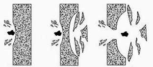
Consider the square barrier shown above. In the regions x < 0 and x > L the wavefunction has the oscillatory behavior we’ve seen before, and can be modeled by linear combinations of sines and cosines. These regions are referred to as allowed regions because the kinetic energy of the particle (KE = E – U) is a real, positive value.

Now consider the region 0 < x < L. In this region, the wavefunction decreases exponentially, and takes the form \[ \Psi(x) = Ae^{-\alpha X}\] This is referred to as a forbidden region since the kinetic energy is negative, which is forbidden in classical physics. However, the probability of finding the particle in this region is not zero but rather is given by: \[P(x) = A^2e^{-2aX}\] Thus, the particle can penetrate into the forbidden region. If the particle penetrates through the entire forbidden region, it can “appear” in the allowed region x > L. This is referred to as quantum tunneling and illustrates one of the most fundamental distinctions between the classical and quantum worlds.

A typical measure of the extent of an exponential function is the distance over which it drops to 1/e of its original value. This occurs when \(x=\frac{1}{2a}\). This distance, called the penetration depth, \(\delta\), is given by \[\delta = \frac{1}{2\alpha}\]

\[\delta = \frac{\hbar x}{\sqrt{8mc^2 (U-E)}}\]

• U is the depth of the potential and
• E is the energy state of the wavefunction.

The penetration depth defines the approximate distance that a wavefunction extends into a forbidden region of a potential. Using this definition, the tunneling probability (T), the probability that a particle can tunnel through a classically impermeable barrier, is given by \[T \approx e^{-x/\delta}\]

For this example, the probability that the proton can pass through the barrier is \[ \delta = \frac{\hbar c}{\sqrt{8mc^2(U-E)}}\]

\[\delta = \frac{197.3 \text{ MeVfm} }{\sqrt{8(938 \text{ MeV}}}(20 \text{ MeV -10 MeV})\]

\[\delta =0.720 \text{ fm}\]

Thus, there is about a one-in-a-thousand chance that the proton will tunnel through the barrier.

Tunneling In and Out

In a crude approximation of a collision between a proton and a heavy nucleus, imagine an 10 MeV proton incident on a symmetric potential well of barrier height 20 MeV, barrier width 5 fm, well depth -50 MeV, and well width 15 fm. Estimate the probability that the proton tunnels into the well. If the proton successfully tunnels into the well, estimate the lifetime of the resulting state.

In this approximation of nuclear fusion, an incoming proton can tunnel into a pre-existing nuclear well. Once in the well, the proton will remain for a certain amount of time until it tunnels back out of the well. Although the potential outside of the well is due to electric repulsion, which has the 1/r dependence shown below,

we will approximate it by a rectangular barrier:

The tunneling probability into the well was calculated above and found to be \[T \approx 0.97x10^{-3}\] All that remains is to determine how long this proton will remain in the well until tunneling back out. First, notice that the probability of tunneling out of the well is exactly equal to the probability of tunneling in, since all of the parameters of the barrier are exactly the same.   Remember, T is now the probability of escape per collision with a well wall, so the inverse of T must be the number of collisions needed, on average, to escape. If we can determine the number of seconds between collisions, the product of this number and the inverse of T should be the lifetime () of the state: The time per collision is just the time needed for the proton to traverse the well. This is simply the width of the well (L) divided by the speed of the proton:

\[ \tau = \bigg( \frac{L}{v}\bigg)\bigg(\frac{1}{T}\bigg)\] The speed of the proton can be determined by relativity,

\[ KE = (\gamma -1)mc^2\]

\[ 60 \text{ MeV} =(\gamma -1)(938.3 \text{ MeV}\]

\[\gamma = 1.064\]

\[v = 0.34c \]

\[v = 1.0 x 10^8 \text{ m/s}\] Therefore the lifetime of the state is: \[ \tau = \bigg( \frac{15 x 10^{-15} \text{ m}}{1.0 x 10^8 \text{ m/s}}\bigg)\bigg( \frac{1}{0.97 x 10^{-3}} \]

\[ \tau = 1.5 x 10^{-19} \text{ s}\]

• Technology Eddy Current Sheet Resistance Calculator Depth of Penetration Calculator FAQ
• Measurements Sheet Resistance Thickness Resistivity Anisotropy Emissivity Weight Permittivity Permeability Residual Moisture
• Products Sheet Resistance Portable Devices Handheld Contact Tester Laboratory Devices Single Point Tester 200 mm Mapping Devices Imaging Device 300 mm Automated Handling Tool 150/200 mm Sensors Inline Monitoring System Inline Wire Testing System Inline Sensorline System Near-process Sensor Integration Accessories Reference Sample Sets Metal Thickness Portable Devices Handheld Contact Tester Laboratory Devices Single Point Tester 200 mm Mapping Devices Imaging Device 300 mm Sensors Inline Monitoring System Resistivity Testing Portable Devices Handheld Contact Tester Laboratory Devices Single Point Tester 200 mm Mapping Devices Imaging Device 300mm Sensors Inline Monitoring System Inline Wire Testing System Accessories Reference Sample Sets Carbon Fiber Laboratory Devices 2D Single Point Fiber Areal Weight Mapping Devices 2D Structural Imaging Sensors 1D Inline Roving, Yarn and Tow 2D Inline Fiber Orientation 2D Inline Gap Detection 2D Fiber Areal Weight Monitoring 3D Fiber Orientation – Robot Integration Software Evaluation Software Multi Parameter Laboratory Devices Single Point Tester 200mm Mapping Devices Imaging Device 300mm Sensors EddyCus® TF inline HF Measurement studies
• About us Company News Press

Penetration Depth Calculator

This tool calculates the Standard Penetration Depth – the depth at which the eddy current density has decreased to 1/e of the surface density – according to the following equation for an eddy current sensor at an operating frequency f:

where f = frequency, µ = permeability, σ = electrical conductivity, µ r = relative permeability,  ω =  angular frequency

The calculator converts theoretical values based on the formular above. We do not vouch for its correctness and applicability to specific conditions.

Penetration depth calculator

Resistivity known, conductivity known.

Similar to 4PP, the eddy current method is also able to determine the resistivity if thickness of the specimen is larger than the penetration depth of the induced currents. The key difference is that the penetration depth of the currents is much smaller than with 4PP setups even if one would use very small tip distances. The penetration depth, meaning the analyzing area for resistivity measurement depends on several factors. The depth of the eddy currents penetrating into a material is affected by the frequency of the eddy currents, the electrical conductivity and magnetic permeability of the specimen.

The depth of penetration decreases with increasing frequency and increasing conductivity and magnetic permeability. The depth at which eddy current density has decreased to 1/e, or about 37% of the surface density, is called the standard depth of penetration (d or 1d) and is used as criteria of ideal measurement for the investigation of bulk materials. At three standard depth of penetration (3d), the eddy current density is down to only 5% of the surface density. Further details are shown in our.

The calculator converts theoretical values based on the laws of physics. We do not vouch for its correctness and applicability to specific conditions.

For product requests contact us by using the

• Contact formular,
• Email ( [email protected] ) or
• Phone (+49 351 32 111 520).

For a prompt and informative response, please describe your measurement task (material, sample dimensions, expected measurement range) and provide your phone number.

By sending this form, I permit SURAGUS GmbH to process my data for contacting me. For more details see our Imprint & Privacy Policy

Product Overview

Privacy policy, chinese website, landing page, applications, carbon fiber testing, thin film characterization.

• Sheet resistance
• Conductivity testing
• Optical transparency

MEASUREMENTS

• Sheet Resistance
• Metal Layer Thickness
• Resistivity
• Electrical Anisotropy
• Permeability
• Coating Weight
• Carbon fiber testing products
• Thin film characterization products

     SIGNUP FOR OUR NEWSLETTER

This website uses cookies. Cookies are used for user guidance and web analysis and help to make this website better. More information and the possibility to object here:  Privacy Policy

Contact Us   Contact Us  

• What is EVIDENT?
• App Marketplace
• Connected Devices
• My Organization
• Evident Connect Log in

Depth of Penetration

Eddy current density does not remain constant across the depth of a material. The density is greatest at the surface and decreases exponentially with depth (the "skin effect"). The standard depth of penetration equation (shown to the right) is used to explain the penetration capability of eddy current testing, which decreases with increasing frequency, conductivity, or permeability. For a material that is both thick and uniform, the standard depth of penetration is the depth at which the eddy current density is 37% of the material surface value. To detect very shallow defects in a material, and also to measure the thickness of thin sheets, very high frequencies are used. Similarly, in order to detect subsurface defects, and to test highly conductive, magnetic, or thick materials, lower frequencies must be used.

Where: d= Standard depth of penetration (mm) f= Test frequency (Hz) mr= Relative magnetic permeability (dimensionless) s= Electrical conductivity (% IACS)

• Subscribe to the Evident email

Redirecting

You are being redirected to our local site.

+49 (421) - 6 88 53 -0 [email protected]

• |   DE
• |   KR
• |   JP
• |   CN

• Physical Basics

Microwave Heating

• Microwave Drying
• Frequency Ranges
• Basic Calculations

Penetration Depths

• GMP - Microwaves
• Conti Dryer / Conti Heater
• Flow Heater / Reactor
• Chamber Ovens
• Vacuum Drying / Freeze-Drying
• Process Control
• Applications
• Publications
• Fairs & events
• Product news
• Privacy Policy

The penetration depth is calculated according to equation (2), which shows how it depends on the dielectric properties of the material. The penetration depth is used to denote the depth at which the power density has decreased to 37 % of its initial value at the surface.

Materials with higher loss factor ε r ’’ (imaginary part of the complex permittivity) show faster microwave energy absorption. The power density will decrease exponentially from the surface to the core region.

Figure 1. Penetration depth (denoted with blue x) of the electric wave decreases with increasing frequency. The left side represents air, the right side a material.

f = frequency, measured in Hz ε O absolute dielectric constant (DC) = 8,85x10-12 As/Vm с = 3x10 10 cm/s speed of light Ε = electrical field strength, measured in V/m ε = ε O * ( ε r ’ - j ε r ’’ ), complex dielectric constant tan δ = ε r ’’/ε r ’ δ = dielectric loss angle, measured in degrees λ 0 = wavelength, measured in, λ 0 =c / f

Table 1 shows the penetration depth values of various materials. It should be noted that the penetration depth of the electric field strength is sometimes reported in the literature, with a value which is twice as high.

Table 1. Penetration depths of microwave energy of various materials at 2450MHz

Products with huge dimensions and high loss factor may occasionally overheat within a considerably thick layer on the outer surface. To prevent such a phenomenon the power density should be chosen so that enough time is provided for the essential heat exchange between boundary and core. If the thickness of the material is less than the penetration depth, only a fraction of the supplied energy will be absorbed.

Nevertheless, this only applies if the energy, which is not absorbed, spread away from the material after leaving it. The unabsorbed microwave radiation is, however, reflected from the metal walls of the application chamber and penetrates the material more than once.

Another consideration of the power density needed for microwave heating is that appropriate field strength values must be maintained inside the application chamber. Under atmospheric conditions, these are generally several orders of magnitude smaller than the breakdown strength for dry air (30 kV/cm). In the case of vacuum applications, or whenever the air inside the applicator is very moist, the electric field strength should be limited to an extent that prevents ionisation of the air, in order to avoid enormous damages that could be caused to both product and equipment.

By using microwave energy, heat is generated inside the product volume by directly transforming the electromagnetic energy into molecular kinetic energy.

Püschner Microwave Heating Advantages

• saves energy because only the product is heated
• compact units save space
• limiting factor "heating" on the process line is eliminated
• flexible modular design
• reliable with an intelligent service and maintenance concept
• environmentally friendly
• gentle on the product because of total volume heating
• high control and process speeds
• minimal delay before ready to use
• rapid heating to operating temperature
• uniform heat distribution

Dielectric Heating

• What to Look for When Buying a GPR System
• What is Subsurface Imaging?
• What is Triple Bandwidth?
• Integrating a 3rd Party GPS
• Building a Map
• Ground Penetrating Radar FAQ

What is the Best GPR System for Me?

• GPRover Utility Mapping System
• Quantum Imager Triple Frequency GPR System
• Q5 Series GPR System
• Q10 Utility and Geotechnical Locating System
• Q25 Geophysical Radar System
• 100 Series Geophysical Scanner
• Utility Locating
• Structural Assessment
• Archaeology
• Geophysical
• Environmental
• Law Enforcement
• Grave Location & Cemetery Mapping
• Radar Acquisition Software
• Radar Studio
• GPS Integration
• 3D Imaging & Modeling
• Third Party Software
• Case Studies
• Trade Shows
• GPR Training
• Tech Support
• Product Registration
• Software Updates

What Is the Effective Depth of Ground Penetrating Radar?

How deep does GPR go? This is one of the most common questions asked surrounding ground-penetrating radar systems and technology. If you’re in the early stages of research, you’ve likely seen a range of answers. What’s more, each answer you find is itself a range. Once you start averaging these ranges together, you’ll likely end up with something between two and 100 feet. Continue reading and visit our site and learn more about GPR and its depth capabilities.

That’s an incredibly high variance. If you’re looking for a solution to help you locate and measure underground objects, you need to know which side of that variance your specific use case falls on. Depth penetration numbers with such a wildly high variance just aren’t helpful. What’s more, without understanding the specific variables that impact GPR penetration depth, they’re even misleading.

Thankfully, grasping those variables and applying them to your survey needs and goals isn’t a time-consuming endeavor. In this case, a little information goes a long way. Here’s what you need to know to determine the depth of GPR penetration for your specific applications.

A Quick Look at How GPR Works in the Field

To understand how the forthcoming variables impact GPR, it’s worth taking a moment to look at how the underlying technology works.

Ground-penetrating radar systems are designed to image subsurface materials using electromagnetic radio waves transmitted into the ground from an antenna. Unlike other systems, GPR analyzes and images the objects within the subsurface layers as well as the layers themselves, including any disturbances within. It’s the best way to nondestructively locate and image subsurface materials and locate the objects within them.

Surveying with a GPR system requires pushing the antenna across the survey site and transmitting the electromagnetic signal into the ground. When the signal encounters some kind of change in the soil — whether an object or an anomaly — it’s bounced back through the soil to the antenna. The system measures the details of this feedback to give clues as to the type of object in the subsurface material as well as its depth.

On higher quality systems, this feedback is displayed in real time on a digital display attached to the system. For example, on our GPRover system , radar feedback is shown as an image on the display. The image updates in real-time, showing distortions in the radar signal, such as hyperbolas or arcs. High and narrow arcs often indicate small, round objects. In contrast, broad, flat arcs indicate much larger objects. Finally, jagged or hyperbolic distortions usually indicate soil or material changes.

Using the GPR’s system software , an operator collects these image distortions and creates datasets that paint a vivid picture of the subsurface material. These datasets determine:

• The location of buried objects
• Depth and dimensions of those objects
• Changes to the structure of the subsurface material

In other words, these datasets provide the necessary information to make informed decisions regarding the survey site, whether it’s locating utility lines for a new construction project or surveying an archeological site for clues. Moreover, the data is sharable with colleagues or stakeholders to help make these decisions.

The Variables That Determine GPR Penetration Depth

Primed with the basics of how everything works, we can look at the variables that impact GPR’s penetration depth in real-world scenarios. While determining the exact depth capabilities of GPR in every possible scenario is an impossible feat, looking at four major variables can narrow things down considerably. Those variables are:

• Material properties and soil conditions
• Target size
• Antenna frequency
• Equipment quality and capability

As you can imagine by looking at the factors above, conditions vary from survey to survey and across a single survey site. If you’re locating objects in various materials or soil conditions at a single survey site, penetration depth varies. But this is why it’s so important to understand each variable.

Material Properties and Soil Conditions

By and large, the biggest variable in determining GPR penetration depth is the material and soil conditions of the survey site. It also affects the quality of the data you collect, so it’s easily the most important consideration for any survey.

Electromagnetic radio waves work like other waves in that they can only travel so far. Eventually, the waves are absorbed by objects or materials in their path. This is where you get the high end of GPR’s depth. In perfect conditions, electromagnetic waves can travel upwards of 100 feet before they’re fully absorbed by the ground.

The other half of the equation is the dielectric properties of the ground material. The dielectric of a material essentially determines how conductive it is. The higher the dielectric of a material, the more conductive it is. And the more conductive a material it is, the more it absorbs the electromagnetic waves of GPR.

When talking about the dielectric properties of ground material, the biggest culprit is moisture. The electromagnetic signal from GPR is absorbed much faster by highly saturated materials, resulting in decreased depth penetration. If you’re scanning a site with dense, wet clay, the impact on penetration depth is considerable. Conversely, if you’re scanning dry material, the depth reaches the higher end of GPR’s capabilities.

Tip : Soil conditions also include factors such as weather. Excessive rainfall can create conditions where even optimal surface materials are too saturated for GPR to work effectively. Keep this in mind when planning a survey.

Target Size

In many cases, surveyors have some idea of the object they’re looking for. It could be a septic tank, utility lines or rebar in cement. In other instances, targets are less defined, such as searching for sinkholes, surveying archeological digs or measuring groundwater. In either case, the target’s size is an important variable to keep in mind.

Put simply, larger objects reflect more electromagnetic waves back to the GPR antenna. Smaller objects still reflect waves, but the reflections are less defined. It’s important to balance this with material properties and soil conditions, too, because even large objects won’t reflect much energy if they’re at the higher end of depth penetration.

Antenna Frequency

There are actually two factors to consider when looking at antenna frequency: depth and data quality. Choosing the frequency that balances these two factors is crucial to effective use of GPR. Of course, you also need to balance these with material properties and soil conditions.

As a general rule, lower frequencies “bounce” less and travel much further than higher frequencies. In perfect conditions, the lower the frequency, the greater the depth. But conditions are seldom perfect. Looking at the example table below, you can see how generally the higher the dielectric of the material, the lower the penetration depth.

So, why not use a 100 MHz antenna and call it good? After all, even in the worst conditions, lower frequencies provide greater depth. The reason is data quality. While lower frequencies travel further, they also provide less information about the materials they travel through and bounce off of. In other words, the lower the frequency, the lower the resolution and the higher likelihood that smaller targets will be missed.

Equipment Capabilities and Quality

The quality and capabilities of the equipment you use are often the deciding factors in the success of your survey. For those who need a solution for a variety of materials and soil conditions, a system that operates on a single frequency will produce unfavorable depth penetration in many situations. And in other instances, it won’t produce the necessary data quality and resolution.

One approach is to use a GPR system that operates on multiple frequency ranges, such as our Quantum Imager . Our solution is equipped with antennas that transmit three separate signals covering the entire range of frequencies used in subsurface imaging. This means you get the best of both worlds: greater depth and higher resolution across a variety of materials and conditions.

On the quality side of things, using a system that’s designed and engineered to a higher standard just makes sense. A higher-quality system produces greater penetration depth, higher resolution data and an easier approach to subsurface imaging. Most importantly, it means consistent and reliable results, survey after survey.

Solutions for Every Scenario With US Radar

A little bit of knowledge goes a long way in helping to understand GPR’s depth penetration capabilities. By looking at the variables that affect those capabilities, you can whittle down the range of numbers into something more appropriate for your specific needs.

At US Radar, we’ve worked hard for more than 30 years to perfect high-quality GPR solutions that produce results in the real world. We know that GPR technology requires a careful balance between the theoretical and the everyday needs of our customers. This is why we offer so many products that work in a variety of applications. If you’d like to find how one of our solutions can work for you, get in touch with us today.

US Radar / Blog / What Is the Effective Depth of Ground Penetrating Radar?

Recommended Reading

April 9, 2024

What is Ground Penetrating Radar (GPR)? Definition & How it Works

January 2, 2023

September 26, 2022

How to Detect Environmental Hazards With GPR

Tech Support Team Lead

Matt is an archaeologist who is the Team Lead for US Radar's Tech Support Department. He holds a BA in Anthropology from Stockton University and a MA in Landscape Archaeology from the University of Galway.