fourier transform example problems and solutions

Fourier Transform | Formula | Examples | Applications

Why fourier transform.

If a function f (t) is not a periodic and is defined on an infinite interval, we cannot represent it by Fourier series . It may be possible, however, to consider the function to be periodic with an infinite period. In this section we shall consider this case in a non-rigorous way, but the results may be obtained rigorously if f (t) satisfies the following conditions:

• $\int\limits_{-\infty }^{\infty }{\left| f(t) \right|}dt$ is finite means $\int\limits_{-\infty }^{\infty }{\left| f(t) \right|}dt<\infty $
• In any finite interval, f(t) has at most a finite number of finite discontinuities
• In any finite interval, f(t) has at most a finite number of maxima and minima
• You May Also Read:  Exponential Fourier Series with Solved Example

Fourier Transform Formula

Let us begin with the exponential series for a function f T (t) defined to be f (t) for

$-T/2<t<T/2$

The result is

${{f}_{T}}(t)=\sum\limits_{-\infty }^{\infty }{{{c}_{n}}{{e}^{{}^{j2\pi nt}/{}_{T}}}}\text{      }\cdots \text{     (1)}$

\[{{c}_{n}}=\frac{1}{T}\int\limits_{-T/2}^{T/2}{{{f}_{T}}(x)}{{e}^{{}^{-j2\pi nx}/{}_{T}}}dx\text{      }\cdots \text{     }(2)\]

We have replaced ω o by 2π/T and are using the dummy variable x instead of t in the coefficient expression. Our intention is to let T→∞, in which case f T (t) →f (t).

Since the limiting process requires that ωo=2π/T→∞, for emphasis we replace 2π/T by ∆ω. Therefore substituting (2) into (1), we have

$\begin{align}  & {{f}_{T}}(t)=\sum\limits_{-\infty }^{\infty }{\left[ \frac{\Delta \omega }{2\pi }\int\limits_{-T/2}^{T/2}{{{f}_{T}}(x)}{{e}^{-jxn\Delta \omega }}dx \right]{{e}^{jtn\Delta \omega }}} \\ & \text{=}\sum\limits_{-\infty }^{\infty }{\left[ \frac{1}{2\pi }\int\limits_{-T/2}^{T/2}{{{f}_{T}}(x)}{{e}^{-j(x-t)n\Delta \omega }}dx \right]}\Delta \omega \text{        }\cdots \text{     (3)} \\\end{align}$

If we define the function

\[g(\omega ,t)=\frac{1}{2\pi }\int\limits_{-T/2}^{T/2}{{{f}_{T}}(x)}{{e}^{-j\omega (x-t)}}dx\text{        }\cdots \text{     }(4)\]

Then clearly the limit of (3) is given by

$f(t)=\underset{T\to \infty }{\mathop{\lim }}\,\sum\limits_{n=-\infty }^{\infty }{g(n\Delta \omega ,t)\Delta \omega \text{        }\cdots \text{     (5)}}$

By the fundamental theorem of integral calculus the last result appears to be

$f(t)=\int\limits_{-\infty }^{\infty }{g(\omega ,t)d}\omega \text{         }\cdots \text{      (6)}$

But in the limit, f T → f and T→∞ in (4) so that what appears to be g (ω, t) in (6) is really its limit, which by (4) is

\[\underset{T\to \infty }{\mathop{\lim }}\,g(\omega ,t)=\frac{1}{2\pi }\int\limits_{-\infty }^{\infty }{f(x)}{{e}^{-j\omega (x-t)}}dx\]

Therefore (6) is actually

$f(t)=\frac{1}{2\pi }\int\limits_{-\infty }^{\infty }{\left[ \int\limits_{-\infty }^{\infty }{f(x)}{{e}^{-j\omega (x-t)}}dx \right]d}\omega \text{         }\cdots \text{      (7)}$

As we said, this is non-rigorous development, but the results may be obtained rigorously.

Let us rewrite (7) in the form

$f(t)=\frac{1}{2\pi }\int\limits_{-\infty }^{\infty }{\left[ \int\limits_{-\infty }^{\infty }{f(x)}{{e}^{-j\omega x}}dx \right]{{e}^{j\omega t}}d}\omega \text{         }\cdots \text{      (8)}$

Now, let us define the expression in brackets to be the function

  [stextbox id=”info” caption=”Fourier Transform “]\[F(j\omega )=\int\limits_{-\infty }^{\infty }{f(t){{e}^{-j\omega t}}dt}\text{         }\cdots \text{    }(9)\][/stextbox]

Where we have changed the dummy variable from x to t. then (8) becomes

  [stextbox id=”info” caption=”Inverse Fourier Transform “]\[f(t)=\frac{1}{2\pi }\int\limits_{-\infty }^{\infty }{F(j\omega ){{e}^{j\omega t}}}d\omega \text{       }\cdots \text{    (10)}\][/stextbox]

The function F (jω) is called the Fourier Transform of f (t), and f (t) is called the inverse Fourier Transform of F (jω). These facts are often stated symbolically as

$\begin{matrix}   \begin{align}  & F(j\omega )=\Im [f(t)] \\ & f(t)={{\Im }^{-1}}[F(j\omega )] \\\end{align} & \cdots  & (11)  \\\end{matrix}$

Also, (9) and (10) are collectively called the Fourier Transform Pair, the symbolism for which is

$f(t)\leftrightarrow F(j\omega )\text{          }\cdots \text{     (12)}$

The expression in (7), called the Fourier Integral, is the analogy for a non-periodic f (t) to the Fourier series for a periodic f (t). Equation (10) is, of course, another form of (7). Another description for these analogies is to say that the Fourier Transform is a continuous representation (ω being a continuous variable), whereas the Fourier series is a discrete representation (nω o , for n an integer, being a discrete variable).

Fourier Transform Example

As an example, let us find the transform of

$f(t)={{e}^{-at}}u(t)$

Whereas a>0. By definition we have

$\begin{align}  & \Im [{{e}^{-at}}u(t)]=\int\limits_{-\infty }^{\infty }{{{e}^{-at}}u(t){{e}^{-j\omega t}}dt} \\ & =\int\limits_{0}^{\infty }{{{e}^{-(a+j\omega )t}}dt} \\\end{align}$

$\Im [{{e}^{-at}}u(t)]=\left. \frac{1}{-(a+j\omega )}{{e}^{-(a+j\omega )t}} \right|_{0}^{\infty }$

The upper limit is given by

$\underset{t\to \infty }{\mathop{\lim }}\,{{e}^{-at}}(\cos \omega t-j\sin \omega t)=0$

Since the expression in parentheses is bounded while the exponential goes to zero. Thus we have

$\Im [{{e}^{-at}}u(t)]=\frac{1}{(a+j\omega )}$

\[{{e}^{-at}}u(t)\leftrightarrow \frac{1}{(a+j\omega )}\]

Fourier Transform Applications

The Fourier transform is used in various fields and applications where the analysis of signals or data in the frequency domain is required. Some common scenarios where the Fourier transform is used include:

Signal Processing: Fourier transform is extensively used in signal processing to analyze and manipulate signals. It allows the decomposition of a signal into its frequency components, enabling tasks such as filtering, noise removal, compression, and modulation/demodulation.

Communication Systems: In communication systems, the Fourier transform is used for signal modulation and demodulation. It helps convert signals between the time and frequency domains, enabling efficient transmission and reception of information.

Image Processing: Fourier transform finds applications in image processing for tasks like image enhancement, compression, and restoration. It allows the analysis and manipulation of image frequency components for various image processing operations.

Audio Processing: Fourier transform is used in audio processing for tasks like audio compression (e.g., MP3), equalization, noise removal, and audio effects. It enables the representation of audio signals in the frequency domain, allowing precise control over different frequency components.

Physics and Engineering: Fourier transform is extensively used in physics and engineering fields to analyze physical phenomena and systems. It helps in understanding wave behavior, studying vibrations and resonance , analyzing system responses, and solving differential equations in frequency domain.

Data Analysis: Fourier transform is applied in data analysis tasks such as spectrum analysis, feature extraction, and pattern recognition. It helps identify dominant frequency components in data, reveal underlying patterns, and extract meaningful information from complex datasets.

Quantum Mechanics: Fourier transform plays a crucial role in quantum mechanics, particularly in understanding the wave-particle duality and the mathematical representation of quantum states.

These are just a few examples of the broad range of applications where the Fourier transform is used. Its ability to analyze signals in the frequency domain makes it a valuable tool in various scientific, engineering, and mathematical disciplines.

• You May Also Read:  Trigonometric Fourier Series Solved Examples

Leave a Comment Cancel reply

You must be logged in to post a comment.

CT Fourier transform practice problems list - Rhea

• View source
• Recent Changes

CT Fourier transform practice problems list

Practice Problems

on continuous-time Fourier transform

(Function of $ \omega $ in radian per time unit)

Collectively solved problems on continuous-time Fourier transform

• Compute the Fourier transform of e^-t u(t)
• Compute the Fourier transform of cos(2 pi t).
• Compute the Fourier transform of cos(2 pi t + pi/12).
• Compute the Fourier transform of a rectangular pulse-train
• Compute the Fourier transform of a triangular pulse-train
• Derive a relationship between the FT of x(3t+7) and that of x(t)

Problems invented and by students: can you find the mistakes?

• Computation of CT Fourier transform
• Computation of Inverse CT Fourier transform

Back to Practice Problems on "Signals and Systems"

• Signals and systems
• Problem solving
• Fourier transform
• Inverse Fourier transform

Alumni Liaison

Browse Course Material

Course info.

• Prof. Alan V. Oppenheim

Departments

• Supplemental Resources

As Taught In

• Digital Systems
• Signal Processing
• Computational Modeling and Simulation

Learning Resource Types

Signals and systems, assignments.

You are leaving MIT OpenCourseWare

• school Campus Bookshelves
• menu_book Bookshelves
• perm_media Learning Objects
• login Login
• how_to_reg Request Instructor Account
• hub Instructor Commons

Margin Size

• Download Page (PDF)
• Download Full Book (PDF)
• Periodic Table
• Physics Constants
• Scientific Calculator
• Reference & Cite
• Tools expand_more
• Readability

selected template will load here

This action is not available.

5.E: Fourier Transform (Exercises)

• Last updated
• Save as PDF
• Page ID 2155

• Erich Miersemann
• University of Leipzig

\( \newcommand{\vecs}[1]{\overset { \scriptstyle \rightharpoonup} {\mathbf{#1}} } \)

\( \newcommand{\vecd}[1]{\overset{-\!-\!\rightharpoonup}{\vphantom{a}\smash {#1}}} \)

\( \newcommand{\id}{\mathrm{id}}\) \( \newcommand{\Span}{\mathrm{span}}\)

( \newcommand{\kernel}{\mathrm{null}\,}\) \( \newcommand{\range}{\mathrm{range}\,}\)

\( \newcommand{\RealPart}{\mathrm{Re}}\) \( \newcommand{\ImaginaryPart}{\mathrm{Im}}\)

\( \newcommand{\Argument}{\mathrm{Arg}}\) \( \newcommand{\norm}[1]{\| #1 \|}\)

\( \newcommand{\inner}[2]{\langle #1, #2 \rangle}\)

\( \newcommand{\Span}{\mathrm{span}}\)

\( \newcommand{\id}{\mathrm{id}}\)

\( \newcommand{\kernel}{\mathrm{null}\,}\)

\( \newcommand{\range}{\mathrm{range}\,}\)

\( \newcommand{\RealPart}{\mathrm{Re}}\)

\( \newcommand{\ImaginaryPart}{\mathrm{Im}}\)

\( \newcommand{\Argument}{\mathrm{Arg}}\)

\( \newcommand{\norm}[1]{\| #1 \|}\)

\( \newcommand{\Span}{\mathrm{span}}\) \( \newcommand{\AA}{\unicode[.8,0]{x212B}}\)

\( \newcommand{\vectorA}[1]{\vec{#1}}      % arrow\)

\( \newcommand{\vectorAt}[1]{\vec{\text{#1}}}      % arrow\)

\( \newcommand{\vectorB}[1]{\overset { \scriptstyle \rightharpoonup} {\mathbf{#1}} } \)

\( \newcommand{\vectorC}[1]{\textbf{#1}} \)

\( \newcommand{\vectorD}[1]{\overrightarrow{#1}} \)

\( \newcommand{\vectorDt}[1]{\overrightarrow{\text{#1}}} \)

\( \newcommand{\vectE}[1]{\overset{-\!-\!\rightharpoonup}{\vphantom{a}\smash{\mathbf {#1}}}} \)

These are homework exercises to accompany Miersemann's " Partial Differential Equations " Textmap. This is a textbook targeted for a one semester first course on differential equations, aimed at engineering students. Partial differential equations are differential equations that contains unknown multivariable functions and their partial derivatives. Prerequisite for the course is the basic calculus sequence.

\[ \int_{{\mathbb{R}}^n}{\rm e}^{-|y|^2/2}\ dy=(2\pi)^{n/2}. \]

Show that \(u\in \mathcal{S}(\mathbb{R}n^)\) implies \(\hat{u},\ \widetilde{u}\in\mathcal{S}(\mathbb{R}^n)\).

Give examples for functions \(p(x,\xi)\) which satisfy \(p(x,\xi)\in S^m\).

Find a formal solution of Cauchy's initial value problem for the wave equation by using Fourier's transform.

Contributors:

• Prof. Dr. Erich Miersemann ( Universität Leipzig )

Integrated by Justin Marshall.

• Machine Learning Decision Tree – Solved Problem (ID3 algorithm)
• Poisson Distribution | Probability and Stochastic Process
• Conditional Probability | Joint Probability
• Solved assignment problems in communicaion |online Request
• while Loop in C++

EngineersTutor

Fourier transform solved problems | signals & systems.

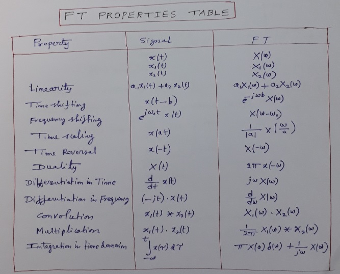
• ← Fourier transform properties | Part 2 | Signals & Systems
• DTFT | Discrete Time Fourier Transform →

Gopal Krishna

Hey Engineers, welcome to the award-winning blog,Engineers Tutor. I'm Gopal Krishna. a professional engineer & blogger from Andhra Pradesh, India. Notes and Video Materials for Engineering in Electronics, Communications and Computer Science subjects are added. "A blog to support Electronics, Electrical communication and computer students".

You May Also Like

Invertible – inverse systems | stable – unstable systems | signals and systems, fourier transform properties | linearity | time scaling, properties of systems | causal | non-causal |signals & systems, leave a reply cancel reply.

Your email address will not be published. Required fields are marked *