case study on montreal protocol

September 23, 2022

How the Montreal Protocol Helped Save Earth from a Climate Time Bomb

The landmark Montreal Protocol treaty, agreed to 35 years ago this month, has reduced the use of chemicals that not only thinned the ozone layer but also warmed the planet

By Jean Chemnick & E&E News

The Antarctic ozone hole on October 2, 2015 as captured by the Aura satellite.

World History Archive/Alamy Stock Photo

The Montreal Protocol didn’t just preserve the ozone layer, it helped save Earth from a climate change time bomb.

The landmark ozone treaty was agreed 35 years ago this month, at a time when both climate and ozone science was far less developed than it is today. Yet every nation signed on, accepting binding commitments to reduce the production, consumption and emissions of chemicals responsible for thinning the ozone layer that guards the planet from the sun’s most damaging radiation. The same set of chemicals happened also to be immensely powerful greenhouse gases, and cutting them bought the world valuable time to deal with the climate crisis.

“If we let the [chlorofluorocarbons (CFCs)] keep growing, we would have had the impacts of climate change that we’re feeling now ... a decade ago,” said David Doniger, a lawyer with the Natural Resources Defense Council who has worked on the issue since the 1980s. “And things would be that much worse now.”

On supporting science journalism

If you're enjoying this article, consider supporting our award-winning journalism by subscribing . By purchasing a subscription you are helping to ensure the future of impactful stories about the discoveries and ideas shaping our world today.

The protocol’s status as a climate treaty was enhanced by the 2016 Kigali Amendment—named for the Rwandan capital where the deal was drafted—which targeted a class of coolants that weren’t ozone-depleting but were climate-forcing. Scientists say the global hydrofluorocarbon (HFCs) phasedown, which the U.S. is now poised to join after a key Senate vote Wednesday, has the potential to avoid half a degree Celsius of warming by 2100.

Scientists, lawyers and others who have worked on the issue for decades say that long before international negotiators struck the deal on HFCs, the ozone treaty had prevented a particularly harmful set of climate superpollutants from being baked into the air conditioning and refrigerators that developing countries were at last acquiring.

David Fahey, director of NOAA’s Chemical Sciences Laboratory and co-chair of the Montreal Protocol’s scientific assessment panel, was among the scientists who in 1987 flew a NASA research aircraft into the ozone hole that had appeared over Antarctica. There were at the time several competing theories for why the hole was appearing, he said.

But the NASA journey, he said, “created a smoking gun plot, as we call it, that was really the pivotal evidence that chlorine was destroying ozone on the scale of what would cause the Antarctic ozone hole.”

The world responded quickly.

“The same month we were in southern Chile flying into Antarctica, in Montreal the Montreal Protocol was being signed,” he said. “And it was basically signed without knowing for sure what was causing the Antarctic ozone hole.”

The new agreement was not only a leap of faith as far as the science was concerned, but it had attributes that have never been replicated in any subsequent climate treaty despite far higher levels of scientific certainty.

The treaty is universal with 197 member countries. It is legally binding with penalties for countries that flout its provisions. And it is fully funded, meaning that poorer countries that might not have been able to meet its targets to phase down chemicals received assistance from richer ones.

“There’s no other forum that has those three dimensions,” Fahey said, noting the 2015 Paris Agreement on climate change relies on voluntary commitments with no penalties for breaking them.

“Probably the underlying problem with the climate change situation is we don’t have such a forum,” he said.

DuPont scientist’s key role

Fahey said there was some understanding among scientists from the start that CFCs played a role in driving climate change as well as depleting the ozone layer. But that role was clarified by a scientific study that he and four other scientists published in 2007, which looked at the “worlds avoided” by stemming the growth of the chemicals.

The report showed that without the Montreal Protocol, CFC use would have ballooned. Under a conservative scenario by 2010, the chemicals would have had a greenhouse gas content nearly equal to half the carbon dioxide emissions from all other sources. The effect on the climate would have been catastrophic.

“I think the estimates are something on the order of an extra 2 degrees by the middle of the century,” said Susan Solomon, a professor of environmental studies at the Massachusetts Institute of Technology.

She noted that had the world continued on its trajectory of increasing CFC use through 2050, the consequences for the ozone layer would have threatened the health and survival of every living thing on the planet, including humans. That might have forced action, she said.

“The great news is that we avoided all of that, and we not only saved the ozone layer, we actually had a tremendous win for the climate as well,” she said.

While CFCs packed the biggest punch on climate change, the hydrochlorofluorocarbons (HCFCs) that temporarily replaced them still had significant consequences for the climate. After the 2007 paper was published, parties to the Montreal Protocol quickly moved to shorten the treaty’s timeline for phasing down HCFCs, an adjustment that Fahey said was the first decision made under the Montreal Protocol to reduce global warming.

HCFCs were replaced by HFCs. And HFCs, which have no effect on the ozone, were intended to be the Montreal Protocol’s final destination. But they’re climate superpollutants that can be thousands of times as potent as carbon dioxide.

Industry was initially resistant to the idea that HFC use would have a significant impact on climate change. But Fahey credits an industry scientist, Mack McFarland of DuPont, with changing the discussion.

“The thing that Mack understood was the growth in the developing world,” he said. “That the developing world was catching up with the developed world.”

McFarland started talking to delegates at the annual Montreal Protocol meetings about the role HFCs could eventually play in driving climate change, Fahey said.

“This became one of his main messages to not only the delegates, but to the scientists and to the technologists,” he said. “And it wasn’t extremely well-received or immediately received. And even the scientists—I being one of them—didn’t really get it, so to speak.”

But in 2009, McFarland, Fahey and the other scientists who had collaborated on the 2007 paper on the climate implications of the protocol published a paper on the effects of running the world’s air condition and refrigeration units on HFCs. And its conclusions sparked the negotiations that finally led to the Kigali Amendment’s creation eight years later.

Solomon said she was shocked when the Senate voted this week by a 69-27 margin to join the Kigali treaty. The accord took effect Jan. 1, 2019, after reaching a ratification threshold. The U.S. is the 138th country to sign on.

But Solomon said that in the 1970s and ‘80s, the U.S. led the charge on global ozone protection.

“I think the primary credit needs to go to the American people,” she said.

Help for poor countries

When ozone science was in its infancy, not long after scientists Sherwood Rowland and Mario Molina demonstrated in 1974 that CFC damaged the ozone, but before the extent of the damage was known, U.S. consumers stopped buying aerosol deodorant and hair spray.

The consequences were transformational. U.S. personal care products made up 75 percent of global CFC use in 1974. Plunging demand forced industry to seek alternatives and made the Montreal Protocol possible.

And countries that now project leadership on climate change and other issues clung to their aerosol products.

“The Europeans were actually on the other side of the negotiating table,” Solomon said. “It was us saying, ‘We should get rid of these compounds, we have substitutes, let’s move on. Let’s save the planet.’ And it was Europe saying, ‘Well, you know, we don’t really see that need the way you do.’”

Solomon also credited former President Barack Obama and former Secretary of State John Kerry with creating the geopolitical momentum that carried Kigali across the finish line.

Nor are the direct climate benefits of the protocol’s cuts in CFCs, HCFCs and now HFCs the full story.

Solomon pointed out that the protocol’s multilateral fund helped poor countries gain access to refrigeration, reducing emissions from food waste and spoilage.

NRDC’s Doniger referenced a study published  in  Nature  last year that found that without the ozone preservation benefits of the Montreal Protocol, much less CO 2 would have been absorbed over the past 35 years as the world’s biosphere disintegrated.

“The damage done to trees and other vegetation would have meant that they would have soaked up a lot less CO 2 from the atmosphere,” he said.

The  Nature  study argues that the protocol helped avoid 2.5 degrees Celsius of warming. For context, scientists have warned that the world—and especially vulnerable countries—will face catastrophic damages if warming exceeds 1.5 C.

Reprinted from  E&E News  with permission from POLITICO, LLC. Copyright 2022. E&E News provides essential news for energy and environment professionals.

Scientific Assessment of Ozone Depletion: 2022

Executive summary, recommended citation, executive summary citation:.

World Meteorological Organization (WMO), Executive Summary. Scientific Assessment of Ozone Depletion: 2022 , GAW Report No. 278, 56 pp., WMO, Geneva, Switzerland, 2022.

Science has been one of the foundations of the Montreal Protocol's success. This document highlights advances and updates in the scientific understanding of ozone depletion since the 2018 Scientific Assessment of Ozone Depletion and provides policy-relevant scientific information on current challenges and future policy choices.

Major Achievements of the Montreal Protocol

• Actions taken under the Montreal Protocol continued to decrease atmospheric abundances of controlled ozone-depleting substances (ODSs) and advance the recovery of the stratospheric ozone layer. The atmospheric abundances of both total tropospheric chlorine and total tropospheric bromine from long-lived ODSs have continued to decline since the 2018 Assessment. New studies support previous Assessments in that the decline in ODS emissions due to compliance with the Montreal Protocol avoids global warming of approximately 0.5-1 °C by mid-century compared to an extreme scenario with an uncontrolled increase in ODSs of 3-3.5% per year.
• Actions taken under the Montreal Protocol continue to contribute to ozone recovery. Recovery of ozone in the upper stratosphere is progressing. Total column ozone (TCO) in the Antarctic continues to recover, notwithstanding substantial interannual variability in the size, strength, and longevity of the ozone hole. Outside of the Antarctic region (from 90°N to 60°S), the limited evidence of TCO recovery since 1996 has low confidence. TCO is expected to return to 1980 values around 2066 in the Antarctic, around 2045 in the Arctic, and around 2040 for the near-global average (60°N-60°S). The assessment of the depletion of TCO in regions around the globe from 1980-1996 remains essentially unchanged since the 2018 Assessment.
• Compliance with the 2016 Kigali Amendment to the Montreal Protocol, which requires phase down of production and consumption of some hydrofluorocarbons (HFCs), is estimated to avoid 0.3-0.5°C of warming by 2100. This estimate does not include contributions from HFC-23 emissions.

Current Scientific and Policy Challenges

• The recent identification of unexpected CFC-11 emissions led to scientific investigations and policy responses. Observations and analyses revealed the source region for at least half of these emissions and substantial emissions reductions followed. Regional data suggest some CFC-12 emissions may have been associated with the unreported CFC-11 production. Uncertainties in emissions from banks and gaps in the observing network are too large to determine whether all unexpected emissions have ceased.
• Unexplained emissions have been identified for other ODSs (CFCs-13, 112a, 113a, 114a, 115, and CCl 4 ), as well as HFC-23. Some of these unexplained emissions are likely occurring as leaks of feedstocks or by-products, and the remainder is not understood.
• Outside of the polar regions, observations and models are in agreement that ozone in the upper stratosphere continues to recover. In contrast, ozone in the lower stratosphere has not shown signs of recovery. Models simulate a small recovery in mid-latitude lower-stratospheric ozone in both hemispheres that is not seen in observations. Reconciling this discrepancy is key to ensuring a full understanding of ozone recovery.
• The existing network of atmospheric monitoring stations provides measurements of global surface concentrations of long-lived ODSs and HFCs resulting from anthropogenic emissions. However, gaps in regional atmospheric monitoring limit the scientific community's ability to identify and quantify emissions of controlled substances from many source regions.
• Several space-borne instruments providing vertically resolved, global, measurements of ozone-related atmospheric constituents (e.g., reactive chlorine, water vapor, and long-lived transport tracers) are due to be retired within a few years. Without replacements of these instruments, the ability to monitor and explain changes in the stratospheric ozone layer in the future will be impeded.
• The impact on the ozone layer of stratospheric aerosol injection (SAI), which has been proposed as a possible option to offset global warming, has been assessed following the terms of reference for the 2022 SAP Assessment Report. Important potential consequences, such as deepening of the Antarctic ozone hole and delay in ozone recovery, were identified. Many knowledge gaps and uncertainties prevent a more robust evaluation at this time.
• Heightened concerns about influences on 21st century ozone include impacts of: further increases in nitrous oxide (N 2 O), methane (CH 4 ), and CO 2 concentrations; rapidly expanding ODS and HFC feedstock use and emissions; climate change on TCO in the tropics; extraordinary wildfires and volcanic eruptions; increased frequency of civilian rocket launches and the emissions of a proposed new fleet of supersonic commercial aircraft.

Future Policy Considerations

• If ODS feedstock emissions as currently estimated were to be eliminated in future years, the return of mid-latitude Equivalent Effective Stratospheric Chlorine (EESC) to 1980 abundances could be advanced by almost 4 years, largely due to reductions in CCl 4 , and thereby reduce total climate forcing from ODSs.
• Eliminating future emissions of methyl bromide (CH 3 Br) from quarantine and pre-shipment applications currently allowed by the Montreal Protocol would accelerate the return of mid-latitude EESC to 1980 abundances by two years (as noted in previous Assessments).
• Emissions of anthropogenic very short-lived chlorine substances, dominated by dichloromethane (CH 2 Cl 2 ), continue to grow and contribute to ozone depletion. If CH 2 Cl 2 emissions continue at their current level, they will continue to deplete approximately 1 DU of annually averaged global TCO. Elimination of these emissions would rapidly reverse this depletion.
• A 3% reduction in anthropogenic N 2 O emission, averaged over 2023-2070, would lead to an increase in annually averaged global TCO of about 0.5 DU over the same period, and a decrease of about 0.04 Wm -2 in radiative forcing, averaged over 2023-2100.
• Global emissions of long-lived HFC-23, which are largely a byproduct of HCFC-22 production, are as much as eight times larger than expected and are likely to grow unless abatement increases during HCFC-22 production or feedstock use of HCFC-22 decreases.

This document contains information upon which the Parties to the Montreal Protocol on Substances that Deplete the Ozone Layer ("The Parties") will base their future decisions regarding protection of the stratospheric ozone layer and climate from the production and consumption of ozone-depleting substances (ODSs) and their replacements.

The Charge to the Assessment Panels

Specifically, Article 6 of the Montreal Protocol on Substances that Deplete the Ozone Layer states:

Beginning in 1990, and at least every four years thereafter, the Parties shall assess the control measures provided for in Article 2 and Articles 2A to 2I on the basis of available scientific, environmental, technical and economic information.

To provide the mechanisms whereby these assessments are conducted, the Montreal Protocol further states:

". . . the Parties shall convene appropriate panels of experts" and "the panels will report their conclusions . . . to the Parties."

To meet this request, the Scientific Assessment Panel (SAP), the Environmental Effects Assessment Panel, and the Technology and Economic Assessment Panel each prepare, every 4 years, major assessments that update the state of understanding in their purviews. These assessments are made available to the Parties in advance of their annual meetings at which they consider amendments and adjustments to the provisions of the Montreal Protocol.

Sequence of Scientific Assessments

The 2022 Assessment is the latest in a series of assessments prepared by the world's leading scientific experts and under the auspices of the Montreal Protocol in coordination with the World Meteorological Organization (WMO) and/or the United Nations Environment Programme (UN Environment). The 2022 Assessment is the tenth in the series of major assessments that have been prepared by the Scientific Assessment Panel as direct input to the Montreal Protocol process. The chronology of the ten scientific assessments of ozone depletion, along with other relevant reports and international policy decisions, are summarized in Table ES-1 .

2022 Assessment Terms of Reference

The terms of reference of the 2022 Assessment for the SAP were decided at the 31st Meeting of the Parties to the Montreal Protocol in Rome, Lazio, Italy (4-8 November 2019) in their Decision XXXI/2 1 (items 1-3 and 5):

1. To request the Scientific Assessment Panel, the Environmental Effects Assessment Panel and the Technology and Economic Assessment Panel to prepare quadrennial assessment reports and submit them to the Secretariat by 31 December 2022 for consideration by the Open-ended Working Group and the Meeting of the Parties in 2023, and to present a synthesis report by 30 April 2023, noting that the panels should continue to exchange information, during the process of developing their respective reports in order to avoid duplication and provide comprehensive information to the parties to the Montreal Protocol;

2. To request the assessment panels to bring to the notice of the parties any significant developments which, in their opinion, deserve such notice, in accordance with decision IV/13;

3. To encourage the assessment panels to closely involve relevant scientists from Article 5 parties with a view to promoting gender and regional balance, to the best of their ability, in producing the reports;

5. That the 2022 report of the Scientific Assessment Panel should include: An assessment of the state of the ozone layer and its future evolution; An evaluation of global and polar stratospheric ozone, including the Antarctic ozone hole and Arctic winter/ spring ozone depletion and the predicted changes in those phenomena; An evaluation of trends in the top-down derived emissions, abundances and fate in the atmosphere of trace gases of relevance to the Montreal Protocol on Substances that Deplete the Ozone Layer, in particular controlled substances and other substances of importance to the ozone layer, which should include a comparison of bottom-up and top-down estimations of such emissions with a view to addressing unidentified emission sources and discrepancies between reported emissions and observed atmospheric concentrations; An evaluation of consistency with reported production and consumption of those substances and the likely implications for the state of the ozone layer, including its interaction with the climate system; An assessment of the interaction between changes in stratospheric ozone and the climate system, including possible future policy scenarios relating to ozone depletion and climate impacts; Early identification and quantification, where possible, of any other issues of importance to the ozone layer and the climate system consistent with the objectives of the Vienna Convention for the Protection of the Ozone Layer and the Montreal Protocol; An assessment of information and research related to solar radiation management and its potential effect on the stratospheric ozone layer; Relevant information on any newly detected substances that are relevant for the Montreal Protocol.

The Assessment Process

The process of writing the current Assessment started early in 2020. The co-chairs of the Scientific Assessment Panel (SAP) of the Montreal Protocol (David W. Fahey, Paul A. Newman, John A. Pyle, and Bonfils Safari) considered suggestions from the Parties regarding experts from their countries who could participate in the process. A Scientific Steering Committee (SSC), comprising the co-chairs and an ad-hoc international scientific advisory group, was formed to suggest authors and reviewers from the world scientific community and to help craft the Assessment outline. As in previous Assessments, the participants represented experts from the developed and developing world who bring a special perspective to the process and whose involvement in the Assessment contributes to capacity building. The Authors, Contributors, and Reviewers section at the end of this document provides a listing of the approximately 230 scientists from 30 countries who contributed to the preparation and review of the Assessment.

An initial letter was sent to a large number of scientists and policymakers in November 2020 soliciting comments and inputs on a draft outline along with suggestions for authors for the 2022 Assessment. This was followed by revisions to the outline and recruitment of lead authors and co-authors. Revised chapter outlines were developed between February and April 2021 through a series of online meetings of the SSC and lead authors. The chapter writing process produced four drafts between August 2021 and September 2022 aided by a virtual meeting of the author team and SSC in March 2022 and an in-person meeting in July 2022 at WMO Headquarters in Geneva, Switzerland. The first drafts of the chapters were formally peer-reviewed by over 100 expert reviewers. The chapters were revised by the author teams based on the extensive review comments (numbering over 3500). Review editors for each chapter provided oversight of the revision process to ensure that all comments were addressed appropriately.

At a meeting in Geneva, Switzerland, held on 25-29 July 2022, the Executive Summary contained herein was prepared and completed by the 74 attendees of the meeting. These attendees included the steering committee, chapter lead authors, review editors, some chapter co-authors (selected by the chapter leads), reviewers (selected by the review editors), and some leading experts invited by the steering committee. The Executive Summary, initially drafted by the Assessment SSC, was reviewed, revised, and approved line-by-line. The Highlights section was drafted during the meeting to provide a concise summary of the Executive Summary.

The success of the 2022 Assessment depended on the combined efforts and commitment of a large international team of scientific researchers who volunteered their time as lead authors, contributors, reviewers, and review editors and on the skills and dedication of the assessment coordinator and the editorial and production staff, who are listed at the end of this report.

Table ES-1. Chronology of scientific reports and policy decisions related to ozone depletion.

Introduction

The 1985 Vienna Convention for the Protection of the Ozone Layer is an international agreement in which United Nations States recognized the fundamental importance of preventing damage to the stratospheric ozone layer. The 1987 Montreal Protocol on Substances that Deplete the Ozone Layer and its succeeding amendments, adjustments, and decisions were subsequently negotiated to control the consumption and production of anthropogenic ozone-depleting substances (ODSs) and some hydrofluorocarbons (HFCs). The Montreal Protocol Parties base their decisions on scientific, environmental, technical, and economic information that is provided by their technical panels. The Protocol requests quadrennial reports from its Scientific Assessment Panel that update the science of the ozone layer. This Executive Summary (ES) highlights the key findings of the Scientific Assessment of Ozone Depletion: 2022 , as put together by an international team of scientists. The key findings of each of the six chapters of the Scientific Assessment have been condensed and formulated to make the ES suitable for a broad audience.

Ozone depletion is caused by human-related emissions of ODSs and the subsequent release of reactive halogen gases, especially chlorine and bromine, in the stratosphere. ODSs include chlorofluorocarbons (CFCs), bromine- containing halons and methyl bromide, hydrochlorofluorocarbons (HCFCs), carbon tetrachloride (CCl 4 ), and methyl chloroform. The substances controlled under the Montreal Protocol are listed in the various annexes to the agreement (CFCs and halons under Annex A and B, HCFCs under Annex C, and methyl bromide under Annex E) 2 . These ODSs are long-lived (e.g., CFC-12 has a lifetime greater than 100 years) and are also powerful greenhouse gases (GHGs). As a consequence of Montreal Protocol controls, the stratospheric concentrations of anthropogenic chlorine and bromine are declining.

In addition to the longer-lived ODSs, there is a broad class of chlorine- and bromine-containing substances known as very short-lived substances (VSLSs) that are not controlled under the Montreal Protocol and have lifetimes short- er than about 6 months. For example, bromoform (CHBr 3 ) has a lifetime of 24 days, while chloroform (CHCl 3 ) has a lifetime of 149 days. These substances are generally destroyed in the lower atmosphere in chemical reactions. In general, only small fractions of VSLS emissions reach the stratosphere where they contribute to chlorine and bro- mine levels and lead to increased ozone depletion.

The Montreal Protocol's control of ODSs stimulated the development of replacement substances, firstly HCFCs and then HFCs, in a number of industrial sectors. While HFCs have only a minor effect on stratospheric ozone, some HFCs are powerful GHGs. Previous Assessments have shown that HFCs have been increasing rapidly in the atmosphere over the last decade and were projected to increase further as global development continued in the coming decades. The adoption of the 2016 Kigali Amendment to the Montreal Protocol (see Annex F) will phase down the production and consumption of some HFCs and avoid much of the projected global increase and associated climate change.

Observations of atmospheric ozone are made by instruments on the ground and on board balloons, aircraft, and satellites. This network of observations documented the decline of ozone around the globe, with extreme depletions occurring over Antarctica in each spring and occasional large depletions in the Arctic, and they allowed us to report some indications of recovery in stratospheric ozone in the 2014 and 2018 Assessments. The chemical and dynamical processes controlling stratospheric ozone are well understood, with ozone depletion being fundamentally driven by the atmospheric abundances of chlorine and bromine.

Strong declines in the emissions of ODSs starting in the late 1980s lead to a decline in the abundances of chlorine and bromine starting around the turn of the century. As a result, the first indications of ozone recovery are emerging. In addition to ODSs, model simulations demonstrate that stratospheric ozone concentrations are also affected by the chemical and climate effects of greenhouse gases. In particular, increasing concentrations of the GHGs carbon dioxide (CO 2 ) and methane (CH 4 ) during this century will cause global ozone levels to increase beyond the natural level of ozone observed in the 1960s, primarily because of the cooling of the upper stratosphere and a change of the stratospheric circulation. On the other hand, the chemical effect of increasing concentrations of nitrous oxide (N 2 O), another GHG, will be to deplete stratospheric ozone.

This 2022 Assessment is the tenth in a series that is provided to the Montreal Protocol by its Scientific Assessment Panel. Completely new to this Assessment is Chapter 6, on the potential effects on ozone of the intentional addition of aerosols to the stratosphere, known as stratospheric aerosol injection (SAI). SAI has been proposed as a potential method to reduce climate warming by increasing sunlight reflection; an unintended consequence of SAI is that it could also affect stratospheric temperatures, circulation and ozone production and destruction rates and transport. This new chapter assesses our understanding of these effects based on the SAI strategy and under different climate warming scenarios, as well as identifying sources of uncertainty in these impacts.

In the other six chapters of this Assessment, many of our previous Assessment findings are strengthened and new results are presented. A clear message of the 2022 Assessment is that the Montreal Protocol continues to be effective at reducing the atmospheric abundance of ODSs.

[1] Abundances and trends in ozone-depleting substances (ODSs)

Our confidence in the achievements of the Montreal Protocol continues to be based on sustained networks of measurements of long-lived source gas abundances covering several decades. These measurements allow the determination of global abundances, their interhemispheric differences and their trends. The data allow us to derive emissions that can be compared with emissions derived from data reported to the UN Environment Programme, when combined with lifetime information and atmospheric modelling.

Changes in tropospheric chlorine and bromine over 2016—2020:

The atmospheric abundances of both tropospheric chlorine (Cl) and bromine (Br), from long-lived Ozone-Depleting Substances (ODSs) controlled under the Montreal Protocol, continued to decline ( Figure ES-1 ). The observed rate of decline in tropospheric chlorine due to substances controlled under the Montreal Protocol was 15.4 ± 4.1 ppt Cl yr -1 ( Table ES-2 ), which is close to the baseline projection from the 2018 Assessment.

Tropospheric chlorine from very short-lived gases, whose sources are mainly anthropogenic and which are not controlled under the Montreal Protocol, increased by 2.1 ± 0.6 ppt Cl yr -1 .

The observed rate of decline in tropospheric bromine due to controlled substances was 0.18 ± 0.05 ppt Br yr -1 , which is close to the baseline projection from the 2018 Assessment. The majority of this decrease originated from decreases in halon abundances.

Total chlorine and total bromine

Total chlorine entering the stratosphere from controlled and uncontrolled ODSs declined by 420 ± 20 ppt (11.5%) between the 1993 peak (3660 ppt) and 2020 (3240 ppt) ( Figure ES-2 ). This long-term decrease was largely driven by decreasing abundances of CH 3 CCl 3 and CFCs.

HCl is the major chlorine component in the upper stratosphere. Its abundance in this region decreased on average by 0.5 ± 0.2 % yr -1 during 1997-2020. The long-term decrease is consistent with the decline in total chlorine entering the stratosphere.

Total bromine entering the stratosphere from controlled and uncontrolled ODSs declined by 3.2 ± 1.2 ppt (14.5%) between the 1999 peak (22.1 ppt) and 2020 (18.9 ppt). This long-term decrease was largely driven by decreasing abundances of CH 3 Br and halon-1211.

Total stratospheric bromine, as derived from bromine monoxide (BrO) observations, has decreased by 0.18 ± 0.04 ppt Br yr -1 (0.8% yr -1 ) since 2003. This decrease is consistent with the decline in total bromine entering in the stratosphere.

Global CFC-11 emissions declined after 2018, dropping to 45 ± 10 Gg in both 2019 and 2020. This drop suggests the elimination of most of the unexpected emissions occurring in the years after 2012 ( Figure ES-3 ).

A large fraction of the unexpected emissions originated from eastern China. This finding is based on available regional observations from multiple sites. The decline of CFC-11 emissions from eastern China since 2018 explains 60 ± 30% of the observed global emission decrease.

Global CFC-12 abundances continued to decrease during 2016-2020. Estimates of global CFC-12 emissions were 33 ± 21 Gg yr -1 in 2016 and 25 ± 20 Gg yr -1 in 2020.

CFC-12 emissions from eastern China decreased from 3.3 ± 1.4 Gg yr -1 in 2016 to 0.5 ± 0.5 Gg yr -1 in 2019. This decrease is likely associated with the decline in CFC-11 production.

Global abundances of CFC-13, CFC-112a, CFC-113a, CFC-114a, and CFC-115 increased from 16.0 ± 0.3 ppt in 2016 to a total of 17.2 ± 0.3 ppt ppt Cl in 2020. These changes suggest stable or increasing emissions. Atmospheric observations confirm that eastern Asia is a substantial source region.

Carbon tetrachloride (CCl 4 )

The atmospheric abundance of CCl 4 continued to decrease at slower rates than expected, which could be due to underestimated emissions from feedstock production and usage. Global CCl 4 emission estimates based on atmospheric observations are now more accurate than in the last Assessment due to an improved lifetime estimate, and were on average 44 ± 15 Gg yr -1 in both 2016 and 2020.

Emissions of CCl 4 in eastern China over the period 2013-2019 show year-to-year variability likely related to CFC-11 production. Emissions increased after 2013, reaching 11.3 ± 1.9 Gg yr -1 in 2016, and decreased to 6.3 ± 1.1 Gg yr -1 in 2019.

Hydrochlorofluorocarbons (HCFCs)

Tropospheric chlorine from HCFCs has continued to increase, reaching 320 ± 3 ppt in 2020. The annual average growth rate of chlorine from HCFCs decreased from 5.9 ± 1.3 ppt yr -1 reported in the 2018 Assessment to 2.5 ± 1.0 ppt yr -1 during 2016-2020.

Global emission estimates of HCFC-22 show evidence of a decline in 2020 after a period of relatively constant emissions. HCFC-142b emissions continued to decline, and HCFC-142b abundances have started to decrease. In contrast, HCFC-141b as well as several low-abundance HCFCs (HCFC-31, HCFC-124, HCFC-133a, and the newly detected HCFC-132b) show stable or increasing emissions.

Halons and methyl bromide (CH 3 Br)

Methyl bromide (CH 3 Br) abundances have varied annually between 6.5 ppt and 6.9 ppt during 2016-2020 with no clear overall trend. Most anthropogenically produced CH 3 Br has been phased out except for quarantine and pre-shipment (QPS) fumigation, leaving natural emissions as the dominant source. Reported QPS consumption has been relatively stable for more than two decades.

Halogenated very short-lived substances (VSLSs)

Dichloromethane (CH 2 Cl2 2 ), the main component of VSLS chlorine, continued to increase between 2016 and 2020 with a slightly lower growth rate than prior to 2016. This increase primarily results from growing CH 2 Cl 2 emissions in Asia.

Tropospheric chlorine based on measurements of VSLS source gases increased by about 10 ppt between 2016 and 2020. The estimated input of chlorine from VSLSs to the stratosphere also increased by about 10 ppt and amounts to 130 ± 30 ppt in 2020, contributing about 4% of the total chlorine input ( Figure ES-2 ).

Chlorinated VSLSs contribute 4% to the total stratospheric chlorine input in 2020 ( Figure ES-2 ). The VSLSs chlorine input is estimated as 130 ± 30 ppt in 2020 compared to 120 ± 40 ppt in 2016.

Brominated VSLSs, with mainly natural sources, contribute 5 ± 2 ppt to stratospheric bromine and show no long-term changes.

New evidence suggests that iodine from mostly natural sources is entrained into the stratosphere, contributing 0.3 - 0.9 ppt VSLS iodine in particulate or gas-phase form. No observational trend estimates exist.

Other gases that influence stratospheric ozone and climate

Three major greenhouse gases – CH 4 , N 2 O, and CO 2 – cause changes in stratospheric chemistry and dynamics that can affect O 3 . An increase in N 2 O depletes ozone, and increases in CH 4 and CO 2 tend to increase global stratospheric column ozone. These gases have increased over the industrial era and continue to increase, and are thus additional factors, beyond ODSs, that control stratospheric O 3 trends.

Anthropogenic N 2 O emissions in 2020, when expressed as a CFC-11-equivalent, were more than two times the ODP-weighted emissions from all CFCs in that year, and more than 20% of the CFC emissions in 1987, when the latter were at their peak.

The abundances of many non-ODS, non-HFC, highly fluorinated substances (e.g., SF 6 , perfluorocarbons, SO 2 F 2 , NF 3 ) have continued to increase. While these species do not deplete ozone, they are very strong greenhouse gases with long atmospheric residence times. Total direct radiative forcing due to anthropogenic emissions from these species increased from 0.013 W m -2 in 2016 to 0.014 W m -2 in 2020.

Decarbonization of the fossil fuel industry through a transition to molecular hydrogen (H 2 ) could lead to large increases in atmospheric H 2 . Estimates from the few existing studies point to relatively small impacts of H 2 on future global stratospheric ozone. Global abundances of H 2 increased by about 70% since preindustrial times and have varied between 530 and 550 ppb since the late 20th century.

Table ES-2. Contributions of ODSs controlled under the Montreal Protocol to tropospheric chlorine and bromine in 2020, and annual average trends between 2016 and 2020.

1 Values are annual averages. 2 Some anthropogenic uses of CH 3 Br are exempted from Montreal Protocol controls, and CH 3 Br has natural sources, which results in a natural background concentration.

[2] Hydrofluorocarbons (HFCs)

Hydrofluorocarbons (HFCs) do not contain ozone-depleting chlorine or bromine. Similar to long-lived CFCs and HCFCs, some HFCs have high global warming potentials. The Kigali Amendment to the Montreal Protocol, which was adopted in 2016 and came into force in 2019, sets schedules for the phase-down of production and consumption of specific HFCs. The radiative forcing due to HFCs is currently small, and the Kigali Amendment was designed to avoid uncontrolled radiative forcing growth in coming decades. HFCs were included as one group within the basket of gases of the 1997 Kyoto Protocol and as a result some countries supply annual emission estimates of HFCs to the United Nations Framework Convention on Climate Change (UNFCCC). The Kigali Amendment initiated additional reporting of production and consumption of HFCs and the emissions of HFC-23. HFC-23 is considered separately primarily because it is emitted to the atmosphere largely as a by-product of HCFC-22 production. This reporting will become more complete as more Parties ratify this Amendment.

Observed HFC abundances and associated emissions

Global atmospheric abundances and emissions of most HFCs are increasing. CO 2 -equivalent emissions of HFCs derived from observations increased by 18% from 2016 to 2020.

Global HFC emissions derived from atmospheric observations are larger than those reported by Annex I Parties to UNFCCC. The gap between these estimates has grown since the previous Assessment. In 2019, Annex I UNFCCC reporting accounted for approximately one third of the global total emissions derived from atmospheric observations.

It is not possible to attribute a substantial fraction of global HFC emissions to individual countries due to limitations in the global monitoring networks and reporting. Observationally based emission estimates are available for some non-Annex I countries. When these are added to UNFCCC Annex I reports, around 40% of global total CO 2 -equivalent emissions (excluding HFC-23) remain unexplained.

Global emissions of HFC-23 derived from atmospheric observations increased since the previous Assessment, inconsistent with new information suggesting a substantial rise in abatement independent of Kigali Amendment controls. The estimated global emissions of HFC-23 were 17.2 ± 0.8 kt yr -1 in 2019. This value is substantially higher than the emissions of 2.2 kt yr ‑1 in that year derived from activity-based estimates. These activity-based estimates are derived from UNFCCC emission reports, information on production and abatement submitted under the Montreal Protocol and the estimated effect of national regulations.

Observational evidence suggests that changes are occurring in the use of certain HFCs and their replacements, HFOs (hydrofluoroolefins), because of national regulations, market developments, and actions related to the implementation of the Kigali Amendment.

• The 2017 - 2019 CO 2 -eq. emissions of HFCs are approximately 20% lower than those projected in the scenario without national regulations or the controls of the Kigali Amendment.
• HFOs are increasing in the atmosphere, consistent with their increasing use in place of HFCs. Measurements show that atmospheric background abundances of two HFOs at one central European site have increased by an order of magnitude from 2016 to 2020.

The formation in the atmosphere of trifluoroacetic acid (TFA) is expected to increase in the coming decades due to increased use of HFOs and HCFOs. TFA, a breakdown product of some HFCs, HCFCs, HFOs and HCFOs, is a persistent chemical with potential harmful effects on animals, plants, and humans. The concentration of TFA in rainwater and ocean water is in general significantly below known toxicity limits at present. Potential environmental impacts of TFA require future evaluation due to its persistence.

Projections of HFCs and temperature contributions

Since the previous Assessment, updated projections have been made of HFC emissions assuming adherence to the Kigali Amendment (excluding HFC-23). The projected emissions and the associated radiative forcing and temperature change are smaller than estimated previously. The revised projections are based on extended atmospheric observations from 2014 to 2020, updated UNFCCC national emission inventory reports, updated activity data from Annex I countries, and new consumption data from some non-Annex I countries.

Concerted efforts to improve the energy efficiency of refrigeration and air conditioning equipment could lead to reductions in greenhouse gas emissions of the same order as those from the global implementation of the Kigali Amendment. These estimated benefits of improving energy efficiency are highly dependent on the greenhouse gas emission rate from power generation and the pace of decarbonization in the energy sector.

Following the controls of the Kigali Amendment, HFC emissions (excluding HFC-23) in 2050 are projected to be 0.9-1.0 Gt CO 2 -eq. yr ‑1 in the updated 2022 Kigali Amendment scenario, compared to 4.0-5.3 Gt CO 2 -eq. yr ‑1 in the 2018 scenario without control measures ( Figure ES-4 ). The corresponding radiative forcing in 2050 due to HFCs is 0.09-0.10 W m ‑2 with adherence to the Kigali Amendment, compared to 0.22-0.25 W m ‑2 without control measures. Annual average surface warming from HFCs is expected to be 0.04°C in 2100 under the updated 2022 Kigali Amendment scenario, compared to 0.3-0.5 °C without control measures.

Emissions of HFC-23 are expected to grow in the coming decades unless abatement during HCFC-22 production is increased. This growth is based on an anticipated continued increase in HCFC-22 production, primarily for feedstock use, which is allowed under the Montreal Protocol.

[3] Stratospheric ozone

The Montreal Protocol and its Amendments and Adjustments have been effective in decreasing the abundance of ODSs in the atmosphere. The clearest signs of corresponding ozone recovery are seen in the upper stratosphere and in the Antarctic lower stratosphere in spring. ODS-related ozone recovery is difficult to detect in other regions due to large natural variability and confounding factors, such as climate change and changes in tropospheric ozone. In the Arctic, for example, severe ozone loss occurs only under cold stratospheric conditions (e.g., in spring 2011 and most recently in spring 2020). An Arctic ozone trend is difficult to detect given the much larger variability than in the Antarctic. Episodic volcanic eruptions and, recently, also intense wildfires can increase stratospheric aerosol substantially and hence have the potential to perturb stratospheric ozone. The effects of the Australian wildfires of 2019/2020 and of the large Hunga Tonga-Hunga Ha'apai volcanic eruption in 2022 on ozone are not assessed here and are an area of active research. Ozone in the tropical lower stratosphere shows little response to changes in ODSs, because halogen-driven ozone depletion is comparatively small in this region.

Antarctic and Arctic ozone

Recovery of Antarctic stratospheric ozone continues to progress. New results since WMO (2018) support the findings reported at that time that the Antarctic ozone hole has generally diminished in size and depth since the year 2000. New analyses provide additional evidence that September is the period when stratospheric ozone over Antarctica shows the largest sensitivity to decreasing ODSs, and when Antarctic ozone recovery rates are the strongest and the most statistically significant.

Antarctic ozone holes observed between 2019 and 2021 exhibited substantial variability in size, strength, and longevity. This behaviour is largely dynamically driven, is consistent with our understanding, and does not challenge the evidence for the emergence of recovery. The 2019 ozone hole was the smallest since 2002. In contrast, both 2020 and 2021 had relatively large and long-lasting late-spring ozone holes.

In the Arctic, observed trends in ozone remain small compared to the large year-to-year variability. This precludes the identification of a statistically significant trend in Arctic ozone over the 2000-2021 period.

Arctic total ozone reached exceptionally low values in spring 2020. A very stable, cold, and long-lived stratospheric polar vortex enabled halogen-catalyzed chemical ozone loss that exceeded the previous record-breaking loss observed in spring 2011. The strong vortex also inhibited dynamical replenishment of polar ozone. The evolution of high-latitude ozone in 2020 is successfully reproduced by model simulations, further substantiating our understanding of polar ozone chemistry.

Global ozone

Changes to date in total column ozone.

Aggregated ground- and space-based observations indicate an increase of 0.3% decade -1 (with a 2-sigma uncertainty of at least ±0.3% decade -1 ) in near-global (60°S-60°N) total column ozone over the 1996-2020 period. This trend is consistent with model simulations and our scientific understanding of the processes controlling ozone. Over the same period, trends over broad latitude bands are as follows:

The latitudinal pattern of these total column ozone trends is largely consistent with our scientific understanding and is reproduced in the latest set of chemistry-climate models.

Present day (2017-2020) total column ozone as measured from space-based and ground-based observations remains lower than the 1964-1980 average , by

• about 2% for the near global average (60°S-60°N)
• about 4% in the Northern Hemisphere mid latitudes (35°N-60°N)
• about 5% in the Southern Hemisphere mid latitudes (35°S-60°S)
• about 1% in the tropics (20°S-20°N).

Within uncertainties associated with natural variability and instrumental accuracy, these values are essentially the same as given in the previous Assessment for the 2014-2017 average.

Changes to date in vertically resolved ozone

Vertically resolved trends are very similar to those given in the last Assessment ( Figure ES-5 ). With longer records and updates to merged datasets, uncertainties have been reduced.

Measurements show unambiguous increases in upper stratospheric ozone for 2000-2020 outside of the polar regions. Positive trends have a range of 1.5-2.2% decade -1 at mid-latitudes in both the Northern and Southern Hemispheres and 1.1-1.6% decade -1 in the tropics.

Upper stratospheric ozone increases are due to a combination of decreases in ozone depleting substances and decreases in stratospheric temperature driven by increases in CO 2 . New model simulations reaffirm this finding from the 2018 Assessment.

There are multiple lines of evidence from both observations and models for a small though uncertain decrease (1-2% decade -1 , with uncertainty up to ±5% decade -1 ) in tropical lower stratospheric ozone over 2000-2020. This decrease is consistent with climate change-driven acceleration of the large-scale circulation and has a small impact on total column ozone. Chemical ozone loss from chlorine and bromine is comparatively minor in the tropical lower stratosphere.

Observations suggest small decreases in lower stratospheric ozone in the mid-latitudes of both hemispheres for 2000-2020, while chemistry climate model simulations suggest small increases. Ozone in mid-latitudes has large year-to-year variability; thus trends have large uncertainties, and they are not robust across all datasets and models. The observed decrease is more evident in the Northern Hemisphere.

Outside of polar regions, attribution of total column ozone trends during the period of slow ODS decline requires knowledge of changes in ozone in both the troposphere and stratosphere. For instance, there is evidence that the lack of a change in total column ozone in the tropics reflects an increase in tropospheric ozone that compensates for the ozone decrease in the tropical lower stratosphere.

Future ozone changes

As reported in the last Assessment, the key drivers of future stratospheric ozone levels continue to be declining ODSs coupled with CO 2 -driven cooling in the upper stratosphere and a strengthening of the Brewer-Dobson circulation. Total column ozone will also be affected by changes in the tropospheric ozone burden.

New estimates for the year of return of total column ozone outside of polar regions to 1980 values are broadly consistent with the last Assessment. Also similar to the 2018 Assessment, these modelled return dates vary considerably depending on the assumed future greenhouse gas scenario. Total column ozone returns to 1980 values sooner for scenarios that assume larger emissions of greenhouse gases than scenarios with smaller greenhouse gas emissions. Broadly, the return dates for a middle-of-the-road (SSP2-4.5) scenario are consistent with previous Assessments:

• around 2040 for near global mean (60°S-60°N) annually averaged column ozone;
• around 2045 for Southern Hemisphere (60°S-35°S) annually averaged column ozone; and
• around 2035 for Northern Hemisphere (35°N-60°N) annually averaged column ozone.

For scenarios that assume strong reductions in the emission of tropospheric ozone precursors, the resulting reductions in tropospheric ozone can be important for total column ozone trends. Under such scenarios, total column ozone in the tropics is projected to remain below the 1980 values until at least 2100. As discussed in the last Assessment, tropical total column ozone under high greenhouse gas (GHG) scenarios will be below 1980 values at 2100 due to circulation-driven changes affecting lower stratospheric ozone.

The Antarctic ozone hole is expected to gradually close, with springtime total column ozone returning to 1980 values shortly after mid-century (about 2065). Updated chemistry-climate model projections suggest that ozone hole recovery may depend on the future climate change scenario, with projections of return around 2050 for the low climate change mitigation scenarios. This sensitivity of Antarctic recovery to climate change scenario differs from the findings in previous Assessments and may be due to the use of a smaller number of updated models, as well as the models being forced with different evolutions of GHGs.

Arctic springtime total ozone is expected to return to 1980 values slightly before mid-century (about 2045). Substantial Arctic ozone loss will occur in cold winters/springs as long as ODS concentrations are well above natural levels. While dynamical changes associated with increasing GHGs lead to an earlier recovery of Arctic ozone, increasing stratospheric water vapor abundances and CO 2 -driven cooling of the lower stratosphere may increase the potential for the formation of polar stratospheric clouds in dynamically undisturbed Arctic winters, leading to ozone loss.

The unreported production of CFC-11 over 2012-2019 is estimated to delay polar ozone return to 1980 values by up to 3 years. For global total column ozone, the delay is about 1 year.

Exceptional events can temporarily perturb chemical and dynamical processes that affect stratospheric ozone amounts. Since the last Assessment, these include the 2019/2020 wildfires in Australia, the eruption of the Hunga Tonga-Hunga Ha'apai volcano, and disruptions to the quasi-biennial oscillation of the tropical winds. In particular, intense wildfires have become more frequent. Their potential impacts on the stratosphere are not yet well quantified and are a subject of active research.

The impending loss of vertically resolved, global spaceborne measurements of ozone-related atmospheric constituents (e.g., reactive chlorine, water vapour, and long-lived transport tracers) will impede the ability to monitor and explain changes in the stratospheric ozone layer in the future.

[4] Ozone change and its influence on climate

Stratospheric ozone has a wide-ranging influence on the Earth system. Antarctic ozone depletion caused expansion of the tropics and a poleward shift of the jet stream and storm tracks in the Southern Hemisphere that lead to pronounced changes in summertime surface climate, as summarized in the previous Assessments. Continuing ozone recovery and increases in atmospheric greenhouse gas (GHG) concentrations will be key drivers of future Southern Hemisphere climate changes. The relative importance of ozone recovery for future Southern Hemisphere climate will depend on the magnitude and rate of atmospheric GHG concentration changes.

Evolution of stratospheric climate

The estimated rate of long-term cooling in the global middle and upper stratosphere (0.6 K decade -1 ) is similar to previous Assessments. The evolution of stratospheric temperatures continues to follow the behavior expected from the well understood effects of natural and anthropogenic forcings. The long-term trends are primarily driven by changing CO 2 and stratospheric ozone. Global temperature in the lower stratosphere has been near constant since the late 1990s.

In the future, increasing GHGs and the effects of ozone recovery would have opposing effects on stratospheric temperature and circulation. For a moderate GHG emission scenario (RCP6.0), stratospheric cooling and the acceleration of the global stratospheric transport circulation (the Brewer Dobson Circulation) driven by increasing GHGs dominate over opposing effects from ozone recovery. Under both moderate (RCP4.5/SSP2-4.5) and high emission (RCP8.5/SSP5-8.5) scenarios, the delayed breakdown of the austral springtime polar vortex that was driven by ozone depletion in the late 20th century will persist due to the effect of increasing GHGs.

Influence on tropospheric and surface climate

New evidence suggests that ozone recovery has caused changes in the observed trends of the Southern Hemisphere atmospheric circulation between the ozone depletion and recovery periods. Model simulations support the attribution of these changes to ozone recovery. These results provide evidence that Southern Hemisphere circulation trends have responded to the recovery of Antarctic ozone due to the Montreal Protocol (see Figure ES-6 ).

While there are no detectable surface impacts of long-term Arctic ozone changes, new evidence shows that for individual years low springtime Arctic ozone can amplify existing stratospheric circulation anomalies and their influence on tropospheric circulation and surface climate.

Influence on the Southern Hemisphere ocean & cryosphere

New evidence confirms that ozone depletion is unlikely to have driven the observed high-latitude sea-surface temperature cooling and changes in Antarctic sea ice since 1979. There is no robust link between ozone depletion and net Southern Ocean carbon uptake, which exhibits large decadal variations.

Radiative forcing from past ODS, HFC & stratospheric ozone changes

The calculated total direct radiative forcing due to CFCs, HCFCs, halons, CCl 4 and CH 3 CCl 3 decreased by 0.006 W m -2 since 2016 and was 0.337 W m -2 in 2020. This forcing is approximately 16% of the radiative forcing of CO 2 . CO 2 -equivalent emissions (in Gt CO 2 -eq yr -1 ) in 2020 were, for species where estimates are available, 0.7 ± 0.4 for CFCs, 0.7 ± 0.1 for HCFCs, 0.09 ± 0.03 for CCl 4 and CH 3 CCl 3 combined, and 0.02 ± 0.001 for halons.

The best estimate of radiative forcing from stratospheric ozone changes over 1850-2011 is -0.02 W m -2 , with an uncertainty of ± 0.13 W m -2 . Hence, the combined radiative forcing from ODSs and historical stratospheric ozone changes is positive (around 0.3 W m -2 ), consistent with previous Assessments.

Radiative forcing from measured HFCs continues to increase. The radiative forcing due to the HFCs reached 0.044 ± 0.006 W m -2 in 2020, an increase of around one-third since 2016. The most important contributor to HFC radiative forcing was HFC-134a (44%), and HFC-125 (18%) overtook HFC-23 (15%) as the second largest contributor. Together, the HFCs represent approximately 2% of the radiative forcing of CO 2 . Total CO 2 -equivalent emissions in 2020 were 1.22 ± 0.05 Gt CO 2 -eq yr -1 .

Climate impacts of the control of ODSs by the Montreal Protocol

New studies support previous Assessments that the decline in ODS emissions due to the implementation of the Montreal Protocol avoids an additional global warming of approximately 0.5-1 K by mid-century compared to an extreme scenario with an uncontrolled increase in ODSs of 3-3.5% per year and the resulting changes in ozone. New evidence suggests an additional avoided warming by mid-century due to prevention of UV radiation damage to the terrestrial carbon sink, as such damage would cause additional CO 2 to remain in the atmosphere.

[5] Stratospheric aerosol injection & potential impacts on ozone

Global warming has now reached approximately 1.2°C above pre-industrial levels. Climate model scenarios considered by IPCC (2021) indicate continued future warming in the next few decades even with ambitious mitigation and decarbonization, leading to further climate impacts. Stratospheric Aerosol Injection (SAI) has the potential to limit the rise in global surface temperatures by increasing the concentrations of particles in the stratosphere. These particles reflect a fraction of sunlight back to space, in a process similar to that evident after large volcanic eruptions. However, SAI comes with significant risks and can cause unintended consequences. The 2022 Assessment is the first to dedicate a chapter to assess the potential impacts on stratospheric ozone in possible SAI scenarios in the coming decades based on the limited number of model simulations that have been performed to date.

• In different SAI scenarios, the modeled effects of SAI on future ozone depend on the specific details of future climate change, and on the amount, timing and duration of SAI applied. Offsetting an ever-increasing global warming with an ever-increasing SAI ("strong SAI") has been shown to lead to increasing environmental risks.
• In a world with limited mitigation of greenhouse gas emissions, global mean temperatures continue to increase significantly in the future ( Figure ES-7 , black line). This future warming would be reduced by aggressive decarbonisation (orange line). A SAI peakshaving scenario offsets the overshoot of surface temperature above a certain threshold until greenhouse gases have been reduced (purple line).
• Different SAI strategies such as the altitude and latitude of injection, and type of material, have been developed to mitigate some of the unintended climate impacts of SAI. In modelling studies, the principal injected material is sulfur. Different strategies would have different effects on stratospheric ozone.

Model simulations of SAI reveal large differences in surface cooling per unit sulfur injected, which are attributed to differences in representing key processes. Explosive volcanic eruptions serve as natural analogues to aid evaluation of these models.

• Very few Earth System Models resolve complex stratospheric processes, including detailed aerosol microphysics coupled with chemistry, radiation and dynamics. In addition, the sparsity of current existing model simulations limits the confidence in the quantification of many impacts.
• Injection rates vary between 8 and 16 Mt of SO 2 per year to cool the Earth by 1°C (an injection amount approximately equivalent to that of the Mt Pinatubo eruption in 1991), based on simulations with seven Earth System Models.
• Explosive volcanic eruptions sporadically emit millions of tonnes of sulphur dioxide (SO 2 ) into the stratosphere and provide useful, albeit imperfect, natural analogues for evaluating the global models used to conduct SAI simulations.

The net effects of large-scale SAI on stratospheric ozone are mainly driven by i) increases in aerosol surface area, ii) stratospheric halogen and nitrogen concentrations, and iii) aerosol-induced heating of the stratosphere, which change both stratospheric ozone chemistry and stratospheric dynamics. These simulated changes are strongly model dependent.

• Enhanced stratospheric sulfate aerosol increases stratospheric heterogeneous chemical reaction rates, leading to enhanced or depleted stratospheric ozone depending on altitude, latitude and season. Details depend on the SAI-induced aerosol surface-area distribution, the current stratospheric halogen and nitrous oxide concentrations, and SAI-induced changes in stratospheric water vapour.
• Increased sulfate aerosols in SAI scenarios heat the lower tropical stratosphere by 4.6 ± 2.7 °C per 1°C surface cooling based on results from different models and injection scenarios. Resulting changes in stratospheric composition and transport depend on the details of the injection strategy and are strongly model dependent.

Additional ozone depletion due to SAI is simulated in spring over Antarctica, with magnitudes dependent on the injection rate and timing. Simulations of strong SAI show an increase in total column ozone (TCO) in mid-latitudes (40-60°N) in the winter Northern Hemisphere.

• For October over Antarctica, SAI simulations that achieve a global mean surface cooling of 0.5°C in the first 20 years, show a reduction of TCO of around 58 ± 20 DU, assuming 2020-2040 halogen conditions. This reduction brings TCO values close to the observed minimum in the 1990s. Less ozone loss would be expected for a later SAI start date when halogen concentrations are projected to be lower.
• Beyond the first 20 years, the continued application of strong SAI, to offset almost 5°C of warming by 2100, reduces Antarctic ozone in October by similar amounts (55 ± 20 DU) throughout the 21st century despite declining abundances of ozone-depleting substances (ODS). In this case, ozone-hole recovery from ODSs is delayed by between 25 and 50 years. A peakshaving scenario potentially leads to less ozone depletion.
• Under stronger SAI scenarios, ozone is significantly enhanced in NH mid-latitudes in winter owing to stratospheric heating from injected sulfur, which leads to increased equator to poleward transport of ozone.
• Ozone loss within the Arctic polar vortex has not yet been robustly quantified for SAI.

The injection of aerosols other than sulfate is expected to change the effects on ozone via associated changes in heterogeneous chemistry, dynamics and transport. Aerosol types that are more chemically inert and absorb less solar radiation may reduce chemical and dynamical impacts on stratospheric ozone respectively. However, the laboratory studies and climate model simulations sufficient to quantify these effects have yet to be performed.

[6] Policy-relevant scenarios and information

Changes in total column ozone and in average radiative forcing in response to various control measures using alternative scenarios and bounding test cases are shown in Figure ES-8 . The baseline scenario used here assumes full compliance with the Montreal Protocol. The hypothetical alternative scenarios assessed here include the elimination of banks, production, and emissions of gases that are both controlled and uncontrolled by the Montreal Protocol and are intended to demonstrate the impacts on climate and ozone relevant to policy actions.

The unexpected emissions of CFC-11 over 2012-2019 have led to a delay in the return of mid-latitude EESC to 1980 abundances by about 1 year. The reduction in emissions since 2018, based on global and regional observations, have prevented a longer delay.

The CFC-11 production that led to these observed unexpected emissions has most likely increased global banks. Assuming these emissions were associated with the production of insulating foams, it is estimated that they account for 25% to 45% of the unreported production. This suggests a potential increase in the CFC-11 bank of 146-1320 kt from unreported production between 2012 and 2019. For reference, a 1000 kt increase in the 2020 bank would further delay the return of mid-latitude EESC to 1980 levels by almost 4 years ( Figure ES-8 ).

If it were possible to eliminate all future long-lived anthropogenic ODS emissions in 2023, this would bring forward the return of mid-latitude EESC to 1980 abundances by about 16 years and increase the average of global stratospheric ozone in the period 2023-2070 by about 2 DU. This provides an upper limit for the reduction of EESC through control measures. These emissions are dominated by the release from current banks, with additional contributions from controlled future production and consumption of ODSs, production for feedstock use, and quarantine and pre-shipment uses of CH 3 Br.

The projected return of mid-latitude EESC is delayed by 6 years compared with the previous Assessment due mostly to larger assessed banks in the current baseline scenario. The larger bank estimates primarily arise from the use of a new modelling approach to assess the banks.

Total production of controlled substances for feedstock use is increasing. If all future feedstock-related emissions were eliminated, this would bring forward the return of mid-latitude EESC to 1980 levels by almost 4 years when compared to the baseline scenario. Reported feedstock production has increased by 75% by mass over the last decade. Assuming that the fraction of emissions related to feedstock production has not changed, emissions have increased accordingly. Additionally, feedstock usage has led to the emissions of a range of ODS by-products and intermediates.

The CCl 4 emissions from feedstock production and use currently dominate the ODS influence on ozone from all feedstocks. The elimination of these CCl 4 emissions accomplishes much of the projected 4-year accelerated return in EESC noted above. This usage of CCl 4 is expected to continue increasing primarily because of its application in the growing production of HFOs, and could roughly double CCl 4 abundances in 2100 compared to the baseline scenario.

If future emissions of methyl bromide (CH 3 Br) from quarantine and pre-shipment (QPS) applications could be eliminated, this would accelerate the return of mid-latitude EESC by about 2 years. Production for QPS use has remained nearly unchanged over the last two decades. It now constitutes almost 99% of the reported production of CH 3 Br, with critical use exemptions (CUEs) making up the remaining reported production. The importance of QPS CH 3 Br has been noted in previous Assessments.

Abundances of several gases not controlled by the Montreal Protocol have been increasing due primarily to anthropogenic emissions and have direct effects on stratospheric ozone, for example dichloromethane (CH 2 Cl 2 ) and N 2 O.

Emissions of CH 2 Cl 2 , the dominant anthropogenic VSLS chlorine gas, continue to increase and augment ozone-depleting chlorine in the atmosphere. Future projections are uncertain due to the highly variable emissions over the past few years. If CH 2 Cl 2 emissions continue at their current level, they will continue to deplete approximately 1 DU of global, annual average ozone. Elimination of these emissions would rapidly reverse this depletion. ( Figure ES-8 ).

A 3% reduction in anthropogenic N 2 O emissions, averaged over 2023-2070, leads to an increase in global ozone of about 0.5 DU averaged over the same period, and a decrease of about 0.04 W m -2 in radiative forcing, averaged over 2023-2100 ( Figure ES-8 ). This reduction is the amount obtained when comparing the baseline N 2 O scenario (SSP2-4.5) to the strongest N 2 O mitigation scenario of the SSPs (SSP1-1.9).

Scientific Summaries of the Chapters

Chapter 1: Update on Ozone-Depleting Substances (ODSs) and other Gases of Interest to the Montreal Protocol

This chapter concerns atmospheric changes in ozone-depleting substances (ODSs), such as chlorofluorocarbons (CFCs), halons, chlorinated solvents (e.g., carbon tetrachloride [CCl 4 ] and methyl chloroform [CH 3 CCl 3 ]) and hydrochlorofluorocarbons (HCFCs), which are controlled under the Montreal Protocol. Furthermore, the chapter updates information about ODSs not controlled under the Protocol, such as methyl chloride (CH 3 Cl) and very short-lived substances (VSLSs). In addition to depleting stratospheric ozone, many ODSs are potent greenhouse gases.

Mole fractions of ODSs and other species are primarily measured close to the surface by global or regional monitoring networks. The surface data can be used to approximate a mole fraction representative of the global or hemispheric tropospheric abundance. Changes in the tropospheric abundance of an ODS result from a difference between the rate of emissions into the atmosphere and the rate of removal from it.

The total amount of chlorine and bromine from ODSs that were controlled under the original Montreal Protocol is continuing to decline, as the overall emissions are smaller than the rate at which these ODSs are destroyed. Abundances of many of the first-stage replacement compounds, HCFCs, are now increasing very slowly or not at all.

Tropospheric chlorine (Cl)

Total tropospheric chlorine is a metric used to quantify the combined globally averaged abundance of chlorine in the troposphere due to the major chlorine-containing ODSs. The contribution of each ODS to total tropospheric chlorine is the product of its global mean tropospheric mole fraction and the number of chlorine atoms it contains.

Total tropospheric chlorine from ODSs continued to decrease between 2016 and 2020. Total tropospheric chlorine in 2020 was 3,220 ppt (where ppt refers to parts per trillion as a dry air mole fraction), about 1.8% lower than in 2016 and 12% lower than its peak value in 1993. Of the 2020 total, CFCs accounted for about 60%, CH 3 Cl for about 17%, and CCl 4 and HCFCs each for about 10%. The contribution from CH 3 CCl 3 has now decreased to 0.1%. Very short-lived source gases (VSL SGs), as measured in the lower troposphere, contributed approximately 3.5%.

• During the period 2016-2020, the observed rate of decline in tropospheric chlorine due to controlled substances was 15.1 ± 2.4 5 ppt Cl yr −1 , which is larger than during the 2012-2016 period (12.8 ± 0.8 ppt Cl yr −1 ). This rate of decrease was close to the projections in the previous Assessment. The net rate of change was the result of a slightly slower than projected decrease in CFCs and a slower HCFC increase than in the 2018 A1 projection scenario.
• When substances not controlled under the Montreal Protocol are also included, the overall decrease in tropospheric chlorine was 15.1 ± 3.6 ppt Cl yr −1 during 2016-2020. This is larger than the rate of decline during the 2012-2016 period (3.6 ± 4.7 ppt Cl yr −1 ) and comparable to the rate of decline in controlled substances. Changes in the predominantly anthropogenic dichloromethane (CH 2 Cl 2 ) and the largely natural CH 3 Cl largely canceled each other out, resulting in almost no net change in Cl from uncontrolled substances during this period.

Starting around 2018, the rate at which the CFC-11 mole fraction was declining in the atmosphere accelerated again, following a slowdown since 2013. These recent changes are largely due to a decrease in emissions originating mostly from northeastern China. Assuming no impact from changes in atmospheric circulation, global emissions increased from about 57 Gg yr -1 (= kt yr -1 ) in 2012 to around 78 Gg yr -1 in 2017; after 2018, they then decreased, to approximately 47 Gg yr -1 in 2020. Emissions from northeastern China explain 60 ± 40% of the 2012-2018 increase and 60 ± 30% of the subsequent decrease. There is evidence that other recent significant emission regions include the Arabian and Indian subcontinents. If these renewed global emissions are associated with uses that substantially increase the size of the CFC-11 bank, further emissions resulting from this production would be expected in the future.

During 2016-2020, mole fractions of CFC-12 decreased by about 2.8%, which is comparable to the decrease during 2012-2016 (~2.3%). Estimates of global CFC-12 emissions in 2016 and 2020 were similar within uncertainties, at 33 ± 21 Gg yr -1 and 25 ± 20 Gg yr -1 , respectively. CFC-11 and CFC-12 are often co-produced, and atmospheric observations have confirmed a decrease in CFC-12 emissions from northeastern China from 3.3 ± 1.4 Gg yr -1 in 2016 to 0.5 ± 0.5 Gg yr -1 in 2019.

The CFC-113 global mole fraction has continued to decrease , but emissions remained constant within uncertainties at around 6 ± 6 Gg yr -1 between 2016 and 2020.

Mole fractions of CFC-114 remained stable during 2016-2020, whereas those of CFC-13, CFC-113a, and CFC-115 continued to rise, and mole fractions of CFC-112a and CFC-114a exhibited positive growth after previously showing near-zero change. Total Cl from the latter five CFCs increased from 16.0 ± 0.3 ppt in 2016 to a total of 17.2 ± 0.3 ppt Cl in 2020. These findings likely indicate an increase or stabilization of the emissions of these relatively low abundance compounds. While some of these emissions are known to originate from eastern China, the primary processes responsible are unknown.

The rate at which CCl 4 has declined in the atmosphere remains slower than expected from its reported use as a feedstock and its removal rate from the atmosphere, which indicates ongoing emissions of around 44 ± 15 Gg yr -1 . This is likely, at least in part, due to feedstock emissions from the production of chloromethanes and perchloroethylene and from chloralkali plants. Global CCl 4 emission estimates based on atmospheric observations are now more accurate than in the last Assessment due to an improved lifetime estimate.

Emissions of CCl 4 in eastern China over the period 2013-2019 show year-to-year variability likely related to CFC-11 production. Emissions increased after 2013, reaching 11.3 ± 1.9 kt yr -1 in 2016, and decreasing to 6.3 ± 1.1 kt yr -1 in 2019.

Total tropospheric chlorine from HCFCs has continued to increase, reaching 320 ± 3 ppt in 2020. There is evidence of a slowdown of this increase, as the annual average growth rate of total chlorine from HCFCs decreased from 5.9 ± 1.3 ppt yr -1 during 2012-2016 to 2.5 ± 0.4 ppt yr -1 during 2016-2020.

Combined emissions of the major HCFCs have declined since the previous Assessment. Emissions of HCFC-22 and HCFC-142b likely declined between 2016 and 2020, while emissions of HCFC-141b, after an initial drop, likely rose year on year since 2017, amounting to a total rise of ~4.5 Gg during 2017-2020. These findings are consistent with a sharp drop in reported HCFC consumption after 2012, particularly from Article 5 countries.

Continued emissions of the compounds HCFC-124, HCFC-31, HCFC-132b, and HCFC-133a have been inferred from atmospheric measurements. HCFC-132b is yet another newly detected HCFC, and its atmospheric mole fractions, while currently small, continue to increase.

Tropospheric Bromine (Br)

Total tropospheric bromine is defined in analogy to total tropospheric chlorine. Even though the abundance of bromine is much smaller than that of chlorine, it has a significant impact on stratospheric ozone because it is around 60-65 times more efficient than chlorine as an ozone-destroying catalyst.

Total tropospheric bromine from controlled ODSs (halons and methyl bromide [CH 3 Br]) continued to decrease, and was 13.9 ppt by 2020, 3.2 ppt below the peak levels observed in 1999. From 2012 to 2016, total controlled bromine declined at a rate of 0.15 ± 0.14 ppt Br yr -1 (about 1% yr -1 ). This rate increased to 0.18 ± 0.05 ppt Br yr -1 during 2016-2020, with halons contributing about 60% to the overall decline.

The mole fractions of halon-1211, halon-2402, and halon-1202 continued to decline between 2016 and 2020. There was no significant change in the mole fraction of halon-1301 between 2016 and 2020. This ODS is, at ~3.3 ppt, now the most abundant halon in the atmosphere. Emissions of halon-2402, halon-1301, and halon-1211, as derived from atmospheric observations, declined or remained stable between 2016 and 2020.

CH 3 Br annually averaged mole fractions showed little net change between 2016 and 2020. The small increase (2-3%) observed between 2015 and 2016 was compensated by a small decrease (4%) largely taking place during 2016-2017. The 2020 mole fraction was around 6.6 ppt, a reduction of 2.6 ppt from peak levels measured between 1996 and 1998. Reported quarantine and pre-shipment (QPS) consumption was relatively stable from 1996 to 2020.

Halogenated Very Short-Lived Substances (VSLSs)

VSLSs are defined as trace gases whose local lifetimes are shorter than 0.5 years and have non-uniform tropospheric abundances. These local lifetimes typically vary substantially over time and space. Of the very short-lived source gases (VSL SGs) identified in the atmosphere, brominated and iodinated species are predominantly of oceanic origin, while chlorinated species have significant anthropogenic sources. VSLSs that reach the stratosphere will release the halogen they contain almost immediately and will thus play an important role for lower-stratospheric ozone in particular. Due to their short lifetimes and their atmospheric variability, the quantification of their contribution is much more difficult and has much larger uncertainties than for long-lived compounds.

Total tropospheric chlorine from VSL SGs in the background lower atmosphere is dominated by anthropogenic sources. It continued to increase between 2016 and 2020, but its contribution to total stratospheric chlorine remained small. Global mean chlorine from VSLSs in the troposphere has increased from about 103 ppt in 2016 to about 113 ppt in 2020. The relative contribution of VSLS to the stratospheric chlorine input amounted to 4% in 2020, compared to 3.6% in 2016.

Dichloromethane (CH 2 Cl 2 ), with predominantly anthropogenic sources, is the main contributor to total chlorine from VSLSs. It accounted for the majority of the change in VSLS chlorine between 2016 and 2020. The CH 2 Cl 2 global mean abundance reached approximately 40-45 ppt in 2020, which is more than a doubling compared to the early part of the century. The rate of increase slowed after 2016 but remained substantial. Regional CH 2 Cl 2 emissions from Asia most likely account for most of this increase and more than offset a small decrease in European and North American emissions.

Brominated VSLSs contribute 5 ± 2 ppt to stratospheric bromine; this constitutes about 27% of total stratospheric bromine in 2020. The main sources for brominated VSLSs are natural, and no long-term change is observed. Due to the decline in the abundance of controlled bromine compounds, the relative contribution of VSLSs to total stratospheric bromine increased by about 1% since 2016.

New evidence suggests that natural iodinated VSLSs contribute 0.3-0.9 ppt iodine to the stratosphere. A rapid shift in the partitioning between gas-phase and particulate iodine has been detected in the upper troposphere. This mechanism can enable iodine entrainment into the stratosphere in particulate form in addition to the entrainment in gas form. No observational trend estimates exist.

Stratospheric chlorine and bromine

In the stratosphere, chlorine and bromine can be released from organic source gases to form inorganic species, which participate in ozone depletion. In addition to estimates of the stratospheric input derived from the tropospheric observations, measurements of inorganic halogen loading in the stratosphere are used to determine trends of stratospheric chlorine and bromine.

The total chlorine input to the stratosphere for 2020 was of 3,240 ppt, which is 11.5% below the 1993 peak values, equivalent to a decline of 420 ± 20 ppt. This long-term decrease was largely driven by decreasing abundances of CH 3 CCl 3 and CFCs. The chlorine input for 2020 is derived from measurements of long-lived ODSs at the surface and estimates of stratospheric entrainment of VSLSs.

Hydrogen chloride (HCl) is the major reservoir of inorganic chlorine (Cly). Middle-stratosphere profile and total column measurements of HCl show a long-term decrease for the period 1997-2020 of around 0.5 ± 0.2% yr -1 . If the evaluations are constrained to the shorter period, 2005-2020, the satellite records show a rate of decrease of around 0.3 ± 0.2% yr -1 . This latter rate of decline in stratospheric HCl for the more recent period is in good agreement with expectations from the decline in tropospheric chlorine, which slowed after 2000.

Total bromine input to the stratosphere of 18.9 ppt is derived for 2020 by combining 13.9 ppt from long-lived gases and 5 ppt from VSLSs not controlled under the Montreal Protocol. The total input declined by 14.5% between 1999 peak values and 2020. Anthropogenic emissions of all brominated long-lived gases are controlled, but as CH 3 Br also has natural sources, more than 50% of the bromine reaching the stratosphere is now estimated to be from sources not controlled under the Montreal Protocol.

Total stratospheric bromine, derived from observations of bromine monoxide (BrO), has decreased at a rate of about 0.8% yr -1 since 2003. This decline is consistent with the decrease in total tropospheric organic bromine, based on measurements of CH 3 Br and the halons. There is no indication of a long-term change in natural sources of stratospheric bromine.

Equivalent Effective Stratospheric Chlorine (EESC)

EESC is the chlorine-equivalent sum of chlorine and bromine derived from ODS tropospheric abundances, weighted to reflect their expected depletion of stratospheric ozone. The growth and decline in EESC depend on a given tropospheric abundance propagating to the stratosphere with varying time lags (on the order of years) associated with transport to different regions of the stratosphere. Therefore, the EESC abundance, its peak timing, and its rate of decline are different in different regions of the stratosphere.

By 2020, EESC had declined from peak values by about 11% for polar winter conditions and by about 15% for mid-latitude conditions. This drop to 1607 ppt is 37% of the decrease required for EESC in mid-latitudes to return to the 1980 benchmark level. In polar regions, the drop to 3710 ppt is about 23% of the decrease required to return to the 1980 benchmark level. However, regional estimates have indicated that EESC might be higher in some parts of the stratosphere, with an additional 200-300 ppt predominantly originating from CH 3 Cl and CH 3 Br. Contributions from the ozone-depleting VSLSs and nitrous oxide (N 2 O) are currently not included in EESC calculations.

Tropospheric and Stratospheric Fluorine (F)

While fluorine has no direct impact on stratospheric ozone, many fluorinated gases are strong greenhouse gases, and their emissions are often related to the replacement of chlorinated substances controlled under the Montreal Protocol. For this reason, trends in fluorine are also assessed in this report.

The main sources of fluorine in the troposphere and in the stratosphere are CFCs, HCFCs, and HFCs (hydrofluorocarbons). In contrast to total chlorine, total fluorine in the troposphere continued to increase between 2016 and 2020, at a rate of 1.71% yr -1 . This increase shows the decoupling of the temporal trends in fluorine and chlorine due to the increasing emissions of HFCs (see Chapter 2). The ODS contribution to the fluorine budget has started to decline, so that the fluorine trend due to ODSs alone became negative after 2016. In contrast, the fluorine trend due to HFCs has constantly increased, causing the total fluorine trend to increase as well. The Northern Hemisphere stratospheric abundance of inorganic fluorine has continued to increase at a rate of about 0.8% yr -1 since 2004.

Effect of ODSs on climate

The total direct radiative forcing of CFCs continues to be distinctly higher than that of HCFCs, with CFCs contributing around 68% of the total forcing from ODSs. Radiative forcing from CFCs has dropped by 0.007 W m -2 since 2016 to about 0.257 W m -2 in 2020, while radiative forcing from HCFCs increased from 0.062 W m -2 to 0.064 W m -2 from 2016 to 2020. The total direct radiative forcing due to CFCs, HCFCs, halons, CCl 4 , and CH 3 CCl 3 was 0.337 W m -2 in 2020 (approximately 16% that of CO 2 ).

CO 2 -equivalent emissions of CFCs and HCFCs were again approximately equal in 2020. Based on 100-year time horizon Global Warming Potentials (GWPs), the CO 2 -equivalent emissions (in Gt CO 2 -eq yr -1 ) in 2020 were, for species where estimates are available, 0.7 ± 0.4 for CFCs, 0.7 ± 0.1 for HCFCs, 0.09 ± 0.03 for CCl 4 and CH 3 CCl 3 combined, and 0.02 ± 0.01 for halons. The CO 2 -equivalent emissions from the sum of CFCs, HCFCs, halons, CCl 4 , and CH 3 CCl 3 remained similar to the value reported in the last Assessment at approximately 1.5 Gt CO 2 -eq in 2020.

Other gases that affect ozone and climate

Mole fractions of many other gases that affect both ozone and climate (including the three major greenhouse gases CH 4 , N 2 O, and CO 2 ) have changed since the last Assessment. The atmospheric abundance of methane (CH 4 ) has continued to increase following a period of stagnation in the early 2000s. The drivers of the changing trend are likely largely anthropogenic.

Mole fractions of N 2 O, which is an ODS, continue to grow in the atmosphere, with growth rates exceeding some of the highest projections. When expressed as a CFC-11-equivalent, anthropogenic N 2 O emissions in 2020 were equal to more than two times the ODP-weighted emissions from all CFCs in that year. When compared to the CFC emission peak from 1987, those 2020 anthropogenic N 2 O emissions were equal to more than 20% of the ODP-weighted emissions from CFCs in that year. Almost half of the N 2 O emissions in recent years are anthropogenic in origin.

The global mole fractions of many non-ODS, non-HFC, highly fluorinated substances have continued to grow (e.g., sulfur hexafluoride [SF 6 ], carbon tetrafluoride [CF 4 ], hexafluoroethane [C 2 F 6 ], sulfuryl fluoride [SO 2 F 2 ], and nitrogen trifluoride [NF 3 ]). These species contributed 0.014 W m -2 to anthropogenic radiative forcing in 2020. In contrast, the abundance of the sulfur-containing compound sulfur dioxide (SO 2 ) has not changed substantially, while carbonyl sulfide (COS) has shown a small negative trend.

Molecular hydrogen (H 2 ) is included in the Assessment for the first time, due to its potential future effects on stratospheric ozone. The decarbonization of the fossil fuel industry could lead to drastically increasing atmospheric mole fractions of H 2 . The resulting future effects on ozone are currently not well understood but are expected to be small. Atmospheric abundances of H 2 have increased from ~330 ppb during the mid-to-late 1800s to the present levels of 530-550 ppb in the late 20th and early 21st centuries.

Chapter 2: Hydrofluorocarbons (HFCs)

Hydrofluorocarbons (HFCs) have been increasingly produced and used in applications such as refrigeration, air-conditioning, and foam blowing following the phasedown of ozone-depleting substances (ODSs). In addition to emissions resulting from these uses, some HFCs, particularly HFC-23, are released as by-products during the manufacture of other compounds. While being benign for the stratospheric ozone layer and generally having lower radiative efficiencies than the most abundant ODSs, long-lived HFCs are potent greenhouse gases. Therefore, HFCs were included in the basket of substances controlled by the 1997 Kyoto Protocol under the United Nations Framework Convention on Climate Change (UNFCCC). Subsequently, certain HFCs were brought into the Montreal Protocol framework by the Kigali Amendment in 2016. The Kigali Amendment, which came into force in January 2019 for parties who ratified the Amendment, seeks to limit the production and consumption of a selection of HFCs. For HFC-23, the Kigali Amendment seeks to limit emissions formed as a by-product of HCFC (hydrochlorofluorocarbon) and HFC production to the extent practicable using approved technologies.

For all the most abundant HFCs (HFC-134a, HFC-23, HFC-32, HFC-125, and HFC-143a) and some of the more minor HFCs, atmospheric observations have been available for several years or decades. Observations in the remote atmosphere can be used to derive "top-down" global emissions. These emissions can be compared to the sum of "bottom-up" estimates derived from accounting methods for Annex I parties to the UNFCCC, who are required to report their emissions annually. For some parts of the world, atmospheric observations exist in sufficient density to derive top-down emissions estimates at regional scales. These can be compared to bottom-up estimates reported by the countries in these regions.

Based on the historical emissions trends derived from atmospheric data and estimates of future consumption, projections of future emissions can be derived under different policy scenarios. These emissions scenarios can be used to estimate the climate impact of various HFC policies in terms of future radiative forcing and temperature change.

The key findings of this chapter are as follows:

Global mean abundances of each of the major HFCs have increased since 2016. Radiative forcing due to the HFCs reached 44.1 ± 0.6 mW m -2 in 2020, an increase of around one-third since 2016. HFC-134a remained the largest contributor to the overall radiative forcing due to HFCs (44%), and HFC-125 (18%) overtook HFC-23 (15%) as the second-largest contributor.

Total CO 2 -equivalent HFC emissions inferred from observations increased through 2020. The total carbon dioxide-equivalent emissions (CO 2 -eq, calculated using 100-year Global Warming Potentials, GWPs) due to HFCs was 1.22 ± 0.05 Pg CO 2 -eq. yr -1 in 2020 (1Pg = 1Gt), 19% higher than in 2016. Of this total, HFC-134a was responsible for approximately 30%, HFC-125 for 28%, HFC-23 for 20% and HFC-143a for 15%. Emissions of the majority of the most abundant HFCs grew between 2016 and 2020, except for HFC-143a, HFC-152a, HFC-365mfc, and HFC-43-10mee, for which emissions remained roughly constant. In 2020, global total CO 2 -eq emissions due to HFCs were 60-70% higher than those of CFCs (chlorofluorocarbons) or HCFCs.

The gap between total CO 2 -eq HFC emissions reported by Annex I countries to the UNFCCC and global estimates derived from atmospheric data has grown. The emissions reported by Annex I countries in common reporting format (CRF) are approximately constant in the period 2015-2019, while atmospheric observations in the background atmosphere suggest continued growth in global total emissions. In 2019, UNFCCC reports accounted for only 31% (including HFC-23 in the analysis) or 37% (excluding HFC-23) of the global total CO 2 -eq emissions derived from observations. Regional top-down emissions estimates for Europe, the USA, and Australia are similar to reported bottom-up emissions, suggesting that underreporting by these Annex I countries likely does not explain this discrepancy. Inverse modeling studies have been carried out for China and India (both non-Annex I countries) and find that around one-third of the emissions gap (excluding HFC-23) could be explained by sources in these countries. However, approximately 40% of global total HFC CO 2 -eq emissions (excluding HFC-23) remain unaccounted for by Annex I reports or top-down estimates for non-Annex I parties. Top-down regional emissions estimates are available from only a relatively small number of countries based on the existing measurement network, whereas global top-down estimates reflect the aggregate of all emissions (for longer-lived HFCs). Therefore, the unattributed emissions probably occur in countries that are not monitored by atmospheric measurements and/or that do not report to the UNFCCC in CRF.

The global inferred CO 2 -eq HFC emissions are less than the emissions in the WMO (2018) HFC baseline scenario. They are about 20% lower for 2017-2019. It is too early to link this directly to the provisions of the Kigali Amendment, since the first step in the scheduled phasedown was in 2019. The lower emissions can be explained by lower reported consumption in several countries following national regulations.

The ratio of global HFC-23 emissions inferred from atmospheric observations to reported HCFC-22 production has increased between 2010 and 2019, despite reports of substantial new emissions abatement since 2015. Top-down estimates of global HFC-23 emissions were 17.2 ± 0.8 Gg yr -1 in 2019 (1Gg = 1kt). This is substantially larger than a bottom-up estimate of 2.2 Gg yr -1 derived from UNFCCC reports for Annex I countries (1.6 Gg yr -1 ), HCFC-22 production reported to the United Nations Environment Programme (UNEP), and national abatement programs in India and China. The contribution to the global atmospheric HFC-23 budget of photolysis of trifluoroacetaldehyde (CF 3 CHO), a minor degradation product of some fluorinated compounds, is assessed to be negligible.

Some HFCs and unsaturated HFCs (hydrofluoroolefins [HFOs]) degrade in the environment to produce trifluoroacetic acid (TFA), a persistent toxic chemical. HFO-1234yf has been increasingly used to replace HFC-134a as a mobile air conditioner (MAC) refrigerant. Measurements show that atmospheric background abundances of HFO-1234yf at Jungfraujoch, Switzerland have grown from less than 0.01 ppt before 2016 to annual median levels of 0.10 ppt in 2020. At the 2020 level, the oxidation of HFO-1234yf is likely producing a comparable, or potentially larger, amount of TFA than the oxidation of HFC-134a locally near Jungfraujoch. The measured and model simulated concentrations of TFA from the use of HFO-1234yf and other relevant HFOs, HFCs, HCFCs, and hydrochlorofluoroolefins (HCFOs) is in general significantly below known toxicity limits at present. However, the production of TFA in the atmosphere is expected to increase due to increased use of HFOs and HCFOs. Potential environmental impacts of TFA require future evaluation due to its persistence.

Projected emissions of HFCs based on current trends in consumption and emissions, national policies in several countries, and the Kigali Amendment are lower than those projected in the previous Assessment. The 2020-2050 cumulative emissions in the 2022 updated Kigali Amendment scenario are 14-18 Pg CO 2 -eq lower than the corresponding scenario in the previous Assessment. The 2050 radiative forcing in a scenario that assumes no controls on HFCs, is 220-250 mW m -2 (termed the Baseline scenario in the previous Assessment). Radiative forcing in 2050 is reduced to 90-100 mW m -2 in the 2022 Kigali Amendment scenario, 30 mW m -2 lower than projected in the 2018 Kigali Amendment scenario. The new scenario follows national controls on the consumption and production of HFCs in non-Article 5 countries, reflects lower reported consumption in China, is based on updated historical information on the use of HFCs in non-Article 5 countries, uses observed mixing ratios through 2020 as a constraint, and includes assumptions about reduced use of HFCs for commercial and industrial refrigeration. The new scenario also assumes that all countries adhere to the provisions of the Kigali Amendment.

Under the provisions of the Kigali Amendment, current trends in consumption and emissions, and national policies, the contribution of HFCs to global annual average surface warming is projected to be 0.04°C in 2100. This is substantially lower than under the scenario without HFC control measures, for which a contribution of 0.3-0.5°C was projected.

Concerted efforts to improve energy efficiency of refrigeration and air-conditioning equipment could lead to reductions in greenhouse gas emissions of the same order as those from global implementation of the Kigali Amendment. These estimated benefits of improving energy efficiency are highly dependent on greenhouse gas emissions from local electric grids and the pace of decarbonization in the energy sector.

Chapter 3: Global Stratospheric Ozone: Past, Present, and Future

This chapter presents our current understanding of global ozone outside of the polar regions. The increase of ozone-depleting substance (ODS) concentrations caused the large ozone decline observed from the early satellite era (circa 1980) to the mid-1990s. Since the late 1990s, concentrations of ODSs have been declining due to the successful implementation of the Montreal Protocol and its Amendments and adjustments. Since the last Assessment, the longer observational records show a small increase in near-global total column ozone (TCO) with reduced uncertainty, but this trend is not yet statistically significant. A small increase in TCO is seen in the Southern Hemisphere (SH) mid-latitudes but not yet the Northern Hemisphere (NH) mid-latitudes or tropics. Different processes operating at different altitudes complicate the attribution of the overall total column trend. However, a significant increase in upper-stratospheric ozone noted in the previous Assessment continues, driven by declines in ozone-depleting substances and increases in greenhouse gases (GHGs). Model simulations support our overall understanding of these trends.

Over this century, we expect an increase in global stratospheric ozone as the concentrations of ODSs decline. The future evolution for different latitudes and vertical levels depends on the future concentrations of GHGs and precursors of tropospheric ozone. These other influences may lead to TCO levels that remain below 1980 values in some regions, even after concentrations of ODSs have declined to pre-1980 levels.

Aggregated ground- and space-based observations indicate an increase of 0.3% decade -1 (with a 2-sigma uncertainty of at least ±0.3% decade -1 ) in near-global (60°S-60°N) TCO over the 1996-2020 period. This trend is consistent with model simulations and our scientific understanding of the processes controlling ozone.

Over the same 1996-2020 period, the TCO trends in broad latitude bands are as follows:

• SH mid-latitude (60-35°S) TCO has increased (0.8 ± 0.7% decade -1 ).
• NH mid-latitude (35-60°N) TCO trends are negligible (0.0 ± 0.7% decade -1 ).
• Tropical (20°S-20°N) TCO shows no clear trend (0.2 ± 0.3% decade -1 ), likely because stratospheric ozone is decreasing while tropospheric ozone is increasing, both unrelated to changes in ODSs.

The latitudinal pattern of these TCO trends is largely consistent with our scientific understanding and is reproduced in the latest set of chemistry climate models (CCMs).

Present-day (2017-2020) TCO as measured from space-based and ground-based observations remains lower than the 1964-1980 average by

• about 2% for the near-global average (60°S-60°N),
• about 4% in the NH mid-latitudes (35-60°N),
• about 5% in the SH mid-latitudes (35-60°S), and

Vertically resolved trends are very similar to those given in the last Assessment. However, with longer records and updated merged datasets, recovery trends are now statistically significant in more locations.

Measurements show unambiguous increases in upper-stratospheric ozone for 2000-2020. Positive trends have a range of ~1.5-2.2% decade -1 at mid-latitudes in both the Northern and Southern Hemispheres and ~1-1.5% decade -1 in the tropics.

Upper stratospheric ozone increases are due to a combination of decreases in ODSs and decreases in stratospheric temperature driven by increases in carbon dioxide (CO 2 ). New CCM simulations affirm this finding from the last Assessment.

There are multiple lines of evidence from both observations and models for a small though uncertain decrease (1-2% decade -1 , with uncertainty up to ±5% decade -1 ) in tropical lower stratospheric ozone over 2000-2020. This decrease is consistent with climate change-driven acceleration of the large-scale circulation and has a small impact on TCO. Chemical ozone loss from chlorine and bromine is comparatively minor in the tropical lower stratosphere.

Observations suggest small decreases in lower stratospheric ozone in the mid-latitudes of both hemispheres for 2000-2020, while chemistry climate model simulations suggest small increases. Ozone in mid-latitudes has large year-to-year variability; thus, trends have large uncertainties, and they are not robust across all datasets and models. The observed decrease is more evident in the Northern Hemisphere.

Attribution of TCO trends during the period of slow ODS decline requires knowledge of changes in ozone in both the troposphere and stratosphere. For instance, there is evidence that the lack of a change in TCO in the tropics reflects an increase in tropospheric ozone that compensates for the ozone decrease in the tropical lower stratosphere. This decrease, due to a climate change-driven acceleration of the large-scale circulation, is expected based on modeling studies. Depletion due to ODSs, on the other hand, is very minor in the tropical lower stratosphere. Nevertheless, analyses of these changes using different observational datasets indicate significant remaining uncertainty.

Projections of future stratospheric ozone are available from new model simulations that follow new emissions scenarios: the Shared Socioeconomic Pathways (SSPs). These scenarios all assume compliance with the Montreal Protocol and its Amendments and adjustments for ODSs but span a wider range in future GHG and pollutant emissions pathways than the scenarios used in the previous Assessment, although there are fewer models from which to draw results. As in the last Assessment, the key drivers of future stratospheric ozone levels continue to be declining ODS concentrations coupled with CO 2 -driven cooling in the upper stratosphere and a strengthening of the Brewer-Dobson circulation. TCO will also be affected by changes in the tropospheric ozone burden.

New estimates for the year of return of near-global TCO to its 1980 value are broadly consistent with the last Assessment. Also similar to the last Assessment, these modelled return dates vary considerably depending on the assumed future scenario. TCO returns to its 1980 value sooner for scenarios that assume larger emissions of GHGs than scenarios with smaller GHG emissions. Broadly, the return dates for a middle-of-the-road (SSP2-4.5) scenario are consistent with previous Assessments:

• around 2045 for SH (60-35°S) annually averaged column ozone; and
• around 2035 for NH (35-60°N) annually averaged column ozone.

For scenarios that assume strong reductions in the emission of tropospheric ozone precursors, the resulting reductions in tropospheric ozone can be important for TCO trends. Under such scenarios, TCO in the tropics is projected to remain below the 1980 values until at least 2100. As discussed in the last Assessment, tropical TCO under high GHG scenarios will be below 1980 values at 2100 due to circulation-driven changes affecting lower stratospheric ozone.

Future ozone recovery and the expected strengthening of the Brewer-Dobson circulation will most likely increase the proportion of ozone of stratospheric origin in the troposphere. A new analysis has quantified the contribution of stratosphere-to-troposphere transport of ozone in models under scenarios with limited GHG mitigation (RCP6.0 and RCP8.5). While stratosphere-to-troposphere transport remains highly variable between models and is strongly scenario-dependent, the projected increase is robust, suggesting increases of stratospheric ozone in the troposphere of 10-50% over the 21st century, depending on the model and scenario. Nonetheless, in situ chemistry involving air pollutants remains the largest production term for the simulated tropospheric ozone budget.

The unreported production of CFC-11 over 2012-2019 (see Chapter 1) is estimated to delay global TCO recovery to 1980 levels by ~1 year.

Emerging Issues

Chapter 4: Polar Stratospheric Ozone: Past, Present, and Future

The chemical and dynamical processes controlling polar ozone are well understood. Polar ozone depletion is fundamentally driven by anthropogenic chlorine and bromine, with the severity of the chemical loss each year in both polar regions strongly modulated by meteorological conditions (temperatures and winds) and, to a lesser extent, by the stratospheric aerosol loading and the solar cycle. As noted in previous Assessments, the stratospheric halogen concentration resulting from the emissions of ozone-depleting substances (ODSs) reached its peak in the polar regions around the turn of the century and has been gradually declining since then in response to actions taken under the Montreal Protocol and its Amendments and adjustments. The 2018 Assessment reported for the first time that signs of the onset of ozone recovery from the effects of ODSs had been detected over the Antarctic. More varied and more robust signs of the onset of recovery are now beginning to emerge; as the observational record lengthens, ozone hole recovery trends are expected to continue to become clearer against the background of natural variability. Nevertheless, the Antarctic ozone hole will continue to be a recurring phenomenon until the middle of the century, although with a decreasing average size and some interannual variability. The Arctic is more dynamically variable, precluding identification of a significant increase in Arctic ozone. Cold conditions conducive to substantial stratospheric ozone loss occur in some Arctic winter/spring seasons and are expected to continue to do so, interspersed with warmer years with little or no ozone depletion. Chemistry-climate model (CCM) projections largely confirm previous studies that, in both hemispheres, springtime polar total column ozone (TCO) will return to 1980 historical levels around the middle of this century. For the Antarctic, the timing of this return depends mainly on the declining stratospheric halogen concentrations from decreasing ODS emissions, and the impact of climate change is small. In the Arctic, TCO is expected to return to 1980 levels earlier than in the Antarctic. This is because in the Arctic, springtime stratospheric ozone has a stronger dependence on the future greenhouse gas (GHG) emissions scenarios.

Observed changes in polar ozone

The Antarctic ozone hole continued to appear each spring during the 2018-2021 period. The occurrence and character of recent ozone holes are consistent with the current concentrations of ODSs and their small overall downward trend

Recent Antarctic ozone holes exhibited substantial interannual variability in size, strength, and longevity: the 2019 ozone hole was the smallest since 2002, whereas 2020 saw a deep ozone hole of record duration. In 2019, a strong minor sudden stratospheric warming disrupted the evolution of the ozone hole, leading to the early termination of chemical ozone depletion and relatively high TCO. In contrast, in 2020 and 2021, weak atmospheric wave activity resulted in exceptionally persistent polar vortices. Despite decreasing ODS concentrations, the unusual dynamical state of the stratosphere in 2020 and 2021 induced large and long-lasting late spring ozone holes.

Recovery of Antarctic stratospheric ozone continues to progress. New results since the 2018 Assessment support the findings reported at that time that the Antarctic ozone hole has diminished in size and depth since the year 2000. The remarkable Antarctic ozone holes in 2019, 2020, and 2021 do not challenge the findings of the emergence of recovery.

Arctic total ozone reached exceptionally low values in spring 2020. A very stable, cold, and long-lived stratospheric polar vortex enabled halogen-catalyzed chemical ozone loss exceeding that observed during the previous record-breaking spring of 2011. The strong vortex also inhibited dynamical replenishment of ozone. The evolution of high-latitude ozone in 2020 is successfully reproduced by model simulations, further substantiating our understanding of polar ozone chemistry.

No statistically significant signature of recovery in Arctic stratospheric ozone over the 2000-2021 period has yet been detected. Observed Arctic ozone trends remain small compared to the year-to-year dynamical variability.

Understanding of factors controlling polar ozone

An updated vortex-wide climatology of polar stratospheric cloud (PSC) occurrence and composition based on satellite data enabled advances in the understanding of particle formation mechanisms and trends. Evidence that heterogeneous nucleation on pre-existing ice particles or foreign nuclei, such as meteoritic particles, is the typical formation process for the nitric acid trihydrate (NAT) particles that lead to denitrification has been strengthened. PSC occurrence in the Arctic early winter significantly increased between the 1980s (1978-1989) and the recent past (2006-2018), while in the Antarctic, PSC occurrence was very similar in the two periods.

The broad range of polar springtime TCO in recent years in both hemispheres is largely explained by differences in the magnitude of the dynamical forcing. Both the weak Antarctic ozone hole in 2019 and the record-low Arctic ozone in spring 2020 resulted from atypical dynamical conditions in the respective winters. Although exceptional, the evolution of polar ozone in both years was in line with current understanding of the chemical and dynamical factors controlling its abundance.

September, and especially the first half of that month, is the period when the impact of ODSs on stratospheric ozone over Antarctica can be quantified with the greatest certainty, and thus it represents the most suitable time window for monitoring ozone recovery. Until recently, most studies of Antarctic ozone depletion trends focused on longer time windows or later ones that included the months of October and November. New analyses indicate that September ozone has the largest sensitivity to decreasing ODSs, and September observations show the strongest and the statistically most significant Antarctic ozone recovery rates.

Model simulations with historical emissions scenarios indicate that decreasing atmospheric amounts of ODSs can explain the observed increase in Antarctic springtime ozone over the last two decades. Model simulations indicate that if ODS concentrations had remained at the peak values attained in the late 1990s, recent polar springtime ozone loss in both hemispheres would have been ~20 DU (~10%) larger than currently observed. Model simulations of unabated ODS emissions (i.e., allowing for a 3-3.5% yr -1 increase in emissions since the mid-1980s) indicate that conditions similar to those currently observed over Antarctica would have occurred in the Arctic in years with unusually stable and long-lived stratospheric vortices, such as 2011 and 2020.

Future commercial supersonic or hypersonic aircraft fleets would cause stratospheric ozone depletion. Both types of aircraft would potentially release substantial amounts of water vapor and nitrogen oxides (NOx) into the stratosphere, with concomitant strong effects on stratospheric ozone arising primarily through enhancement of NOx catalytic ozone destruction at cruise altitudes. This could reduce total column ozone by as much as 10%, depending on aircraft type and injection altitude, and would be most pronounced in the Northern Hemisphere polar region in spring and fall.

Future evolution of polar ozone

The Antarctic ozone hole is expected to gradually close. September multi-model mean (MMM) TCO from updated CCM projections, based on full compliance with the Montreal Protocol and assuming the baseline estimate of the future evolution of GHGs (SSP2-4.5), returns to 1980 values shortly after mid-century (about 2066, with a range between 2049 and 2077, arising from the spread in modeled dynamical variability). The October TCO MMM returns two years earlier, with a similar uncertainty range.

The timing of the recovery of the ozone hole may be affected by anthropogenic climate change, with the MMM from updated CCM projections recovering approximately 15 years earlier for both SSP3-7.0 and SSP5-8.5 GHG scenarios. This sensitivity of Antarctic return date to different climate change scenarios was not evident in projections presented in previous Assessments. The small set of CMIP6 models included in this Assessment makes interpretation of this scenario sensitivity difficult.

Arctic springtime total ozone is expected to return to 1980 values near mid-century (about 2045, with a range between 2029 and 2051), based on full compliance with the Montreal Protocol and assuming the baseline estimate of the future evolution of GHGs (SSP2-4.5). This return date is around a decade later than projected by simulations in the previous Assessment using a different set of models and scenarios, but with considerable overlap of the large range. The timing of the recovery of Arctic TCO in spring will be affected by anthropogenic climate change. Consistent with previous Assessments, the new model simulations confirm that in the Arctic, dynamical changes induced by enhanced GHG concentrations cause an earlier return of TCO to historical values than do reductions in ODSs alone.

Future ozone depletion will be substantial in the Arctic during cold winters/springs as long as ODS concentrations are well above natural levels. The projected strong increase in GHGs will cause cooling in the stratosphere. This effect, coupled with increases in stratospheric humidity from GHG warming of the tropical tropopause and increases in future tropospheric CH 4 emissions, will increase the potential for formation of PSCs in Arctic winter, leading to ozone loss.

Noncompliant production (e.g., of CFC-11) could delay the recovery of ozone to 1980 values by several years by slowing the rate of decline of stratospheric chlorine. The magnitude of the delay depends on the total additional emissions. Additional emissions of 120-440 Gg of CFC-11 over the period 2012-2019 are estimated to delay the return to 1980 levels for Antarctic column ozone by 0.5-3.1 years. Emissions of uncontrolled very short-lived substances (VSLSs; e.g., chloroform [CHCl 3 ], dichloromethane [CH 2 Cl 2 ]) could also extend the timeframe for polar ozone recovery by the same mechanism, with the impact dependent on the amount of chlorine delivered to the stratosphere. The future magnitudes of emissions from noncompliant production and anthropogenic VSLSs are highly uncertain.

Chapter 5: Stratospheric Ozone Changes and Climate

Since the last Assessment, new research has continued to quantify, attribute and improve the understanding of long-term changes in stratospheric climate. New studies are assessed that quantify the effects of ozone depleting substances and ozone changes on the climate system, including atmospheric temperatures and circulation, the ocean and the cryosphere. The new results support the main conclusions from the previous Assessment.

Changes in stratospheric climate

Stratospheric Temperature: The global middle and upper stratosphere continues to cool at a rate of ~-0.6 K decade -1 because of growing levels of well-mixed greenhouse gases (GHGs; primarily carbon dioxide [CO 2 ]) and evolving stratospheric ozone in response to changing ozone-depleting substances (ODSs). Lower-stratospheric temperatures have been near constant since the late 1990s. The overall evolution is consistent with the well-understood effects of ozone, ODSs, GHGs, stratospheric aerosols, and solar variability. This is in agreement with previous Assessments.

Brewer-Dobson Circulation 6 (BDC):

• The BDC in the lower stratosphere has accelerated in recent decades and is predicted to continue to accelerate in the future given continued increases in GHG abundances. This result is confirmed by models, observations, and reanalyses. New studies since the last Assessment confirm the attribution of the BDC acceleration by models to increases in GHGs and ODS-induced ozone depletion over the last decades of the 20th century. Model simulations indicate that the decline of ODSs and subsequent recovery of ozone should have acted to reduce the rate of BDC acceleration after the year 2000, but there is not yet sufficient analysis to determine whether this change has been detectable outside of the natural variability in the BDC.
• Estimates of past BDC trends in the middle and upper stratosphere based on observations continue to be opposite in sign from modeled trends. However, new observationally based estimates since the last Assessment bring observed trends closer to modeled trends.

Polar Vortex Trends and Variability: Recent extreme polar vortex events in both hemispheres caused strong variations of polar ozone. However, currently there is no evidence for a systematic trend toward more frequent polar vortex disruptions in either hemisphere.

• Two sudden stratospheric warming (SSW) 7 events have been observed in the Southern Hemisphere (SH) since the start of comprehensive satellite records in 1979. New model studies show that this is consistent with model simulations, and no change in SSW frequency is necessary to explain this occurrence rate. The delay of the austral polar vortex breakup date, which in the past was driven by ozone depletion, is not expected to fully reverse by the end of the 21st century, due to the opposing effect of GHG increases under moderate and high emission scenarios.
• In the Northern Hemisphere (NH), new studies confirm that changes in SSW frequency and in polar vortex strength are not robustly detected in the historical record, and future changes are not robust across models.

Quasi-Biennial Oscillation (QBO) 8 : Since the last Assessment, there is more confidence that the amplitude of the QBO will weaken in the future as a result of acceleration of the BDC , but there is still large uncertainty about any change in its periodicity and the associated ozone variability.

• New model studies infer that further disruptions of the QBO, such as occurred in 2016 and 2019, might become more likely as a result of increasing GHGs.

Ozone and ODS effects on climate

Ozone and ODS Radiative Forcing (RF): New estimates confirm previous Assessments in that the RF from ODSs, including the indirect effect on ozone abundances, has been positive over the second half of the 20th century, contributing to anthropogenic GHG forcing. The newest best estimate of stratosphere-adjusted RF over the period 1850-2011 from stratospheric ozone changes is -0.02 W m -2 , with an uncertainty of ± 0.13 W m -2 . The range in this RF remains smaller than the RF from ODSs (0.337 W m -2 ). However, new studies reveal uncertainties in the estimation of radiative forcing, due to 1) rapid adjustments arising from tropospheric circulation changes and 2) uncertainties in modeled ozone trends. Since the late 1990s, the RF from ODSs and changes in stratospheric ozone abundances has remained approximately constant as a consequence of the Montreal Protocol.

ODS Effects on Climate: There is new evidence since the last Assessment that suggests that the direct radiative effects of ODSs on climate not only contributed to global warming but also enhanced Arctic amplification 9 in the late 20th century.

Role of Stratospheric Ozone in the Climate Response to GHG Forcing: Evidence suggests that GHG-induced ozone changes act to dampen the GHG-induced surface temperature warming. New estimates since the last Assessment confirm that this climate feedback by stratospheric ozone is negative but smaller than previously estimated. In addition, there is new evidence for an influence of stratospheric ozone on the tropospheric and stratospheric circulation response to GHGs via ozone-circulation coupling.

Relevance of Stratospheric Ozone-Circulation Coupling for Trends and Interannual Variability:

• Two-way ozone-circulation coupling modulates the effects of ozone depletion and recovery on SH stratospheric circulation trends, as well as stratospheric interannual variability in the tropics and extratropics in both hemispheres.
• There have been no detectable effects of long-term ODS-driven ozone trends in the Arctic on tropospheric and surface climate. Yet, new evidence shows that for individual years low springtime Arctic ozone can amplify existing stratospheric circulation anomalies and their subsequent influence on tropospheric circulation and surface climate.

Signature of Ozone Recovery in the Southern Hemisphere Circulation:

• Climate simulations suggest that in the future the effects of ozone recovery will compete with the effects of GHG increases on SH tropospheric circulation changes, resulting in a poleward shift of the mid-latitude jet in all seasons under high GHG emissions scenarios but little change or even an equatorward shift of the jet in austral summer under low GHG emissions scenarios.

Ozone-Induced Impacts on the SH Ocean and Cryosphere:

• Ocean and Sea Ice: Observed upper Southern Ocean warming and freshening since the 1950s is driven primarily by increasing GHGs. Stratospheric ozone depletion plays a secondary role in the warming. In agreement with previous Assessments, ozone trends are unlikely to have driven the observed high-latitude sea surface temperature cooling and weak sea ice changes since 1979. Ocean eddies continue to remain a source of uncertainty in the ocean's response to wind changes.
• Carbon Uptake: The Southern Ocean carbon uptake exhibits strong decadal variations. Ozone changes are unlikely to have substantially contributed to the observed net change in Southern Ocean carbon uptake, consistent with the conclusion from the previous Assessment.
• Antarctic Ice Sheet: New modeling evidence suggests that stratospheric ozone depletion could potentially have influenced the surface mass balance of the Antarctic ice sheet by enhancing precipitation over the continent in the latter part of the 20th century. However, the underlying processes whereby stratospheric ozone depletion influences continent-wide precipitation are poorly constrained; further, observed Antarctic surface mass balance shows large variability.

Climate impacts of the Montreal Protocol

New evidence since the last Assessment shows that the decline in ODS emissions due to the implementation of the Montreal Protocol has already had an influence on SH circulation trends due to the stabilization and slow recovery of the Antarctic ozone hole, leading to a change in trends in the austral summer tropospheric circulation.

Recent modeling studies estimate that the Montreal Protocol has already resulted in the avoidance of 0.17 ± 0.06 K global surface warming and 0.45 ± 0.23 K of Arctic surface warming in 2020, and will likely avoid about 0.5-1K (0.79 ± 0.24 K) of global surface warming by the mid-21st century compared to a scenario with uncontrolled ODS emissions.

New evidence since the last Assessment suggests that the Montreal Protocol has also potentially avoided an additional 0.5-1.0 K globally averaged surface warming by the end of the 21st century by protecting the terrestrial carbon sink from ultraviolet (UV) radiation damage, which would cause additional CO 2 to remain in the atmosphere.

Chapter 6: Stratospheric Aerosol Injection and Its Potential Effect on the Stratospheric Ozone Layer

Since the 2018 Ozone Assessment global warming has continued, having now reached approximately 1.2°C above preindustrial levels. All climate model scenarios considered by IPCC (2021) indicate continued future warming beyond 1.5°C above the preindustrial level, a limit that has been proposed to prevent further detrimental impacts. Ambitious mitigation and decarbonization efforts are required to minimize the likely overshoot of temperatures above this limit and to stabilize global surface temperatures in the future. However, with a temperature overshoot, irreversible impacts on the climate system may still occur. Stratospheric aerosol injection (SAI) has been suggested as a potential mechanism for reflecting sunlight back to space, thereby offsetting some of the surface warming. Evidence from explosive volcanic eruptions and various model simulations has shown that increasing stratospheric sulfate aerosols can substantially cool the planet. SAI and other solar radiation modification (SRM) approaches may therefore be the only option to keep the global surface temperature below the limit of 1.5˚C. The amount and duration of SAI required would depend on how fast atmospheric greenhouse gas (GHG) concentrations are lowered through mitigation and decarbonization efforts.

While SAI could reduce some of the impacts of global warming, it cannot restore past climatic conditions and would very likely cause unintended consequences, including changes in stratospheric ozone concentrations. To date, Earth system models (ESMs) have performed simulations to provide information on the climate impacts, benefits, and risks of SAI. Little research has been done to quantify the effects of SAI on the stratospheric composition and total column ozone (TCO) in a multi-model setting, and even fewer studies have examined the effects of aerosol types other than sulfate. While existing studies do not suggest a deepening of the ozone hole beyond that already experienced, current shortcomings in model representation of required processes limit confidence in the results.

This new chapter of the Ozone Assessment assesses the impacts of SAI on stratospheric ozone through SAI-related changes in stratospheric chemistry and transport. The dependence of SAI effects on future climate change scenarios and injection strategies, as well as uncertainties in our current understanding and model shortcomings, are assessed. Side effects and risks beyond the effects on stratospheric ozone are only briefly covered. It is well recognized that any potential future deployment of SAI is fundamentally linked to complex moral, ethical, and governance issues. These aspects are of critical importance but beyond the scope of this chapter, which will focus solely on physical science.

Framing SAI scenarios and strategies

Based on the observed cooling after large volcanic eruptions and various model studies, stratospheric aerosol injection (SAI) has the potential to reduce global mean temperatures. However, SAI cannot fully offset the wide-spread effects of global warming and produces unintended consequences, including effects on ozone. Details of these effects depend on the specifics of the SAI scenario and injection strategies. SAI uses stratospheric aerosols to reflect sunlight back to space, thereby cooling the planet. A straightforward offsetting of global warming from greenhouse gases (GHGs) cannot be achieved because SAI reduces a fraction of the incoming sunlight, which is seasonally and latitudinally dependent, while GHGs interact with terrestrial radiation and warm the planet more uniformly across latitudes and seasons. In addition, aerosol heating of the lowermost stratosphere by SAI using sulfate would result in further residual impacts, including changes in regional temperatures, precipitation, and stratospheric ozone. Details of the future climate scenario, the SAI scenario (i.e., the degree of SAI cooling applied), and applied SAI strategy (i.e., the specifics of injection location, timing, and material for achieving predefined climate goals) determine the specifics of the resulting impacts and risks.

• Changes in future ozone using SAI depend on details of future climate change and the degree of SAI cooling applied. The three different SAI scenarios considered in this report ( Figure 6-2 ) result in significantly different future ozone. The "peakshaving" scenario (Panel A in Fig. 6-2) assumes delayed and then aggressive mitigation and carbon dioxide removal (CDR). SAI offsets the overshoot of the surface temperature target until greenhouse gases have been sufficiently reduced. The "strong SAI" scenario (Panel B) assumes a limited or no-mitigation high-warming future scenario, requiring continuously increasing SAI to keep surface temperatures from exceeding the climate target (dashed line). The "medium SAI" scenario (Panel C) assumes a limited or no-mitigation high-warming future scenario in which global warming is reduced to that of a moderate mitigation scenario (red line) by the deployment of SAI. A qualitative illustration of the required injection amounts for each scenario is shown in Panel D. The impacts on ozone of many other possible SAI scenarios have not been comprehensively studied to date. These scenarios currently do not include any socioeconomic feedbacks related to SAI.
• In model simulations, different injection strategies have been developed to mitigate some of the unintended climate impacts of SAI. For the same scenario, the specifics of the injection strategy, including location, timing, and material, can be adjusted to better achieve desired global and regional climate targets and minimize regional changes. Some models include a feedback control algorithm to modulate annual stratospheric sulfur injections in order to reach predefined climate temperature goals and other impact-relevant targets. Adjustments of sulfur injection to account for climate feedback help in managing uncertainties and limiting some of the side effects of SAI. Different strategies change the effectiveness of SAI and its effects on stratospheric ozone.

SAI effects on radiation and temperature

Multi-model comparisons reveal large uncertainties in forcing and surface cooling per unit of sulfur injected, which are attributed to differences in model complexity in representing key processes and details of SAI strategies. Using sulfate aerosol, the efficacy of the radiative forcing ranges between -0.04 and -0.1 W m -2 per Tg SO 2 yr -1 , and the resulting surface cooling ranges from 0.04 to 0.14°C per Tg SO 2 yr -1 based on a multi-model analysis. Continuous annual injection rates vary between 8 and 16 Tg of SO 2 yr -1 to cool the Earth by 1°C; this range is approximately equivalent to the estimated injection amount from Mount Pinatubo in 1991, which resulted in less than 0.5°C global surface cooling. The significant uncertainties associated with these values are attributed to differences in model representations of stratospheric chemistry, transport, radiation, and aerosol microphysical processes, including differences in model resolution. The choices of SAI injection location, timing, and material influence the resulting stratospheric aerosol mass, optical depth, and surface area density (SAD), which determine both cooling efficacy and impacts on stratospheric ozone.

Mechanisms for SAI impacts on ozone

Despite the limited number of model studies, some robust impacts of SAI on ozone have been identified. The combined effects of large-scale, long-term SAI on ozone are driven by 1) an increase in aerosol surface area, 2) stratospheric halogen concentrations, and 3) aerosol-induced heating of the stratosphere, which changes both stratospheric ozone chemistry and stratospheric dynamics. SAI impacts on total column ozone (TCO) are regionally and seasonally dependent and result in ozone reduction in spring over Antarctica due to the increase in chemical ozone depletion. In contrast, an increase in TCO is possible (with increasing SAI amount) in the tropics, as well as in the winter Northern Hemisphere (NH) in mid- and high latitudes, due to increased tropical chemical ozone production rates and increased poleward transport.

• Enhanced stratospheric sulfate aerosol increases stratospheric heterogeneous chemical reaction rates and can enhance or deplete ozone depending on the altitude, latitude, and season. Net chemical ozone production rates decrease in the lower polar stratosphere in winter and spring where halogen and hydrogen catalytic cycles are most important but increase in the tropical mid-stratosphere where the nitrogen cycle is most important. The magnitude and sign of ozone changes depend on the details of the SAI aerosol distribution and the current stratospheric halogen and nitrous oxide concentrations, as well as on any changes in stratospheric water vapor due to changes in transport and temperature that occur in response to SAI.
• Enhanced stratospheric sulfate aerosol also impacts stratospheric temperature, transport, and chemistry, causing a general increase of ozone concentrations in the tropics and mid- to high latitudes through enhanced transport from the tropics to high latitudes. Increased sulfate aerosols in SAI scenarios heat the lower tropical stratosphere by 4.6 ± 2.7°C per 1°C surface cooling, with variation across models and injection strategy. The heating induced by aerosols changes the vertical and horizontal transport in the stratosphere and polar vortex dynamics and leads to an acceleration of the lower branch of Brewer-Dobson Circulation (BDC). The stronger transport of ozone to high latitudes with SAI can overcompensate for the effects of ozone depletion, especially in the Northern Hemisphere winter in the strong SAI scenario. Heating of the tropopause results in increases in stratospheric water vapor. For any given scenario, the impacts of SAI on stratospheric temperature, transport, and dynamics are strongly model dependent.

SAI impacts on ozone in the future

Future changes in TCO resulting from SAI would be in addition to changes driven by future climate conditions and stratospheric halogen burden, as described in Chapters 3, 4 and 5. The SAI-related TCO changes depend on the required SAI injection rate, which is different for the three defined SAI scenarios ( Figure 6-2 ). Compared to conditions without SAI, significant TCO reductions are expected in October over Antarctica for any SAI applications within the 21st century that are sufficient to appreciably impact climate warming.

• In October over Antarctica, aerosol injection rates sufficient to achieve a 0.5°C global cooling over the period 2020-2040 result in a reduction of TCO of around 58 ± 20 DU compared to no SAI. Smaller initial injection rates to achieve cooling of 0.2°C between 2020 and 2040 result in a modelled reduction in TCO of 17 ± 9 DU. Large injection rates based on the peakshaving and strong SAI scenarios starting in 2020 bring TCO close to the minimum values observed between 1990 and 2000, while smaller injection rates in the medium SAI scenario lead to less TCO reduction. The initial phase-in of SAI leads to relatively larger reductions in TCO over Antarctica in spring compared to a case without SAI because of nonlinearities in microphysical processes.
• In October over Antarctica, the magnitude of TCO changes in the second half of the 21st century increase with increasing injection rates. Injection rates and the resulting TCO reductions are scenario, strategy, and model dependent. Under the strong SAI scenario, with injections starting in 2020, model simulations suggest that Antarctic TCO is reduced by around 55 ± 20 DU in October throughout the 21st century and the ozone hole recovery is delayed between 25 and 50 years. In this case, the effect of continually increasing injections is offset by the simultaneously declining chlorine burden in response to Montreal Protocol provisions. SAI, therefore, counters some of the super recovery of TCO above 1980 values driven by increasing greenhouse. The medium SAI scenario results in a smaller TCO reduction of between 9 and 29 DU (based on three models), and the peakshaving scenario results in no significant ozone loss by 2100 due to SAI (based on one model).
• In the Arctic in spring, SAI starting in 2020 to achieve global cooling of 0.5°C by 2040 results in TCO reductions between 13 DU ± 10 DU and 22 ± 21 DU compared to no SAI, with no significant changes after 2040, based on results from two different models. The change in TCO for smaller initial injection rates is not significant. In the Arctic, chemical changes are in part offset by changes in dynamics, resulting in smaller SAI-induced changes of TCO compared to Antarctica. As a result, SAI only slightly offsets the super recovery of TCO in a high-GHG scenario. Modeled impacts on TCO in the Arctic under the medium SAI scenario are smaller and not significant. These results, which are based on ensemble means of zonal and monthly mean TCO comparisons, do not reflect possible larger regional ozone changes that may occur within the Arctic polar vortex for years with warm and cold vortex conditions.
• In NH mid-latitudes in winter, increasing SAI toward the end of the century in both the strong and medium SAI scenarios can lead to a significant TCO increase relative to that in a scenario with no GHG mitigation and without SAI. In both SAI scenarios, the increased heating in the tropical lower stratosphere causes increased transport of ozone from the tropics to mid- and high latitudes, resulting in a greater increase in TCO with injection amount. SAI, therefore, enhances the super recovery of TCO for a high-GHG scenario. No significant TCO changes occur in NH mid-latitudes in the peakshaving scenario.

Other side effects, risks, and limitations of SAI

Limited aerosol injections in a peakshaving scenario minimize SAI-induced side effects and climate risks, including reductions in global precipitation, while climate impacts and risks increase in scenarios with less mitigation and more SAI. A portfolio of climate responses, including effective mitigation and decarbonization, limits the amount of SAI needed to maintain the global surface temperature below specific targets. Since SAI offsets the warming from atmospheric GHGs, limiting SAI would reduce the risks associated with a potential abrupt termination of SAI. Such an abrupt termination would result in a rapid (within 10 years) return of climate to the non-SAI climate base state if SAI was not restarted. Other side effects induced by SAI, such as Eurasian winter warming and associated precipitation impacts and a significant weakening of the Asian monsoon, depend on the amount of SAI. Ocean acidification depends mostly on atmospheric carbon dioxide (CO 2 ) concentrations and is impacted only to a small extent by SAI.

SAI using aerosols other than sulfates

The use of aerosols other than sulfate for SAI is expected to change the effects on ozone via changes in heterogeneous chemistry and dynamics and transport. Comprehensive climate model simulations to quantify these effects have yet to be performed. Other aerosol types that absorb less solar radiation would heat the tropical lower stratosphere much less than sulfate. They are also potentially more chemically inert and less impactful on stratospheric ozone. Materials that have been considered include calcium carbonate, titanium dioxide, aluminum oxide, and diamond. The effects on ozone are less certain for these alternate materials owing to the paucity of laboratory and modeling studies investigating them and the lack of natural analogs.

Evaluation of models

The study of SAI is aided by natural analogs. Volcanic eruptions and pyrocumulonimbus events are useful, albeit imperfect, natural analogs for assessing SAI. Present-day Earth system models may not accurately simulate the effects of stratospheric aerosol perturbations on ozone and other side effects. Remote sensing and in situ observations of volcanic eruptions and pyrocumulonimbus (pyroCb) formation provide essential information on the stratospheric evolution of injected sulfur dioxide and resultant sulfate aerosol, which can be used to assess and improve SAI models. However, remote and in situ observations valuable for evaluating the effects of injected aerosols on the ozone layer are generally lacking. SAI scenarios with continuous aerosol (precursor) injections will produce different stratospheric aerosol distributions than pulse injections that occur with natural analogs; therefore, accurately simulating these natural events is a necessary but not sufficient constraint on model fidelity in representing SAI.

Chapter 7: Scenarios and Information for Policymakers

In its evaluation of future scenarios, this chapter uses reduced complexity models to calculate future impacts on ozone and climate. These models supplement the results from more complex models discussed in Chapters 3-6, with the added advantage that the simpler framework allows exploration of a greater number of scenarios and sensitivity experiments.

Post-Kigali Information of Interest

The Kigali Amendment to the Montreal Protocol, along with regional and national regulatory and voluntary actions taken before Kigali entered into force, is expected to substantially limit future climate forcing by HFCs. Assuming global compliance with the Kigali Amendment, it is expected that HFCs will cause a peak radiative forcing of about 100 mW m -2 by mid-century. This may be compared to some past projections of forcing absent the Kigali Amendment or regulation under another convention, the highest being in excess of 400 mW m -2 in 2050, with substantial increases after that. Given the regional and national regulatory and voluntary actions taken before Kigali entered into force, and assuming global adherence to the Kigali Amendment to the Montreal Protocol, the contribution of HFCs to global annual average warming is projected to be 0.04°C in 2100 (Chapter 2), with a continued decline after that time.

The elimination of all long-lived HFC emissions (including HFC-23) from 2023 onward represents an extreme example of the potential opportunities for future HFC reductions and would reduce the average radiative forcing over 2023-2100 by 79 mW m -2 , with additional benefits continuing after 2100. This is more than twice the benefit of eliminating all controlled ODS emissions from the baseline scenario and would reduce the warming attributable to all HFCs to less than 0.01°C by 2100. Of the 79 mW m -2 , 51 mW m -2 arises from future production and usage of long-lived HFCs (excluding HFC-23), 16 mW m -2 comes from future emissions from current banks, and 11 mW m -2 comes from emissions of HFC-23.

If emissions of HFC-23, a potent greenhouse gas, remain at the current relative level compared with HCFC-22 production, HFC-23 has the potential to cause about half of the climate forcing (30 mW m -2 ) of all the other HFCs, combined, by 2100. HFC-23 is emitted into the atmosphere mainly as a by-product from the production of HCFC-22. Its emissions relative to the amounts of HCFC-22 produced have not changed much in recent years and are higher than would be expected if state-of-the-art destruction had been performed during the HCFC-22 production process. While the Kigali Amendment to the Montreal Protocol requires that HFC-23 be "destroyed to the extent practicable," this requirement and the connected reporting of emissions went into effect only on 1 January 2020, and thus reporting is still incomplete and the global response is unclear. Through 2019, the emissions of HFC-23 as a fraction of HCFC-22 production indicate that a considerable part of the produced HFC-23 was still being released unabated into the atmosphere.

Other sources of HFC-23 emissions to the atmosphere may exist and could contribute to its atmospheric burden. There could be contributions to HFC-23 abundances through formation and loss during the production of tetrafluoroethene (TFE) and from the incineration of HCFC-22. Furthermore, direct emissions could grow from the use of HFC-23 in low-temperature refrigerants, although it is not the only refrigerant used in this application.

The Kigali Amendment's control of high-GWP HFCs is expected to lead to overwhelmingly positive climate benefits. Nevertheless, there is a potential for certain negative side effects. Hydrofluoroolefins (HFOs) are increasingly used for replacing high-Global Warming Potential (GWP) HFCs in refrigeration, foam blowing, and various other applications. This replacement leads to less climate change. However, high-volume usage of CCl 4 (carbon tetrachloride) as a feedstock in the production of HFOs, a usage and production not controlled by the Montreal Protocol, could lead to sustained elevated abundances of CCl 4 if current techniques are continued and some fraction of feedstock production continues to be emitted. A second side effect is that HFO-1234yf emitted into the atmosphere will be fully converted to the stable trifluoroacetic acid (TFA; see below).

Trifluoroacetic acid (TFA), which is produced in the atmosphere from the degradation of HFCs, HCFCs, HFOs, and HCFOs, is not expected to harm the environment over the next few decades, although some regional concerns have been raised; periodic evaluation of this assessment is suggested, as important gaps in our understanding remain. This assessment is based on updated estimates of the TFA formation from current atmospheric concentrations of HFCs and HCFCs (hydrochlorofluorocarbons) and their projected decline, as well as the expected increasing abundance of HFOs as HFC and HCFC replacements within the next years. With long-lived HFCs being replaced with high-TFA-producing, short-lived HFOs, more TFA will be formed in the atmosphere. Because of the shorter lifetime of HFOs, this TFA is expected to be deposited nearer to the location of emissions. Other anthropogenic sources of TFA, such as the incineration of polytetrafluoroethene (PTFE), could also contribute. In view of changing and potential unknown sources, concentrations of TFA should be monitored for changes in different parts of the environment, with a special focus on highly populated regions and on the remote ocean.

Updates on the Climate Impact of Gases Controlled by the Montreal Protocol

In the baseline scenario, future emissions of HFCs (excluding HFC-23), HFC-23, HCFCs, and CFCs contribute approximately 68, 11, 9, and 9 mW m -2 to radiative forcing, respectively, averaged over the 2023-2100 period. Of the 68 mW m -2 from HFCs, 51 mW m -2 arise from future production. For reference, CO 2 (carbon dioxide) emissions from fossil fuel usage over this time period are projected to contribute an average of about 3,250 mW m -2 in the SSP2-4.5 scenario. The total radiative forcing from CFCs, HCFCs, and their HFC replacements is projected to continue to remain roughly constant for the next decade or two. After about 2040, the ODS and HFC restrictions of the Montreal Protocol, if adhered to, are expected to ensure a continued decline in the total RF from ODSs and their replacements. Previous expected increases in RF driven by projected HFC increases throughout the century are now mitigated by assumed compliance with the Kigali Amendment.

The effective radiative forcing of the halocarbons has been revised to encompass lower values due to a larger range of estimated negative forcing from the ozone depletion they cause. This offset of the halocarbon direct radiative forcing remains highly uncertain.

Ozone-Depleting Substances (ODSs) and Their Replacements: Impacts on Ozone and Climate

Below, we discuss potential trajectories of equivalent effective stratospheric chlorine (EESC; a proxy for ozone depletion) and radiative forcing (a proxy for climate change) that result from our current understanding of the emissions of individual gases or groups of gases and the processes that lead to these emissions. We reference these potential changes to the so-called baseline scenario, which should be considered a plausible future pathway for these gases that is consistent with the controls of the Montreal Protocol. The specific assumptions made in the baseline scenario can be extremely important to the results. Note that the combined impact of changing assumptions is not always simply the addition of each of the changes. It is also important to recognize that the return date of EESC to 1980 levels is quite sensitive to any change in the EESC concentration because of the relatively small rate at which the EESC is projected to decline around the middle of this century. While a change in the return date to 1980 EESC levels measured in tenths of years or even a few years cannot be discerned in the atmosphere, primarily due to natural variability, this metric can be useful for comparing various alternative ODS scenarios.

It should also be noted that the EESC formalism adopted here is the same one that was applied in Appendix 6C of WMO (2018) and reflects our improved scientific understanding of EESC (see Section 7.3). This alters the time evolution of EESC and dates when EESC returns to 1980 levels when compared with the older approach used in the main part of Chapter 6 of the last Assessment, but it has little effect on the relative impacts of the various alternative future scenarios. If EESC comparisons are made with WMO (2018), it is most appropriate to compare to those found in Appendix 6C rather than Table 6-5 of that Assessment.

Changes in the current baseline scenario lead to a delay in the return of mid-latitude and polar EESC to 1980 levels by 4 years and 7 years, respectively, compared with the baseline scenario in the previous Assessment. This is due mainly to a larger assessed CFC-11 bank, and to a lesser degree, to a larger assessed CFC-12 bank. The larger bank for CFC-11 does not include any explicit increase due to unreported production over the past decade, as that amount is highly uncertain.

The unexpected emissions of CFC-11 declined after 2018. The continued elimination of this emission and the production that has caused it will prevent a substantial impact on ozone and climate. Cumulative unexpected emissions over 2012-2019 have been estimated at 120-440 Gg. Since then, these annual emissions have diminished substantially from their peak amount. The integrated emissions over this period are calculated to lead to a delay in the return of mid-latitude EESC to 1980 levels by about one year and to cause an additional radiative forcing of 2 mW m -2 averaged over 2023-2100. It is unclear how much of the production that led to these emissions has gone into banks, as opposed to having already been emitted. If the unexpected emissions over 2012-2019 were associated with the production of insulating foams, it is estimated that they would have accounted for 25% to 45% of the unreported production, with the rest (146-1320 Gg) going into the CFC-11 bank. The impact of any increase in the bank can be estimated from knowing that a hypothetical 1,000 Gg added to the 2020 bank delays the return of mid-latitude EESC to 1980 levels by almost four years and leads to an additional averaged radiative forcing over 2023-2100 of about 6 mW m -2 .

The hypothetical elimination of all future ODS emissions would bring forward the return of mid-latitude and polar EESC to 1980 levels by 16 years and 19 years, respectively, and increase the average of global stratospheric ozone levels in the period 2020-2070 by about 2 DU. It would also reduce average radiative forcing by 31 mW m -2 averaged over 2023-2100. These emissions are dominated by the release from current banks, with a smaller contribution from future production of ODSs that is controlled by the Montreal Protocol and emissions associated with production intended for feedstock purposes. Estimates of bank siz-es are highly uncertain though; the bank approach used in the scenarios here has resulted in substantially larger 2020 banks than estimated in the previous Assessment.

In the baseline scenario, future emissions from current CFC banks contribute more to EESC than do emissions from either HCFC banks or halon banks. However, given the uncertainty in estimates of current bank sizes, these differences are likely not statistically signifi-cant. An elimination of the emissions from the CFC banks are calculated to bring forward the return of mid-latitude EESC to 1980 levels by about 5 years. In this chapter, there is no evaluation made regarding the accessibility of various banks in terms of recapture and destruction.

In the baseline scenario, future emissions from current HCFC banks contribute more to climate change than do future emissions from either CFC banks or halon banks. However, the differences in the climate impacts between the banks of HCFCs and CFCs are likely not statistically significant. Again, there is no evaluation made regarding the accessibility of various banks in terms of recapture and destruction.

Elimination of future emissions of methyl bromide (CH 3 Br) from quarantine and pre-shipment (QPS) applications, not controlled by the Montreal Protocol, would accelerate the return of mid-latitude and polar EESC to 1980 levels by about two years and would increase globally averaged total ozone by 0.2 DU when averaged over 2020-2070. Production for QPS use has remained relatively stable over the last two decades and now constitutes almost 99% of reported production of CH 3 Br, since emissions from other uses have declined dramatically. Non-QPS applications of CH 3 Br were completely phased out in 2015, except for approved critical use exemptions (CUEs). These CUEs have declined by a factor of ~200 since 2005 and make up the remaining ~1% of reported production. CH 3 Br has little direct impact on climate.

Otherwise-controlled ODSs have increasingly been used as feedstocks. With estimated emission rates of 2-4% (4.3% for CCl 4 ) from the produced ODSs, this has resulted in estimated emissions associated with ODS feedstock applications of 37-59 Gg (15-19 ODP-Gg) in 2019. The influence on ozone of these emissions was dominated by emissions from the feedstock use of CCl 4 . When compared to the baseline scenario, in which these emissions continue at current levels, an elimination of emissions associated with feedstock use would bring forward the return of mid-latitude and polar EESC to 1980 levels by about 4 and 5 years, respectively. Between 2009 and 2019, the mass of ODSs used as feedstocks, which is not controlled under the Protocol, increased by 75%. When expressed in units of Gg ODP (Gg multiplied by the Ozone Depletion Potential), the increase in feedstock-linked production was only 41% over the same period, as HCFC-22, with a relatively low ODP, was responsible for the highest growth. Eliminating all these emissions in the future would reduce averaged radiative forcing by 6 mW m -2 compared with the baseline scenario.

Of the feedstock production reported, estimated emissions from CCl 4 and HCFC production dominate the impact on climate over the coming decades. These two groups lead to an increased average radiative forcing over 2023-2100 of 5 mW m -2 in the baseline scenario. The size of this climate effect is dependent on the assumptions made in the baseline scenario regarding feedstock production growth.

CCl 4 feedstock production and usage increased by a factor of about two within the last decade. If CCl 4 emissions associated with these allowed uses continue to grow through 2030 as they have been growing over the past decade, future CCl 4 atmospheric concentrations will decline more slowly and will be about twice as high (+20 ppt) in 2100 than in the baseline scenario, in which feedstock-related emissions remain constant. As reported in the 2018 Assessment, CCl 4 emissions inferred from atmospheric observations continue to be considerably higher than those estimated from feedstock uses, as reported to the United Nations Environment Programme (UNEP), and other known sources. CCl 4 emissions related to its feedstock production and usage have been assessed to be 4.3% of the produced amount of CCl 4 , with a relatively large associated uncertainty. Calculated as ODP-weighted emissions, the emissions from feedstock use of CCl 4 in 2019 was 11.2 ODP-Gg yr -1 , or 60-74% of all feedstock-related emissions. This is important, as the usage of CCl 4 is projected to continue to increase because of its application in the growing production of HFOs in the replacement of the long-lived HFCs. An elimination of all future CCl 4 emissions associated with feedstock usage would reduce radiative forcing by about 2 mW m -2 compared with the baseline scenario when averaged over 2023-2100.

In addition to CCl 4 , the most important contributions to ODP-weighted emissions from other ODSs used as feedstock are from CFC-113 and CFC-114 (2.3-4.6 ODP-Gg), from HCFC-22 (0.5-1.1 ODP-Gg), and from the sum of other HCFCs (0.1-0.3 ODP-Gg), with highest contribution from HCFC-142b. These are based on estimated emissions of 2-4% relative to the production amount. The increased use of HCFC-22 and other HCFCs as feedstocks for fluoropolymer production within the last decades is expected to continue into the future. On the other hand, the usage of feedstock chemicals for the production of HFCs will likely decline because of the Kigali Amendment.

The production and usage of short-lived chlorinated solvents is not controlled by the Montreal Protocol, and some are used in large amounts. Their impact on stratospheric ozone, and their ODPs, vary depending on the season and location of emissions and could grow in the future even as emissions from long-lived ODSs decline. More than 1,600 Gg of CHCl 3 (chloroform) are used as feedstock in the production of HCFC-22. emissions from CHCl 3 used as a feedstock are comparable to its solvent emissions. CH 2 Cl 2 (dichloromethane), TCE (trichloroethene), and PCE (perchloroethene) are also used as feedstock chemicals, although their emissions are dominated by emissive uses (e.g., from solvents).

Sustained increases in anthropogenic chlorinated very short-lived substance (VSLS) emissions, as seen for CH 2 Cl 2 over the last two decades, would lead to more stratospheric ozone depletion in the future. While observed growth rates of CH 2 Cl 2 have been highly variable and future projections are believed to be highly uncertain, emissions have continued to increase since the last Assessment. If emission rates remain constant at their present level into the future, CH 2 Cl 2 is projected to deplete 0.8-1.7 DU averaged over 2020 to 2070 compared to a case of zero future emissions. Any reduction in the production and consumption of CH 2 Cl 2 would have a rapid impact on ozone, since this VSLS is both emitted soon after production and is cleansed out of the stratosphere within a few years.

A reduction in future N 2 O emissions from that in the baseline scenario (SSP2-4.5) to that in the SSP scenario with the strongest N 2 O mitigation (SSP1-1.9) results in a 0.5 DU increase in ozone averaged over 2020 to 2070, or about one-quarter of the impact of eliminating all emissions from controlled ODSs beginning in 2023. This emission reduction also leads to a radiative forcing reduction of 43 mW m -2 averaged over 2023-2100. The magnitude of this N 2 O reduction represents a decrease in anthropogenic N 2 O emissions of 3% compared with the baseline scenario when averaged over 2020-2070.

Impacts of Mitigation Options and Particular Scenarios

Figure 7-1 (also shown as Figure ES-8 in this document) shows the ozone and climate-relevant changes that would occur if various actions were to be taken. These changes are shown as the differences in global total column ozone averaged over 2020-2070 and in radiative forcing averaged over 2023-2100, both relative to the baseline scenario, which includes the Kigali Amendment controls for HFCs in Annex F, Group 1. The options available to hasten the recovery of the ozone layer are somewhat limited, mostly because past actions have already been very successful at reducing emissions of ODSs and their replacements.

For the ODSs, the single most effective ozone-depletion and climate change mitigation option, not considering technical feasibility, is bank recapture and destruction of the CFC banks; however, large uncertainties in the CFC-11 and CFC-12 banks have been reported in the literature, with the recent production associated with the unexpected emissions of CFC-11 further adding to uncertainties in the bank sizes. Furthermore, no assessment has been made here regarding the fraction of the banks that are accessible for capture or the fraction that are active.

For CH 3 Br, elimination of production for currently uncontrolled QPS applications is shown.

For CCl 4 , the impact of eliminating emissions from controlled production starting in 2023 is shown.

For N 2 O, the impacts of a strong mitigation scenario (SSP1-1.9) are compared to the baseline scenario (SSP2-4.5).

For HFCs, the impact of a hypothetical complete global phaseout of production (excluding HFC-23) starting in 2023 is shown. An additional scenario is included in which HFC-23 emissions are reduced to virtually zero, consistent with the current best practice of incineration, rather than the assumed emissions rate of 1.6% of HCFC-22 production included in the baseline scenario, in order to show the effect of nearly eliminating by-product emissions.

Updates on Impacts of Greenhouse Gases and Other Processes on Future Stratospheric Ozone

In this section, we summarize potentially important impacts on the future of the ozone layer that could result from anthropogenic activity not associated with ODS or replacement production and consumption and thus that is not controlled by the Montreal Protocol. Net stratospheric cooling, which is projected in many scenarios due to increases in greenhouse gas concentrations, is predicted to lead to increases in upper-stratospheric ozone at all latitudes, with a more complex pattern of ozone changes in the lower stratosphere, including a decrease at tropical latitudes driven by changes in dynamics and transport; these processes are discussed in detail in Chapters 3 and 4. Potential climate intervention activities that may affect ozone are discussed in Chapter 6.

Our ability to accurately predict future changes in the ozone layer continues to be limited more by uncertainties in the future levels of CO 2 , CH 4 (methane), and N 2 O than by uncertainties in the levels of ODSs. Global mean tropospheric warming, as well as stratospheric cooling, will drive ozone changes through both atmospheric circulation and chemistry, while changing CH 4 and N 2 O will lead to further changes in the chemistry associated with stratospheric ozone. Future ozone levels depend on the path of greenhouse gas emissions and aerosol abundances, as well as the sensitivity of the climate system to these emissions.

Rocket launches presently have a small effect on total stratospheric ozone (much less than 0.1%). However, rocket systems using new propellants (e.g., hydrogen and methane) could exert a substantial influence in the future. The future scenarios of space industry emissions consider the potential for a significant increase in launch rates, the adoption of new launch-vehicle propellants, and an increase in middle-atmosphere aerosol and the production of NO (nitrogen monoxide) by reentering space debris. Many of the impacts of rocket activity involve chemistry and radiative interactions that are poorly understood and, in some cases, not yet studied. Furthermore, the planned development of massive low-Earth orbit satellite constellations (megaconstellations) could cause particulates resulting from space debris reentry to become comparable to that from launch emissions; little is known about the impacts of reentry particles, and their accumulation in the stratosphere has not been modeled. The uncertainties in these processes and in any potential new emission sources limit the confidence level of predictions of present and future impacts of space industry emissions on stratospheric ozone. Periodic assessment and critical knowledge gap identification are warranted.

The influence of hydrogen as an energy carrier on stratospheric ozone remains uncertain. Hydrogen-based energy will likely play a role in a future non- or reduced-fossil economy. However, if it is not a dominant energy carrier, it is unlikely that it will significantly affect ozone. This statement should be re-evaluated periodically.

The impacts of supersonic aircraft on stratospheric ozone are discussed in Chapter 4.

Climate intervention approaches that affect the stratospheric ozone layer are discussed in Chapter 6.

• Decision XXXI/2: Potential areas of focus for the 2022 quadrennial reports of the Scientific Assessment Panel, the Environmental Effects Assessment Panel and the Technology and Economic Assessment Panel
• Montreal Protocol Handbook, 2018.
• Uncertainties in absolute changes of atmospheric abundances were derived using the 1 standard deviation measurement uncertainties (where appropriate combined as the square root of the sum of their squares) and the bootstrap algorithm described in Barreto and Howland (2006). Similar to the procedure described in Leedham Elvidge et al. (2018), and to represent atmospheric variability, data was converted to a dataset comprised of 1) original data, 2) original data minus measurement uncertainty and 3) original data plus measurement uncertainty. This dataset was then resampled (with replacement) 1000 times to derive a standard deviation that is a realistic representation of the uncertainty of the entirety of the original data.
• The global zonal mean circulation that transports mass, heat, and tracers in the stratosphere.
• Based on an adapted SSW definition in the Southern Hemisphere; see Section 5.2.6.1.
• Quasi-periodic (period ~28 months) oscillation of stratospheric equatorial winds from easterly to westerly.
• Arctic amplification refers to the ratio of Arctic warming (60-90°N) to global warming over a given time period.

Saving the ozone layer: why the Montreal Protocol worked

Honorary Professorial Fellow, Faculty of Arts, The University of Melbourne

Disclosure statement

Ian Rae does not work for, consult, own shares in or receive funding from any company or organisation that would benefit from this article, and has disclosed no relevant affiliations beyond their academic appointment.

University of Melbourne provides funding as a founding partner of The Conversation AU.

View all partners

SAVING THE OZONE : It might not seem so long ago that the discovery of the hole in the ozone layer over Antarctica had us in a frenzy over CFCs in hairsprays and insecticides. In fact, on September 16 2012, it will be 25 years since the Montreal Protocol on Substances that Deplete the Ozone Layer was signed. To mark this occasion, The Conversation is running a series of articles exploring various aspects of the Montreal Protocol – dubbed “the world’s most successful environmental agreement”. The work is not over, but 25 years of success is something to celebrate.

The Montreal Protocol is one of the most successful and effective environmental treaties ever negotiated and implemented. No single factor led to its success. But if an overarching reason is needed, look no further than the unprecedented level of cooperation and commitment shown by the international community.

The Montreal Protocol on Substances that Deplete the Ozone Layer aimed to ban the global production and use of ozone-damaging chemicals including CFCs , HCFCs and halon . From the start, negotiation relied heavily on leadership and innovative approaches. Much negotiation was held in small, informal groups. This enabled a genuine exchange of views and the opportunity to take some issues on trust, such as the subsequent development of the Multilateral Fund . The people negotiating the treaty also included scientists, which lent credibility.

The science was not definite at the time, so it was a credit to the negotiators that they developed a highly flexible instrument which could increase or decrease controls as the science became clearer. It was only after the initial framework was negotiated that the science became firmer: early conclusions about the extent of ozone depletion turned out to be significantly under-estimated.

This flexibility meant the protocol could be amended to include stricter controls: more ozone-depleting substances added to the control list and total phase-out, rather than partial phase-out, called for. Starting out modestly also encouraged a greater confidence in the process.

One element that encouraged countries to ratify the Montreal Protocol was the trade provisions. These limited signatories to trade only with other signatories. Once the main producing countries signed up, it was only a matter of time before all countries had to sign up or risk not having access to increasingly limited supplies of CFCs and other ozone-depleting substances (ODS).

During the protocol’s negotiation, principles now routinely applied to the development of international agreements were first given a voice. Chief among these was the idea of taking action when the science was not yet conclusive. This forms the basis of the “precautionary principle”, later enshrined in Principle 15 of the 1992 Rio Declaration . And the concept of common, but differentiated, responsibility took root in the Montreal Protocol when developing countries were given longer to phase-out ODS.

The implementation of the Montreal Protocol has been highly successful for a number of reasons. The chemicals and sectors (refrigeration, primarily) involved are clearly articulated. This let governments prioritise the main sectors early.

The Montreal Protocol also provided a stable framework that allowed industry to plan long-term research and innovation. It was a happy coincidence that there were benefits for industry of moving away from ODS. CFCs were old technology and well out of patent. Transitioning to newer, reasonably priced formulations with lower- or no-ozone depleting potential benefited the environment and industry.

To their credit, chemicals companies have kept innovating. They are now producing chemicals with no ozone depleting potential and with lower global warming potential as well, for use in the refrigeration and air conditioning sectors.

Another feature of the protocol has been the expert, independent Technology and Economic Assessment Panel (and its predecessors). These have helped signatories reach solid and timely decisions on often-complex matters. They have given countries confidence to start their transition.

The Multilateral Fund has been another reason for the protocol’s success. It provides incremental funding for developing countries to help them meet their compliance targets. Significantly, it has also provided institutional support. This helps countries build capacity within their governments to implement phase-out activities and establish regional networks so they can share experiences and learn from each other.

A final reason for the protocol’s successful implementation has been its compliance procedure. This was designed from the outset as a non-punitive procedure. It prioritised helping wayward countries back into compliance. Developing countries work with a UN agency to prepare an action plan to get themselves back into compliance. If necessary, resources from the Multilateral Fund are available for some short-term projects. It is telling that all 142 developing countries were able to meet the 100% phase-out mark for CFCs, halons and other ODS in 2010.

Australian government and industry’s shared commitment to protecting the ozone layer has been pivotal in our success at meeting our protocol obligations. Australia, and the ozone layer, have also benefited from the dedication and expertise of many individuals from our scientific and technical organisations, industry and from government.

The Montreal Protocol is a remarkable instrument. It broke new ground in its negotiation and in its construction. It is ratified or accepted by all 197 UN member states, a world first for any treaty and highlighting the strong global commitment to this treaty.

Most importantly it is doing its job well. The ozone layer is expected to return to 1980 levels between 2045 and 2060 as long as all countries continue to meet their obligations and phase out the last ozone-depleting substances in the next few years.

Phasing out ozone-depleting substances has also benefited the environment more broadly, as many ozone-depleting substances also have high global warming potential. It is a credit to governments, industry, environment groups, science and technical experts that such an instrument is even in existence and doing such a great job.

Tomorrow, in part two of the series, we’ll look at why the Antarctic ozone hole formed.

This article was co-authored by Annie Gabriel, who works for the Department of Sustainability, Environment, Water, Population and Communities on ozone protection policy. She has a BA from the ANU and a Graduate Certificate in Public Policy from Flinders University.

Read more on the Montreal Protocol’s 25th anniversary.

• International law
• Ozone layer
• Saving the ozone

Data Manager

Research Support Officer

Director, Social Policy

Head, School of Psychology

Senior Research Fellow - Women's Health Services

Thank you for visiting nature.com. You are using a browser version with limited support for CSS. To obtain the best experience, we recommend you use a more up to date browser (or turn off compatibility mode in Internet Explorer). In the meantime, to ensure continued support, we are displaying the site without styles and JavaScript.

• View all journals
• Explore content
• About the journal
• Publish with us
• Sign up for alerts
• Published: 18 August 2021

The Montreal Protocol protects the terrestrial carbon sink

• Paul J. Young   ORCID: orcid.org/0000-0002-5608-8887 1 , 2 , 3 ,
• Anna B. Harper   ORCID: orcid.org/0000-0001-7294-6039 4 , 5 ,
• Chris Huntingford   ORCID: orcid.org/0000-0002-5941-7770 6 ,
• Nigel D. Paul   ORCID: orcid.org/0000-0001-6959-4239 1 , 7 ,
• Olaf Morgenstern   ORCID: orcid.org/0000-0002-9967-9740 8 ,
• Paul A. Newman   ORCID: orcid.org/0000-0003-1139-2508 9 ,
• Luke D. Oman   ORCID: orcid.org/0000-0002-5487-2598 9 ,
• Sasha Madronich   ORCID: orcid.org/0000-0003-0983-1313 10 &
• Rolando R. Garcia   ORCID: orcid.org/0000-0002-6963-4592 10  

Nature volume  596 ,  pages 384–388 ( 2021 ) Cite this article

13k Accesses

42 Citations

2119 Altmetric

Metrics details

• Atmospheric chemistry
• Carbon cycle
• Climate and Earth system modelling
• Light responses
• Projection and prediction

The control of the production of ozone-depleting substances through the Montreal Protocol means that the stratospheric ozone layer is recovering 1 and that consequent increases in harmful surface ultraviolet radiation are being avoided 2 , 3 . The Montreal Protocol has co-benefits for climate change mitigation, because ozone-depleting substances are potent greenhouse gases 4 , 5 , 6 , 7 . The avoided ultraviolet radiation and climate change also have co-benefits for plants and their capacity to store carbon through photosynthesis 8 , but this has not previously been investigated. Here, using a modelling framework that couples ozone depletion, climate change, damage to plants by ultraviolet radiation and the carbon cycle, we explore the benefits of avoided increases in ultraviolet radiation and changes in climate on the terrestrial biosphere and its capacity as a carbon sink. Considering a range of strengths for the effect of ultraviolet radiation on plant growth 8 , 9 , 10 , 11 , 12 , we estimate that there could have been 325–690 billion tonnes less carbon held in plants and soils by the end of this century (2080–2099) without the Montreal Protocol (as compared to climate projections with controls on ozone-depleting substances). This change could have resulted in an additional 115–235 parts per million of atmospheric carbon dioxide, which might have led to additional warming of global-mean surface temperature by 0.50–1.0 degrees. Our findings suggest that the Montreal Protocol may also be helping to mitigate climate change through avoided decreases in the land carbon sink.

This is a preview of subscription content, access via your institution

Access options

Access Nature and 54 other Nature Portfolio journals

Get Nature+, our best-value online-access subscription

24,99 € / 30 days

cancel any time

Subscribe to this journal

Receive 51 print issues and online access

185,98 € per year

only 3,65 € per issue

Buy this article

• Purchase on Springer Link
• Instant access to full article PDF

Prices may be subject to local taxes which are calculated during checkout

Similar content being viewed by others

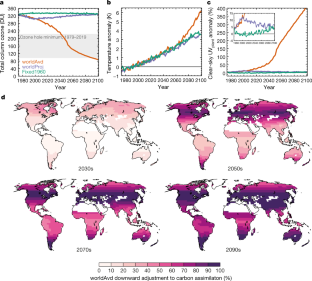
Mitigation of ozone damage to the world’s land ecosystems by source sector

Ozone depletion, ultraviolet radiation, climate change and prospects for a sustainable future

Amplified warming from physiological responses to carbon dioxide reduces the potential of vegetation for climate change mitigation

Data availability.

All relevant JULES and NIWA–UKCA model output and input data have been archived ( https://doi.org/10.5281/zenodo.4733883 ).

Code availability

The JULES code for these simulations is available on the Met Office Science Repository System (MOSRS; https://code.metoffice.gov.uk/trac/jules ; registration required) in revision 15798. Simulations were run using the Rose suite u-bb620, also available through MOSRS. The NIWA–UKCA CCM is based on the HadGEM3 climate model, which is available under licence. Please contact O.M. ([email protected]) for details.

World Meteorological Organization. Scientific Assessment of Ozone Depletion: 2018 . Report No. 58 (Global Ozone and Research Monitoring Project, 2018).

van Dijk, A. et al. Skin cancer risks avoided by the Montreal Protocol—worldwide modeling integrating coupled climate‐chemistry models with a risk model for UV. Photochem. Photobiol . 89 , 234–246 (2013).

Article   PubMed   Google Scholar  

McKenzie, R. et al. Success of Montreal Protocol demonstrated by comparing high-quality UV measurements with ‘World Avoided’ calculations from two chemistry-climate models. Sci. Rep . 9 , 12332 (2019).

Article   ADS   PubMed   PubMed Central   Google Scholar  

Ramanathan, V. Greenhouse effect due to chlorofluorocarbons: climatic implications. Science 190 , 50–52 (1975).

Article   ADS   CAS   Google Scholar  

Morgenstern, O. et al. The world avoided by the Montreal Protocol. Geophys. Res. Lett . 35 , L16811 (2008).

Article   ADS   Google Scholar  

Newman, P. A. et al. What would have happened to the ozone layer if chlorofluorocarbons (CFCs) had not been regulated? Atmos. Chem. Phys . 9 , 2113–2128 (2009).

Garcia, R. R., Kinnison, D. E. & Marsh, D. R. ‘World avoided’ simulations with the Whole Atmosphere Community Climate Model. J. Geophys. Res . 117 , D23303 (2012).

ADS   Google Scholar  

Ballaré, C. L., Caldwell, M. M., Flint, S. D., Robinson, S. A. & Bornman, J. F. Effects of solar ultraviolet radiation on terrestrial ecosystems. Patterns, mechanisms, and interactions with climate change. Photochem. Photobiol. Sci . 10 , 226–241 (2011).

Newsham, K. K. & Robinson, S. A. Responses of plants in polar regions to UVB exposure: a meta-analysis. Glob. Change Biol . 15 , 2574–2589 (2009).

Li, F.-R., Peng, S.-L., Chen, B.-M. & Hou, Y.-P. A meta-analysis of the responses of woody and herbaceous plants to elevated ultraviolet-B radiation. Acta Oecol . 36 , 1–9 (2010).

Searles, P. S., Flint, S. D. & Caldwell, M. M. A meta-analysis of plant field studies simulating stratospheric ozone depletion. Oecologia 127 , 1–10 (2001).

Article   ADS   PubMed   Google Scholar  

Fu, G. & Shen, Z.-X. Effects of enhanced UV-B radiation on plant physiology and growth on the Tibetan Plateau: a meta-analysis. Acta Physiol. Plant . 39 , 85 (2017).

Article   Google Scholar  

Lucas, R. M. et al. Human health in relation to exposure to solar ultraviolet radiation under changing stratospheric ozone and climate. Photochem. Photobiol. Sci . 18 , 641–680 (2019).

Article   CAS   PubMed   Google Scholar  

Bornman, J. F. et al. Linkages between stratospheric ozone, UV radiation and climate change and their implications for terrestrial ecosystems. Photochem. Photobiol. Sci . 18 , 681–716 (2019).

Williamson, C. E. et al. The interactive effects of stratospheric ozone depletion, UV radiation, and climate change on aquatic ecosystems. Photochem. Photobiol. Sci . 18 , 717–746 (2019).

Molina, M. J. & Rowland, F. S. Stratospheric sink for chlorofluoromethanes: chlorine atom-catalysed destruction of ozone. Nature 249 , 810–812 (1974).

Solomon, S., Garcia, R. R., Rowland, F. S. & Wuebbles, D. J. On the depletion of Antarctic ozone. Nature 321 , 755–758 (1986).

Solomon, S. Stratospheric ozone depletion: a review of concepts and history. Rev. Geophys . 37 , 275–316 (1999).

Velders, G. J. M., Andersen, S. O., Daniel, J. S., Fahey, D. W. & McFarland, M. The importance of the Montreal Protocol in protecting climate. Proc. Natl Acad. Sci. USA 104 , 4814–4819 (2007).

Article   ADS   CAS   PubMed   PubMed Central   Google Scholar  

Prather, M., Midgley, P., Rowland, F. S. & Stolarski, R. The ozone layer: the road not taken. Nature 381 , 551–554 (1996).

Wu, Y., Polvani, L. M. & Seager, R. The importance of the Montreal Protocol in protecting Earth’s hydroclimate. J. Clim . 26 , 4049–4068 (2013).

Polvani, L. M., Camargo, S. J. & Garcia, R. R. The importance of the Montreal Protocol in mitigating the potential intensity of tropical cyclones. J. Clim . 29 , 2275–2289 (2016).

Previdi, M. & Polvani, L. M. Impact of the Montreal Protocol on Antarctic surface mass balance and implications for global sea level rise. J. Clim . 30 , 7247–7253 (2017).

Chipperfield, M. P. et al. Quantifying the ozone and ultraviolet benefits already achieved by the Montreal Protocol. Nat. Commun . 6 , 7233 (2015).

Article   ADS   CAS   PubMed   Google Scholar  

Newman, P. A. & McKenzie, R. UV impacts avoided by the Montreal Protocol. Photochem. Photobiol. Sci . 10 , 1152–1160 (2011).

Neugart, S. & Schreiner, M. UVB and UVA as eustressors in horticultural and agricultural crops. Sci. Hortic . 234 , 370–381 (2018).

Article   CAS   Google Scholar  

Fiscus, E. L. & Booker, F. L. Is increased UV-B a threat to crop photosynthesis and productivity? Photosynth. Res . 43 , 81–92 (1995).

Morgenstern, O. et al. Review of the global models used within phase 1 of the Chemistry–Climate Model Initiative (CCMI). Geosci. Model Dev . 10 , 639–671 (2017).

Best, M. J. et al. The Joint UK Land Environment Simulator (JULES), model description–part 1: energy and water fluxes. Geosci. Model Dev . 4 , 677–699 (2011).

Clark, D. B. et al. The Joint UK Land Environment Simulator (JULES), model description–part 2: carbon fluxes and vegetation dynamics. Geosci. Model Dev . 4 , 701–722 (2011).

van Vuuren, D. P. et al. The representative concentration pathways: an overview. Clim. Change 109 , 5–31 (2011).

Barlow, J. et al. The future of hyperdiverse tropical ecosystems. Nature 559 , 517–526 (2018).

Collins, M. et al. in Climate Change 2013-The Physical Science Basis: Contribution of Working Group I to the Fifth Assessment Report of the Intergovernmental Panel on Climate Change (eds Stocker, T. F. et al.) 1029–1136 (Cambridge Univ. Press, 2013).

Cox, P. M., Betts, R. A., Jones, C. D., Spall, S. A. & Totterdell, I. J. Acceleration of global warming due to carbon-cycle feedbacks in a coupled climate model. Nature 408 , 184–187 (2000); erratum 408 , 750 (2000).

Heimann, M. & Reichstein, M. Terrestrial ecosystem carbon dynamics and climate feedbacks. Nature 451 , 289–292 (2008).

Caldwell, M. M. in Photophysiology, Current Topics in Photobiology and Photochemistry Vol. VI (ed. Giese, A. C.) 131–177 (Academic Press, 1971).

Caldwell, M. M., Camp, L. B., Warner, C. W. & Flint, S. D. in Stratospheric Ozone Reduction, Solar Ultraviolet Radiation and Plant Life Vol. 8 (eds Worrest, R. C. & Caldwell, M. M.) 87–111 (Springer, 1986).

Calbó, J., Pagès, D. & González, J. Empirical studies of cloud effects on UV radiation: a review. Rev. Geophys . 43 , RG2002 (2005).

Arora, V. K. et al. Carbon–concentration and carbon–climate feedbacks in CMIP5 Earth system models. J. Clim . 26 , 5289–5314 (2013).

Williamson, C. E. et al. Solar ultraviolet radiation in a changing climate. Nat. Clim. Chang . 4 , 434–441 (2014).

Rigby, M. et al. Increase in CFC-11 emissions from eastern China based on atmospheric observations. Nature 569 , 546–550 (2019).

Tilmes, S., Garcia, R. R., Kinnison, D. E., Gettelman, A. & Rasch, P. J. Impact of geoengineered aerosols on the troposphere and stratosphere. J. Geophys. Res . 114 , D12305 (2009).

NASA. Ozone Watch https://ozonewatch.gsfc.nasa.gov/meteorology/annual_data.html (2019).

Morgenstern, O. et al. Evaluation of the new UKCA climate-composition model – part 1: the stratosphere. Geosci. Model Dev . 2 , 43–57 (2009).

Hewitt, H. T. et al. Design and implementation of the infrastructure of HadGEM3: the next-generation Met Office climate modelling system. Geosci. Model Dev . 4 , 223–253 (2011).

World Meteorological Organization. Scientific Assessment of Ozone Depletion: 2010 . Report No. 52 (Global Ozone Research and Monitoring Project, 2011).

Morgenstern, O. et al. Ozone sensitivity to varying greenhouse gases and ozone-depleting substances in CCMI-1 simulations. Atmos. Chem. Phys . 18 , 1091–1114 (2018).

Edwards, J. M. & Slingo, A. Studies with a flexible new radiation code. I: choosing a configuration for a large-scale model. Q. J. R. Meteorol. Soc . 122 , 689–719 (1996).

Forster, P. M. et al. Evaluation of radiation scheme performance within chemistry climate models. J. Geophys. Res . 116 , D10302 (2011).

Lauer, A. & Hamilton, K. Simulating clouds with global climate models: a comparison of CMIP5 results with CMIP3 and satellite data. J. Clim . 26 , 3823–3845 (2013).

Dee, D. P. et al. The ERA-Interim reanalysis: configuration and performance of the data assimilation system. Q. J. R. Meteorol. Soc . 137 , 553–597 (2011).

Flint, S. D. & Caldwell, M. M. A biological spectral weighting function for ozone depletion research with higher plants. Physiol. Plant . 117 , 137–144 (2003).

Kotilainen, T., Lindfors, A., Tegelberg, R. & Aphalo, P. J. How realistically does outdoor UV-B supplementation with lamps reflect ozone depletion: an assessment of enhancement errors. Photochem. Photobiol . 87 , 174–183 (2011).

Flint, S. D., Ryel, R. J. & Caldwell, M. M. Ecosystem UV-B experiments in terrestrial communities: a review of recent findings and methodologies. Agric. For. Meteorol . 120 , 177–189 (2003).

Poulter, B. et al. Plant functional type classification for earth system models: results from the European Space Agency’s Land Cover Climate Change Initiative. Geosci. Model Dev . 8 , 2315–2328 (2015).

Harper, A. B. et al. Improved representation of plant functional types and physiology in the Joint UK Land Environment Simulator (JULES v4.2) using plant trait information. Geosci. Model Dev . 9 , 2415–2440 (2016).

Harper, A. B. et al. Vegetation distribution and terrestrial carbon cycle in a carbon cycle configuration of JULES4.6 with new plant functional types. Geosci. Model Dev . 11 , 2857–2873 (2018).

Huntingford, C. & Cox, P. M. An analogue model to derive additional climate change scenarios from existing GCM simulations. Clim. Dyn . 16 , 575–586 (2000).

Meinshausen, M. et al. The RCP greenhouse gas concentrations and their extensions from 1765 to 2300. Clim. Change 109 , 213–241 (2011).

Huntingford, C. et al. Using a GCM analogue model to investigate the potential for Amazonian forest dieback. Theor. Appl. Climatol . 78 , 177–185 (2004).

Friedlingstein, P. et al. Climate–carbon cycle feedback analysis: results from the C4MIP model intercomparison. J. Clim . 19 , 3337–3353 (2006).

Download references

Acknowledgements

P.J.Y. was supported by the UK Engineering and Physical Science Research Council (grant EP/R01860X/1), the Natural Environment Research Council (grant NE/R004927/1) and the Faculty of Science and Technology at Lancaster University. A.B.H. acknowledges funding from the UK Engineering and Physical Science Research Council (Fellowship EP/N030141/1) and the Natural Environment Research Council (grant NE/P019951/1). C.H. acknowledges a UK National Capability grant given to the UK Centre for Ecology and Hydrology. O.M. was supported by the NZ Government’s Strategic Science Investment Fund (SSIF) through the NIWA programme CACV. L.D.O. is supported by the NASA Modeling, Analysis, and Prediction programme. S.M. and R.R.G. are supported by the National Center for Atmospheric Research, which is a major facility sponsored by the US National Science Foundation under cooperative agreement number 1852977. We acknowledge the contribution of New Zealand’s national high-performance computing facilities to the results of this research, provided by the NZ eScience Infrastructure (NeSI) and funded jointly by NeSI’s collaborator institutions and through the NZ Ministry for Business, Innovation and Employment’s Research Infrastructure Programme.

Author information

Authors and affiliations.

Lancaster Environment Centre, Lancaster University, Lancaster, UK

Paul J. Young & Nigel D. Paul

Institute for Social Futures, Lancaster University, Lancaster, UK

Paul J. Young

Centre of Excellence for Environmental Data Science, Lancaster University and the UK Centre of Ecology and Hydrology, Lancaster, UK

College of Engineering, Mathematics, and Physical Sciences, University of Exeter, Exeter, UK

Anna B. Harper

Global Systems Institute, University of Exeter, Exeter, UK

UK Centre for Ecology and Hydrology, Wallingford, UK

Chris Huntingford

Centre for Global Eco-Innovation, Lancaster University, Lancaster, UK

Nigel D. Paul

National Institute of Water and Atmospheric Research, Wellington, Aotearoa New Zealand

Olaf Morgenstern

NASA Goddard Space Flight Center, Greenbelt, MD, USA

Paul A. Newman & Luke D. Oman

National Center for Atmospheric Research, Boulder, CO, USA

Sasha Madronich & Rolando R. Garcia

You can also search for this author in PubMed   Google Scholar

Contributions

P.J.Y. conceived the initial study on the basis of conversations with N.D.P. P.J.Y., A.B.H. and C.H. designed and constructed the modelling framework and the simulations, performed the analysis and, with N.D.P., wrote the manuscript. O.M., P.A.N., L.D.O., S.M. and R.R.G. provided model simulation data to run the framework and input to the parameterizations used, and contributed to writing the manuscript.

Corresponding author

Correspondence to Paul J. Young .

Ethics declarations

Competing interests.

The authors declare no competing interests.

Additional information

Peer review information Nature thanks Pedro J. Aphalo, Benjamin Felzer, Veerabhadran Ramanathan and the other, anonymous, reviewer(s) for their contribution to the peer review of this work. Peer reviewer reports are available.

Publisher’s note Springer Nature remains neutral with regard to jurisdictional claims in published maps and institutional affiliations.

Extended data figures and tables

Extended data fig. 1 effects on npp for different latitude bands..

a – c , NPP time series data from JULES, as per Fig. 2a , but for 30°–60° N ( a ), 30° S–30° N ( b ) and 55°–30° S ( c ).

Supplementary information

Peer review file, rights and permissions.

Reprints and permissions

About this article

Cite this article.

Young, P.J., Harper, A.B., Huntingford, C. et al. The Montreal Protocol protects the terrestrial carbon sink. Nature 596 , 384–388 (2021). https://doi.org/10.1038/s41586-021-03737-3

Download citation

Received : 31 July 2020

Accepted : 18 June 2021

Published : 18 August 2021

Issue Date : 19 August 2021

DOI : https://doi.org/10.1038/s41586-021-03737-3

Share this article

Anyone you share the following link with will be able to read this content:

Sorry, a shareable link is not currently available for this article.

Provided by the Springer Nature SharedIt content-sharing initiative

This article is cited by

Changes in tropospheric air quality related to the protection of stratospheric ozone in a changing climate.

• S. Madronich
• B. Sulzberger
• S. R. Wilson

Photochemical & Photobiological Sciences (2023)

Interactive effects of changes in UV radiation and climate on terrestrial ecosystems, biogeochemical cycles, and feedbacks to the climate system

• P. W. Barnes
• T. M. Robson

Stratospheric ozone, UV radiation, and climate interactions

• G. H. Bernhard
• R. L. McKenzie

The wide presence of fluorinated compounds in common chemical products and the environment: a review

• Weilan Zhang
• Yanna Liang

Environmental Science and Pollution Research (2023)

Differences in Soil Organic Carbon Accumulation After 8 Years of Biochar Application with High and Low Rates

• Xiaoyuan Zhang
• Dandan Wang

Journal of Soil Science and Plant Nutrition (2023)

By submitting a comment you agree to abide by our Terms and Community Guidelines . If you find something abusive or that does not comply with our terms or guidelines please flag it as inappropriate.

Quick links

• Explore articles by subject
• Guide to authors
• Editorial policies

Sign up for the Nature Briefing newsletter — what matters in science, free to your inbox daily.

• Search Menu
• Sign in through your institution
• Browse content in Arts and Humanities
• Browse content in Archaeology
• Anglo-Saxon and Medieval Archaeology
• Archaeological Methodology and Techniques
• Archaeology by Region
• Archaeology of Religion
• Archaeology of Trade and Exchange
• Biblical Archaeology
• Contemporary and Public Archaeology
• Environmental Archaeology
• Historical Archaeology
• History and Theory of Archaeology
• Industrial Archaeology
• Landscape Archaeology
• Mortuary Archaeology
• Prehistoric Archaeology
• Underwater Archaeology
• Zooarchaeology
• Browse content in Architecture
• Architectural Structure and Design
• History of Architecture
• Residential and Domestic Buildings
• Theory of Architecture
• Browse content in Art
• Art Subjects and Themes
• History of Art
• Industrial and Commercial Art
• Theory of Art
• Biographical Studies
• Byzantine Studies
• Browse content in Classical Studies
• Classical Literature
• Classical Reception
• Classical History
• Classical Philosophy
• Classical Mythology
• Classical Art and Architecture
• Classical Oratory and Rhetoric
• Greek and Roman Papyrology
• Greek and Roman Archaeology
• Greek and Roman Epigraphy
• Greek and Roman Law
• Late Antiquity
• Religion in the Ancient World
• Digital Humanities
• Browse content in History
• Colonialism and Imperialism
• Diplomatic History
• Environmental History
• Genealogy, Heraldry, Names, and Honours
• Genocide and Ethnic Cleansing
• Historical Geography
• History by Period
• History of Emotions
• History of Agriculture
• History of Education
• History of Gender and Sexuality
• Industrial History
• Intellectual History
• International History
• Labour History
• Legal and Constitutional History
• Local and Family History
• Maritime History
• Military History
• National Liberation and Post-Colonialism
• Oral History
• Political History
• Public History
• Regional and National History
• Revolutions and Rebellions
• Slavery and Abolition of Slavery
• Social and Cultural History
• Theory, Methods, and Historiography
• Urban History
• World History
• Browse content in Language Teaching and Learning
• Language Learning (Specific Skills)
• Language Teaching Theory and Methods
• Browse content in Linguistics
• Applied Linguistics
• Cognitive Linguistics
• Computational Linguistics
• Forensic Linguistics
• Grammar, Syntax and Morphology
• Historical and Diachronic Linguistics
• History of English
• Language Evolution
• Language Reference
• Language Variation
• Language Families
• Language Acquisition
• Lexicography
• Linguistic Anthropology
• Linguistic Theories
• Linguistic Typology
• Phonetics and Phonology
• Psycholinguistics
• Sociolinguistics
• Translation and Interpretation
• Writing Systems
• Browse content in Literature
• Bibliography
• Children's Literature Studies
• Literary Studies (Romanticism)
• Literary Studies (American)
• Literary Studies (Modernism)
• Literary Studies (Asian)
• Literary Studies (European)
• Literary Studies (Eco-criticism)
• Literary Studies - World
• Literary Studies (1500 to 1800)
• Literary Studies (19th Century)
• Literary Studies (20th Century onwards)
• Literary Studies (African American Literature)
• Literary Studies (British and Irish)
• Literary Studies (Early and Medieval)
• Literary Studies (Fiction, Novelists, and Prose Writers)
• Literary Studies (Gender Studies)
• Literary Studies (Graphic Novels)
• Literary Studies (History of the Book)
• Literary Studies (Plays and Playwrights)
• Literary Studies (Poetry and Poets)
• Literary Studies (Postcolonial Literature)
• Literary Studies (Queer Studies)
• Literary Studies (Science Fiction)
• Literary Studies (Travel Literature)
• Literary Studies (War Literature)
• Literary Studies (Women's Writing)
• Literary Theory and Cultural Studies
• Mythology and Folklore
• Shakespeare Studies and Criticism
• Browse content in Media Studies
• Browse content in Music
• Applied Music
• Dance and Music
• Ethics in Music
• Ethnomusicology
• Gender and Sexuality in Music
• Medicine and Music
• Music Cultures
• Music and Media
• Music and Culture
• Music and Religion
• Music Education and Pedagogy
• Music Theory and Analysis
• Musical Scores, Lyrics, and Libretti
• Musical Structures, Styles, and Techniques
• Musicology and Music History
• Performance Practice and Studies
• Race and Ethnicity in Music
• Sound Studies
• Browse content in Performing Arts
• Browse content in Philosophy
• Aesthetics and Philosophy of Art
• Epistemology
• Feminist Philosophy
• History of Western Philosophy
• Metaphysics
• Moral Philosophy
• Non-Western Philosophy
• Philosophy of Language
• Philosophy of Mind
• Philosophy of Perception
• Philosophy of Action
• Philosophy of Law
• Philosophy of Religion
• Philosophy of Science
• Philosophy of Mathematics and Logic
• Practical Ethics
• Social and Political Philosophy
• Browse content in Religion
• Biblical Studies
• Christianity
• East Asian Religions
• History of Religion
• Judaism and Jewish Studies
• Qumran Studies
• Religion and Education
• Religion and Health
• Religion and Politics
• Religion and Science
• Religion and Law
• Religion and Art, Literature, and Music
• Religious Studies
• Browse content in Society and Culture
• Cookery, Food, and Drink
• Cultural Studies
• Customs and Traditions
• Ethical Issues and Debates
• Hobbies, Games, Arts and Crafts
• Natural world, Country Life, and Pets
• Popular Beliefs and Controversial Knowledge
• Sports and Outdoor Recreation
• Technology and Society
• Travel and Holiday
• Visual Culture
• Browse content in Law
• Arbitration
• Browse content in Company and Commercial Law
• Commercial Law
• Company Law
• Browse content in Comparative Law
• Systems of Law
• Competition Law
• Browse content in Constitutional and Administrative Law
• Government Powers
• Judicial Review
• Local Government Law
• Military and Defence Law
• Parliamentary and Legislative Practice
• Construction Law
• Contract Law
• Browse content in Criminal Law
• Criminal Procedure
• Criminal Evidence Law
• Sentencing and Punishment
• Employment and Labour Law
• Environment and Energy Law
• Browse content in Financial Law
• Banking Law
• Insolvency Law
• History of Law
• Human Rights and Immigration
• Intellectual Property Law
• Browse content in International Law
• Private International Law and Conflict of Laws
• Public International Law
• IT and Communications Law
• Jurisprudence and Philosophy of Law
• Law and Society
• Law and Politics
• Browse content in Legal System and Practice
• Courts and Procedure
• Legal Skills and Practice
• Primary Sources of Law
• Regulation of Legal Profession
• Medical and Healthcare Law
• Browse content in Policing
• Criminal Investigation and Detection
• Police and Security Services
• Police Procedure and Law
• Police Regional Planning
• Browse content in Property Law
• Personal Property Law
• Study and Revision
• Terrorism and National Security Law
• Browse content in Trusts Law
• Wills and Probate or Succession
• Browse content in Medicine and Health
• Browse content in Allied Health Professions
• Arts Therapies
• Clinical Science
• Dietetics and Nutrition
• Occupational Therapy
• Operating Department Practice
• Physiotherapy
• Radiography
• Speech and Language Therapy
• Browse content in Anaesthetics
• General Anaesthesia
• Neuroanaesthesia
• Clinical Neuroscience
• Browse content in Clinical Medicine
• Acute Medicine
• Cardiovascular Medicine
• Clinical Genetics
• Clinical Pharmacology and Therapeutics
• Dermatology
• Endocrinology and Diabetes
• Gastroenterology
• Genito-urinary Medicine
• Geriatric Medicine
• Infectious Diseases
• Medical Toxicology
• Medical Oncology
• Pain Medicine
• Palliative Medicine
• Rehabilitation Medicine
• Respiratory Medicine and Pulmonology
• Rheumatology
• Sleep Medicine
• Sports and Exercise Medicine
• Community Medical Services
• Critical Care
• Emergency Medicine
• Forensic Medicine
• Haematology
• History of Medicine
• Browse content in Medical Skills
• Clinical Skills
• Communication Skills
• Nursing Skills
• Surgical Skills
• Medical Ethics
• Browse content in Medical Dentistry
• Oral and Maxillofacial Surgery
• Paediatric Dentistry
• Restorative Dentistry and Orthodontics
• Surgical Dentistry
• Medical Statistics and Methodology
• Browse content in Neurology
• Clinical Neurophysiology
• Neuropathology
• Nursing Studies
• Browse content in Obstetrics and Gynaecology
• Gynaecology
• Occupational Medicine
• Ophthalmology
• Otolaryngology (ENT)
• Browse content in Paediatrics
• Neonatology
• Browse content in Pathology
• Chemical Pathology
• Clinical Cytogenetics and Molecular Genetics
• Histopathology
• Medical Microbiology and Virology
• Patient Education and Information
• Browse content in Pharmacology
• Psychopharmacology
• Browse content in Popular Health
• Caring for Others
• Complementary and Alternative Medicine
• Self-help and Personal Development
• Browse content in Preclinical Medicine
• Cell Biology
• Molecular Biology and Genetics
• Reproduction, Growth and Development
• Primary Care
• Professional Development in Medicine
• Browse content in Psychiatry
• Addiction Medicine
• Child and Adolescent Psychiatry
• Forensic Psychiatry
• Learning Disabilities
• Old Age Psychiatry
• Psychotherapy
• Browse content in Public Health and Epidemiology
• Epidemiology
• Public Health
• Browse content in Radiology
• Clinical Radiology
• Interventional Radiology
• Nuclear Medicine
• Radiation Oncology
• Reproductive Medicine
• Browse content in Surgery
• Cardiothoracic Surgery
• Gastro-intestinal and Colorectal Surgery
• General Surgery
• Neurosurgery
• Paediatric Surgery
• Peri-operative Care
• Plastic and Reconstructive Surgery
• Surgical Oncology
• Transplant Surgery
• Trauma and Orthopaedic Surgery
• Vascular Surgery
• Browse content in Science and Mathematics
• Browse content in Biological Sciences
• Aquatic Biology
• Biochemistry
• Bioinformatics and Computational Biology
• Developmental Biology
• Ecology and Conservation
• Evolutionary Biology
• Genetics and Genomics
• Microbiology
• Molecular and Cell Biology
• Natural History
• Plant Sciences and Forestry
• Research Methods in Life Sciences
• Structural Biology
• Systems Biology
• Zoology and Animal Sciences
• Browse content in Chemistry
• Analytical Chemistry
• Computational Chemistry
• Crystallography
• Environmental Chemistry
• Industrial Chemistry
• Inorganic Chemistry
• Materials Chemistry
• Medicinal Chemistry
• Mineralogy and Gems
• Organic Chemistry
• Physical Chemistry
• Polymer Chemistry
• Study and Communication Skills in Chemistry
• Theoretical Chemistry
• Browse content in Computer Science
• Artificial Intelligence
• Computer Architecture and Logic Design
• Game Studies
• Human-Computer Interaction
• Mathematical Theory of Computation
• Programming Languages
• Software Engineering
• Systems Analysis and Design
• Virtual Reality
• Browse content in Computing
• Business Applications
• Computer Games
• Computer Security
• Computer Networking and Communications
• Digital Lifestyle
• Graphical and Digital Media Applications
• Operating Systems
• Browse content in Earth Sciences and Geography
• Atmospheric Sciences
• Environmental Geography
• Geology and the Lithosphere
• Maps and Map-making
• Meteorology and Climatology
• Oceanography and Hydrology
• Palaeontology
• Physical Geography and Topography
• Regional Geography
• Soil Science
• Urban Geography
• Browse content in Engineering and Technology
• Agriculture and Farming
• Biological Engineering
• Civil Engineering, Surveying, and Building
• Electronics and Communications Engineering
• Energy Technology
• Engineering (General)
• Environmental Science, Engineering, and Technology
• History of Engineering and Technology
• Mechanical Engineering and Materials
• Technology of Industrial Chemistry
• Transport Technology and Trades
• Browse content in Environmental Science
• Applied Ecology (Environmental Science)
• Conservation of the Environment (Environmental Science)
• Environmental Sustainability
• Environmentalist Thought and Ideology (Environmental Science)
• Management of Land and Natural Resources (Environmental Science)
• Natural Disasters (Environmental Science)
• Nuclear Issues (Environmental Science)
• Pollution and Threats to the Environment (Environmental Science)
• Social Impact of Environmental Issues (Environmental Science)
• History of Science and Technology
• Browse content in Materials Science
• Ceramics and Glasses
• Composite Materials
• Metals, Alloying, and Corrosion
• Nanotechnology
• Browse content in Mathematics
• Applied Mathematics
• Biomathematics and Statistics
• History of Mathematics
• Mathematical Education
• Mathematical Finance
• Mathematical Analysis
• Numerical and Computational Mathematics
• Probability and Statistics
• Pure Mathematics
• Browse content in Neuroscience
• Cognition and Behavioural Neuroscience
• Development of the Nervous System
• Disorders of the Nervous System
• History of Neuroscience
• Invertebrate Neurobiology
• Molecular and Cellular Systems
• Neuroendocrinology and Autonomic Nervous System
• Neuroscientific Techniques
• Sensory and Motor Systems
• Browse content in Physics
• Astronomy and Astrophysics
• Atomic, Molecular, and Optical Physics
• Biological and Medical Physics
• Classical Mechanics
• Computational Physics
• Condensed Matter Physics
• Electromagnetism, Optics, and Acoustics
• History of Physics
• Mathematical and Statistical Physics
• Measurement Science
• Nuclear Physics
• Particles and Fields
• Plasma Physics
• Quantum Physics
• Relativity and Gravitation
• Semiconductor and Mesoscopic Physics
• Browse content in Psychology
• Affective Sciences
• Clinical Psychology
• Cognitive Psychology
• Cognitive Neuroscience
• Criminal and Forensic Psychology
• Developmental Psychology
• Educational Psychology
• Evolutionary Psychology
• Health Psychology
• History and Systems in Psychology
• Music Psychology
• Neuropsychology
• Organizational Psychology
• Psychological Assessment and Testing
• Psychology of Human-Technology Interaction
• Psychology Professional Development and Training
• Research Methods in Psychology
• Social Psychology
• Browse content in Social Sciences
• Browse content in Anthropology
• Anthropology of Religion
• Human Evolution
• Medical Anthropology
• Physical Anthropology
• Regional Anthropology
• Social and Cultural Anthropology
• Theory and Practice of Anthropology
• Browse content in Business and Management
• Business Ethics
• Business History
• Business Strategy
• Business and Technology
• Business and Government
• Business and the Environment
• Comparative Management
• Corporate Governance
• Corporate Social Responsibility
• Entrepreneurship
• Health Management
• Human Resource Management
• Industrial and Employment Relations
• Industry Studies
• Information and Communication Technologies
• International Business
• Knowledge Management
• Management and Management Techniques
• Operations Management
• Organizational Theory and Behaviour
• Pensions and Pension Management
• Public and Nonprofit Management
• Strategic Management
• Supply Chain Management
• Browse content in Criminology and Criminal Justice
• Criminal Justice
• Criminology
• Forms of Crime
• International and Comparative Criminology
• Youth Violence and Juvenile Justice
• Development Studies
• Browse content in Economics
• Agricultural, Environmental, and Natural Resource Economics
• Asian Economics
• Behavioural Finance
• Behavioural Economics and Neuroeconomics
• Econometrics and Mathematical Economics
• Economic History
• Economic Methodology
• Economic Systems
• Economic Development and Growth
• Financial Markets
• Financial Institutions and Services
• General Economics and Teaching
• Health, Education, and Welfare
• History of Economic Thought
• International Economics
• Labour and Demographic Economics
• Law and Economics
• Macroeconomics and Monetary Economics
• Microeconomics
• Public Economics
• Urban, Rural, and Regional Economics
• Welfare Economics
• Browse content in Education
• Adult Education and Continuous Learning
• Care and Counselling of Students
• Early Childhood and Elementary Education
• Educational Equipment and Technology
• Educational Strategies and Policy
• Higher and Further Education
• Organization and Management of Education
• Philosophy and Theory of Education
• Schools Studies
• Secondary Education
• Teaching of a Specific Subject
• Teaching of Specific Groups and Special Educational Needs
• Teaching Skills and Techniques
• Browse content in Environment
• Applied Ecology (Social Science)
• Climate Change
• Conservation of the Environment (Social Science)
• Environmentalist Thought and Ideology (Social Science)
• Natural Disasters (Environment)
• Social Impact of Environmental Issues (Social Science)
• Browse content in Human Geography
• Cultural Geography
• Economic Geography
• Political Geography
• Browse content in Interdisciplinary Studies
• Communication Studies
• Museums, Libraries, and Information Sciences
• Browse content in Politics
• African Politics
• Asian Politics
• Chinese Politics
• Comparative Politics
• Conflict Politics
• Elections and Electoral Studies
• Environmental Politics
• European Union
• Foreign Policy
• Gender and Politics
• Human Rights and Politics
• Indian Politics
• International Relations
• International Organization (Politics)
• International Political Economy
• Irish Politics
• Latin American Politics
• Middle Eastern Politics
• Political Behaviour
• Political Economy
• Political Institutions
• Political Theory
• Political Methodology
• Political Communication
• Political Philosophy
• Political Sociology
• Politics and Law
• Politics of Development
• Public Policy
• Public Administration
• Quantitative Political Methodology
• Regional Political Studies
• Russian Politics
• Security Studies
• State and Local Government
• UK Politics
• US Politics
• Browse content in Regional and Area Studies
• African Studies
• Asian Studies
• East Asian Studies
• Japanese Studies
• Latin American Studies
• Middle Eastern Studies
• Native American Studies
• Scottish Studies
• Browse content in Research and Information
• Research Methods
• Browse content in Social Work
• Addictions and Substance Misuse
• Adoption and Fostering
• Care of the Elderly
• Child and Adolescent Social Work
• Couple and Family Social Work
• Direct Practice and Clinical Social Work
• Emergency Services
• Human Behaviour and the Social Environment
• International and Global Issues in Social Work
• Mental and Behavioural Health
• Social Justice and Human Rights
• Social Policy and Advocacy
• Social Work and Crime and Justice
• Social Work Macro Practice
• Social Work Practice Settings
• Social Work Research and Evidence-based Practice
• Welfare and Benefit Systems
• Browse content in Sociology
• Childhood Studies
• Community Development
• Comparative and Historical Sociology
• Economic Sociology
• Gender and Sexuality
• Gerontology and Ageing
• Health, Illness, and Medicine
• Marriage and the Family
• Migration Studies
• Occupations, Professions, and Work
• Organizations
• Population and Demography
• Race and Ethnicity
• Social Theory
• Social Movements and Social Change
• Social Research and Statistics
• Social Stratification, Inequality, and Mobility
• Sociology of Religion
• Sociology of Education
• Sport and Leisure
• Urban and Rural Studies
• Browse content in Warfare and Defence
• Defence Strategy, Planning, and Research
• Land Forces and Warfare
• Military Administration
• Military Life and Institutions
• Naval Forces and Warfare
• Other Warfare and Defence Issues
• Peace Studies and Conflict Resolution
• Weapons and Equipment

• < Previous chapter

16 Healing the Ozone Layer: The Montreal Protocol and the Lessons and Limits of a Global Governance Success Story

• Published: September 2019
• Cite Icon Cite
• Permissions Icon Permissions

The Montreal Protocol—the regime designed to protect the stratospheric ozone layer—has widely been hailed as the gold standard of global environmental governance and is one of few examples of international institutional cooperative arrangements successfully solving complex transnational problems. Although the stratospheric ozone layer still bears the impacts of ozone depleting substances (ODSs), the problem of ozone depletion is well on its way to being solved due to the protocol. This chapter examines how the protocol was designed and implemented in a way that has allowed it to successfully overcome a number of thorny challenges that most international environmental regimes must face: how to attract sufficient participation, how to promote compliance and manage non-compliance, how to strengthen commitments over time, how to neutralize or co-opt potential ‘veto players’, how to make the costs of implementation affordable, how to leverage public opinion in support of the regime’s goals, and, ultimately, how to promote the behavioural and policy changes needed to solve the problems and achieve the goals the regime was designed to solve. The chapter concludes that while some of the reasons for the Montreal Protocol’s success, such as fairly affordable, available substitutes for ODSs, are not easy to replicate, there are many other elements of this story that can be utilized when thinking about how to design solutions to other transnational environmental problems.

A condensed and thematically structured version of this same case study can be found at the Public Impact Observatory. See: http://www.centreforpublicimpact.org/case-study/the-montreal-protocol/

Introduction

The Montreal Protocol—the international regime designed to protect the stratospheric ozone layer—has widely been hailed as the gold standard of global environmental governance and is one of the few examples showing that international institutional cooperative arrangements can successfully solve complex transnational problems. Although the stratospheric ozone layer still bears the impacts of ozone depleting substances (ODSs), the problem of ozone depletion is on its way to being solved and the ‘ozone hole’ has started healing due to the protocol. What explains this success and what can we learn from it in tackling other complex global environmental problems such as climate change?

The ozone layer is crucial to protecting the earth from the sun’s ultraviolet radiation and is essential for absorbing ultraviolet B radiation, which, in large amounts, could seriously harm all plant, human, and animal life (Solomon 2008 ). In response to scientific evidence that man-made chemicals, chlorofluorocarbons (CFCs), posed a serious threat to stratospheric ozone the nations of the world first negotiated a framework convention, the 1985 Vienna Convention for the Protection of the Ozone Layer, and then, in response to new scientific evidence that confirmed the Antarctic ‘ozone hole’, added a regulatory agreement, the 1987 Montreal Protocol on Substances that Deplete the Ozone Layer. The Montreal Protocol has dramatically reduced ozone-depleting chemicals and the ozone layer has been projected to recover by the end of the century, although some recently discovered challenges may demand further amendments.

In this chapter, we examine how the Montreal Protocol was designed and implemented in a way that has allowed it to successfully overcome a number of challenges that most international environmental regimes must face: how to attract sufficient participation, how to promote compliance and manage non-compliance, how to strengthen commitments over time, how to neutralize or co-opt potential ‘veto players’, how to make the costs of implementation affordable, how to leverage public opinion in support of the regime’s goals, and, ultimately, how to promote the behavioural and policy changes needed to solve the problems and achieve the goals the regime was designed to address. We will conclude that while some of the reasons for the Montreal Protocol’s success, such as access to available and affordable ODS substitutes, are not easy to replicate, there are many other elements of this story that can be utilized when thinking about how to design solutions to other transnational environmental problems.

Assessing the Montreal Protocol

There is a strong case that the Montreal Protocol has performed well on all four dimensions of policy assessment used in this volume. To date, the protocol has been a programmatic success in achieving its stated objectives and has made progress towards achieving its overarching goals, which were to protect human health and the environment against the adverse effects of activities that deplete the ozone layer. As a result of their protocol obligations, countries have phased out 98 per cent of ODS globally compared to 1986 levels (Ministry for the Environment and Stats NZ 2017 : 46). In 2014, the US National Oceanic and Atmospheric Administration (NOAA) found that, after a peak in the year 2000, the atmospheric abundance of many ODSs had sunk under 1980 levels and predicted that the CFCs abundance would also fall below the levels of 1980 before 2050. This positive development can be connected directly to the Montreal Protocol (NOAA 2014 ). The worldwide production of ODSs has plummeted from some 1.2 million tons in 1986 to 80,000 tons in 2006 to being nearly eliminated in 2016 at 23,000 tons. Global ODS consumption has seen a similar trend dropping from 1.3 million tons in 1986 to 86,000 tons in 2006 and 22,000 tons in 2016 (UNEP Ozone Secretariat 2018 ). In fact, according to the Ozone Secretariat, in absence of the protocol, global CFC consumption would have been about 3 million tons in 2010 and would have reached 8 million tons in 2060, which would have resulted in a 50 per cent depletion of the ozone layer by 2035 (UNEP Ozone Secretariat 2018 ).

In sum, there is strong scientific evidence that the Montreal Protocol is indeed reaching the objectives it was designed to address. Achieving the objective to phase out ODSs is illustrative of its programmatic success. In addition, one of the goals of the policy, to close the ‘ozone hole’, is well on its way to be achieved. In 2018, researchers at NASA showed for the first time, through satellite observations, that the ‘ozone hole’ is recovering due to the reduction of chlorine from ODSs as a direct result of the Montreal Protocol (Strahan and Douglass 2018).

The second goal of the Montreal Protocol, improving public health by decreasing skin cancer risk, also has been deemed a success (Chipperfield et al. 2015 ). Although annual rates of new skin cancers in the USA and Europe are still increasing (CDC 2018 ; Boyle et al. 2004 ), we cannot attribute these numbers solely to the ozone layer because there are more factors than ozone depletion that affect skin cancer risk, e.g. the increased usage of tanning beds. Assessment models ran by scholars that took into account the difference between the ozone layer with and without the protocol’s regulations, estimate that roughly 2 million cases of skin cancer will be prevented annually by the year 2030 due to the Montreal Protocol (van Dijk et al. 2013). This suggests that there is already a positive public health effect due to action taken under the protocol, and this effect should increase in the future. Thus, the Montreal Protocol appears to have delivered on its goal of reducing skin cancer risks and protecting human health, adding to its programmatic success.

This evidence illustrates that the Montreal Protocol is clearly making progress in achieving its objectives to protect the ozone layer through a phase-out of ODSs. In addition to the ODS reduction achievements, the Ozone Secretariat also points to a number of other important accomplishments, including high compliance rates, the successful utilization of scientific evidence as a basis for policy decisions, the delivery of health, climate, and environmental benefits, and utilization of the financial mechanisms to support developing countries in achieving their reduction obligations (UNEP Ozone Secretariat 2015 ).

Politically the protocol has succeeded in attracting the participation and support of a broad coalition of developed and developing countries. The strong global commitment to the protocol is underscored by the fact that it has achieved universal support and has been ratified by 197 parties. Being part of the protocol had positive effects on countries’ reputation and political capital because the ozone depletion posed a risk for environment and public health that was shared globally. By implication, contributing to eliminating this risk would also provide globally shared environmental and public health benefits. The Montreal Protocol has also succeeded, after initial opposition, in winning the support of industry (Parson 1993 : 46). By providing a stable and predictable framework that allowed industry to transition away from ODSs to newer, less harmful, and affordable substitutes the protocol has been good for industry and the environment (Haq et al. 2001 : 134–5; Rae 2012 ).

In process terms, the structure and management of negotiations contributed to reaching a strong and innovative international regulatory agreement. The flexible design, system for implementation, and compliance procedures of the Montreal Protocol have created effective processes that have contributed to its success in attracting universal participation, increasing its ambition over time, and achieving stated objectives. The flexible design that operates according to the precautionary principle resulted in setting stringent ODS abatement targets before the science was conclusive and allowed ambition to be increased once the science indicated that stronger action was needed. The inclusion of trade sanctions against non-parties and the provision of financial incentives to developing countries encouraged countries to join the protocol and helped to rather quickly achieve full participation.

The protocol ensured that all parties had the financial and practical possibility to implement its required provisions, such as enacting national controls, by granting a certain degree of freedom during the process and offering financial help to developing countries. Hence, the process could be perceived by all participants as sufficiently fair and legitimate to encourage participation and compliance. The protocol’s non-compliance procedures have made it possible to utilize both positive incentives, such as funding and technical assistance, as well as the threat to cut off funding or enact sanctions to encourage adherence with its obligations. Not only have the initially agreed upon ODSs been successfully phased out, the protocol, aided by provisions for regular meetings and scheduled expert assessments and treaty reviews, has also undergone several amendments which added new substances to be phased out over time. The implementation of these amendments is another dimension of the procedural success of the policy.

In terms of endurance , the protocol has repeatedly succeeded in adapting and updating its objectives and instruments. To remain effective over time, environmental regimes must be able to adjust and adapt to changing circumstances that occur after the initial agreement. The Montreal Protocol has proven to be adept at responding to new information and challenges by strengthening its provisions (Young 2011 ). Annual meetings combined with periodic scientific assessments and treaty reviews have facilitated a process that has allowed the Montreal Protocol to update its targets and increase its ambition while maintaining political support among its members. The protocol’s Meeting of the Parties (MOP) has acted repeatedly to accelerate phase-out schedules for individual ODSs already covered and by adding additional chemicals to the list of those covered under the terms of the agreement as soon as more ambitious goals became economically and politically feasible (Andersen and Sarma 2002 ; Parson 2003 ). Its control provisions were strengthened through five amendments, which accelerated phase-outs and added additional substances, adopted in London (1990), Copenhagen (1992), Montreal (1997), Beijing (1999), and Kigali (2016).

Adding new families of chemicals to the list of those scheduled for phase-out under the Montreal Protocol requires a decision on the part of the MOP and acceptance on the part of member states. This stringent requirement has not been an obstacle to strengthening commitments. Moreover, the initial success of the agreement appears to have shaped virtuous cycles that have lowered the cost of compliance through institutionalized deliberation and adjustment routines during the MOPs. The Montreal Protocol now covers some 100 hazardous chemicals. Interestingly, some of the ODSs are greenhouse gases (GHG) that also contribute to climate change and the implementation of and compliance to the Montreal Protocol was so successful that research found the Montreal Protocol to have had more benefits for climate change mitigation than the Kyoto Protocol (Velders et al. 2007 ). It has been estimated, for example, that the total climate change mitigation through GHG reduction provided by the Montreal Protocol was ten to twenty times more effective than the reduction from the Kyoto Protocol’s first commitment period (Xu et al. 2013 ). It has also been claimed that a reduction of hydrofluorocarbons (HFCs) through the Montreal Protocol could prevent up to 0.5°C temperature increase by 2100 through substantial GHG emissions reduction (Zaelke et al. 2018 ). HFCs, which had not been addressed in the protocol previously, have been taken up under the latest developments of the MOP. An amendment to phase down HFCs was adopted in 2016 in Kigali, Rwanda (Bergeson 2017 ). The ratification of the Kigali Amendment by the member states is currently ongoing and it will enter into force in 2019 (European Commission 2017 ). By August 2018, 42 out of 197 member states had accepted or ratified the amendment.

The Challenge: Healing and Protecting a Global Open Access Resource

Solving vexing transnational problems such as stratospheric ozone depletion requires states to agree to the nature of the problem, negotiate an agreement to solve the problem, and then make the agreement work. Past experience and research on international cooperation and efficacy of global institutions demonstrates this is difficult to do effectively for a variety of reasons (Miles et al. 2002 ; Breitmeier et al. 2006 ; Young 2011 ). There is the sheer complexity of many transnational issues. Multilateral negotiations on issues such as ozone depletion or climate change often involve over 190 countries and touch on a wide range of issues in multiple policy areas. And then there is the difficulty of agreeing to a negotiating agenda (Young 1991 ): even when most states agree that an issue is important, they often have conflicting views on how the problem should be framed and which solutions should be pursued. Also, there are the various configurations of interests among the parties and the challenges this presents to burden sharing. Determining what is fair can be difficult to agree on and there are often multiple views regarding what is equitable (Keohane and Oppenheimer 2016 ). Veto players and public opinion can be complicating factors to reaching an agreement and then making it work once agreed. The difficulties of cooperation are also compounded by multiple levels of uncertainty. Actors don’t know at the outset whether proposed solutions will work, whether the costs of cooperation will be worth the benefits, nor whether other states will actually honour the commitments they make. Finally, once an agreement is reached, if it is to succeed it must attract a sufficient number of key states to participate, states must honour the commitments they have made and comply with the agreement’s rules (Parker 2001 , 2013 ).

The degradation of the ozone layer presented a classic common pool resource problem. Healing and protecting it from further degradation would only be successful if these underlying collective action problems could be solved on a global level: all large-scale producers and consumers of ODSs (namely CFCs and halons) needed to commit to a global cooperative solution. The atmosphere is a resource that all actors, nation-states and industries have open access to. However, to the extent it is used, i.e. through the emission of ODSs, the resource is affected and degrades continuously. In the absence of a comprehensive governance arrangement it was impossible to exclude actors from harming the ozone layer through emissions of ODSs negatively affecting global society (Epstein et al. 2014 ).

Hardin ( 1968 ) famously claimed that common pool resources of this type will always be overused and ultimately destroyed due to rivalry in consumption and the non-excludability of users. He predicted that the rational interests of involved actors to maximize their own benefits will increase the use of the resource to its destruction. To this day researchers remain sceptical as to whether the international society is capable of sidestepping this tragedy of the commons in relation to global open access resources, such as the earth’s atmosphere (Araral 2013 ).

In the case of the ozone layer, the resource’s very attributes complicate the situation and the search for a workable solution (Agrawal 2003 ; Epstein et al. 2013 ). First, the ozone layer is of global importance but effectively invisible. It is also highly mobile, implying that the emission of ODSs does not result in direct local consequences while also making it difficult for involved parties to see clear benefits for any efforts to protect and heal the ozone layer. In addition, because it takes a long time for the ozone layer to recover from the effects of ODSs, the value of potential, but distant, benefits may not motivate participating actors that desire more immediate gains (Epstein et al. 2014 ). While these resource characteristics make it potentially more difficult for countries to become motivated to engage in global cooperation and reduce emissions, they also highlight the fact that only a truly global solution (without free riders) can solve the problem, as shifting emissions to other, non-participating countries would undermine the effectiveness of any non-comprehensive regime.

The main actors involved in the process of finding a governance arrangement that would restrict the emission of ODSs for the protection of the ozone layer included nation-states and international organizations including NGOs, the European Economic Community (EEC), and, since 1972, the United Nations Environmental Programme, which went on to host many meetings and initiatives in this area. The industrial sector, notably in the form of ODS producers, also participated in the negotiations. The interests of these actors diverged widely. Some aimed for an international agreement, others felt national regulations alone would be sufficient, and some rejected the proposition that a policy to protect the ozone layer was needed at all.

Different clusters of nation-states were influential in shaping, or resisting, the negotiations to address ozone depletion. The lead states in the process, Canada, Finland, Norway, Sweden, and the United States, eventually formed a coalition to push aggressively for a global policy to reduce ODSs (Wettestad 2002 ). Many of these countries implemented national regulations comparatively early on, partly in collaboration with their industrial sectors. In the United States, for example, domestic politics, environmental concerns, and pressure from a major lawsuit had put ozone protection on the political agenda, which motivated American negotiators to push for a strong global agreement (Parson 1993 ).

Due to the economic importance of ODS chemicals, there was also a number of countries that opposed a control regime. Producer countries, represented by the European Economic Community (whose position was controlled by France, Italy, and the UK), Japan, and the Soviet Union formed one potential veto coalition. Another potential veto coalition was composed of several large developing countries, such as Brazil, China, India, and Indonesia, which wanted the option to produce ODSs in the future. Crafting an agreement that would be supported by all these factions was a tall order. UNEP and its Executive Director, Mostafa Tolba, played a central role in overcoming these obstacles by repeatedly organizing international meetings and providing a forum for negotiations. As we will discuss, Tolba’s leadership was instrumental in helping the various countries reach consensus through informal deliberations in the final stages of negotiations (Andersen and Sarma 2002 ).

The Road to Montreal

The role of scientific evidence.

Concerns about the potential depletion of the ozone layer by human activities were first raised in the early 1970s in relation to supersonic transport. Although initial scientific studies on stratospheric chlorine in Europe and the United States did not arrive at definitive conclusions, they attracted public attention and a policy debate ensued over ozone. One of the controversies and disagreements between actors regarded how much scientific certainty was needed to justify policy action to protect the ozone layer (Parson 2003 ). In the following years, attention shifted from supersonic transport to the role of CFCs and their potential negative impact on the ozone layer. Early studies, such as Molina and Rowland’s ( 1974 ) discovery of the effect of ODSs on the ozone layer, found that ozone was negatively affected by CFCs in the stratosphere, but did not quantify or predict the loss in ozone yet. This research prompted a rapid increase in scientific attention and spurred policy responses in Canada, the European Economic Community, Sweden, and the United States to restrict the use of CFCs, mainly in aerosols (Andersen and Sarma 2002 ; Parson 2003 ). Between 1978 and the final negotiations that led to the Montreal Protocol, the scientific evidence and predictions of ozone depletion varied significantly. Predicted ozone layer depletion ranged from 15 per cent in 1978 to 3–5 per cent in 1982.

Scientific knowledge can be an important factor in informing policy-makers about the severity of an emerging problem and contributing the needed pressure to overcome collective action problems (Epstein et al. 2014 ). However, before a firm scientific consensus is reached, users of a common pool resource will often resist regulation and offer competing interpretations of uncertain knowledge (Stern 2011 ). This was certainly the case in the debate over ozone protection and made the establishment of international controls extremely difficult. The variation in scientific estimates regarding potential depletion allowed several countries to reject the necessity of an international policy regulating ODS use. For example, the United Kingdom was sceptical whether regulation over a longer period would be necessary as ozone layer depletion estimates had been reduced between 1978 and 1982. Japan also repeatedly rejected any proposal to protect the ozone layer until further scientific evidence had been compiled (Andersen and Sarma 2002 ).

A breakthrough in the public debate and in the negotiations was achieved when research provided additional hard evidence that ozone depletion was a threat to the environment and public health. In 1985, the scientific discovery of the so-called ‘ozone hole’ demonstrated that the loss of ozone was much larger than could be accounted for with existing scientific models (Farman et al. 1985 ; Solomon et al. 1986 ). This discovery served as a dramatic focusing event and the resulting increase in global public attention to the problem of ozone depletion created a sense of urgency about the need for a robust global policy solution.

Support among the General Public and Industry

In addition to key nation-states and environmental NGOs, the coalition that formed around what would eventually become the Montreal Protocol also included other actors, such as specific industrial producers of ODSs, which helped to create broad public legitimacy for the agreement. In the case of ozone depletion, most of the industrial sector opposed CFC controls initially, but after 1986 industries themselves started to call for controls. When one of the leading CFC producers, the US chemical giant DuPont (25 per cent global market share in the mid-1980s), decided to support the phasing out of many chlorofluorocarbons and halons this made a big difference in reaching an agreement and to later efforts to accelerate phase-out schedules under the protocol (Parson 1993 ).

In addition, increasing scientific evidence and the discovery of the ‘ozone hole’ created an international public discourse on the issue and how to address it. Already in the late 1970s, researchers provided evidence that ‘a decline of ozone by 1 per cent would ultimately lead to a 4 per cent increase in skin cancer incidence’ (Andersen and Sarma 2002 : 49). In combination with the detection of a hole in the ozone layer, the connection between a damaged ozone layer and increased risk for skin cancer sparked international debate. Ozone depletion became framed as a matter of public health (Armstrong 1994 ; Martens 1998 ). Fears for a dramatic rise in the incidence of melanomas and glaucoma connected to increased exposure to solar radiation as a result of the thinning of the ozone layer were an important factor that created public support for an agreement to protect and heal the ozone layer. Ultimately, the damaged ozone layer became a ‘hot crisis’ (Ungar 1998 : 510) in the media and among the general public. This upped the ante for governments. Signing up to the protocol morphed from a political liability (opposed by big corporate interests) into a political asset (now supported by important segments of industry, research, the healthcare sector, and the public at large), thus lowering the threshold for doing so and locking in the commitment once it had been made (Patashnik 2008).

The Protocol Design and Negotiation Process

Sweden, Finland, and Norway took a prominent role in the early negotiations and drafted the Nordic Proposal that aimed at eliminating the use of certain CFCs in non-essential aerosols in 1983. This first proposal was the draft which would be developed into the Montreal Protocol over the following four years. The proposal met with both support (Denmark, United States, and Australia) and opposition (Japan and United Kingdom). In 1985, twenty countries and the EEC signed the Vienna Convention, the first international agreement on the protection of the ozone layer. But the framework refrained from imposing any reduction obligations on the parties and instead served the purpose of providing monitoring and data exchanges regarding the ozone layer (Skjaerseth 1992). Article 2b laid out future efforts to be taken by parties of the convention, which consisted of cooperation to achieve legislative and administrative measures to protect and heal the ozone layer (Andersen and Sarma 2002 ).

In the meantime, the Nordic countries had formed the Toronto Group together with Canada and the United States to draft a new proposal which suggested a reduction of the total CFC use in non-essential aerosols. The proposal was met with criticism from the EEC, which countered the draft with a suggestion to not restrict regulations on aerosols and instead regulate the total use and production of specific CFCs. A debate emerged between the EEC and the Toronto Group on which measures were appropriate, during which both parties accused each other’s proposals of failing to solve the actual problem of ozone depletion. By March 1985, the situation around these different approaches had not improved. Negotiations on the proposal had not progressed significantly and ‘[d]espite many attempts to take at least a first step to control CFCs, the governments failed to agree on anything concrete’ (Andersen and Sarma 2002 : 64).

The impasse had to be broken. The various camps jockeyed for position and in the following two years, a number of additional proposals were drafted by the EEC, Canada, the United States, and the Soviet Union. The EEC advocated cutting the total production of CFCs by 20 per cent. Canada suggested a global ODS emissions limit that would be allocated proportionally to countries depending on their population and gross national product. The United States suggested a freeze on consumption instead of production of CFCs, followed by a phased reduction of 95 per cent (Parson 1993 ). This proposal was supported by the Nordic countries and Switzerland. The Soviet Union suggested controlling the production of certain CFCs and freezing CFC production no earlier than in the year 2000 (Andersen and Sarma 2002 ).

A breakthrough in the negotiations was reached in 1987. One of the main drivers to reach a consensus was Mostafa Tolba, the then Executive Director of UNEP. He was largely responsible for a proposal draft in 1987 that summarized control measures without demanding commitment from parties. Tolba emphasized the importance of informal consultations, which he used to work up a draft proposal, as he found that during informal discussions representatives were more willing to rethink the positions of their governments. Emerging interpersonal respect and trust among representatives over time also made negotiations easier (Andersen and Sarma 2002 ).

Following Tolba’s draft proposal, more than fifty countries, multiple industry organizations, environmental NGOs, the UN, and a host of other actors took part in the final, intense, negotiations in 1987 which concluded with an agreement. Compromises were reached, for example, to make compliance with the agreement easier for countries where future CFC production had already been planned, such as the Soviet Union, Japan, and Luxembourg. Five CFCs and three halons fell under the agreement in the Montreal Protocol. The decision to focus on the production and consumption of chemicals instead of their use in different sectors made it possible for actors such as Japan to find alternatives for their most commonly used ODSs while reducing other gases.

The Montreal Protocol sought to achieve a reduction of both production and consumption by 50 per cent of the aforementioned ODSs. In 1990, this objective was upgraded to achieving a total phase-out of these ODSs by the year 2000. The protocol furthermore offered special conditions to developing countries in order to not harm progress in their development. The repeated international negotiations, debates on various drafts for a proposal, and the compromises in the final agreement to accommodate the specific needs and interests of particular countries can be assessed as a successful policy process (Andersen and Sarma 2002 ). One year after the protocol’s entry in force, in 1990, it had been signed by fifty-eight parties that accounted for 90 per cent of the global CFC and halon production and consumption. Over time, additional countries joined and at present the Montreal Protocol has achieved the universal ratification of 197 parties.

A crucial aspect of the Montreal Protocol was its success in overcoming collective action problems. Widespread participation was vital, because if the agreement was to work no substantial consumers or producers of ODSs could remain outside the agreement. To prevent the relocation of production facilities to countries that did not join the protocol and to create an incentive for participation, the deal included trade provisions. These provisions restricted trade in CFCs and ODSs with non-parties (Wettestad 2002 ). There was in-built momentum for change (Patashnik 2008): once the main producing countries joined the protocol, it was only a matter of time before all countries had to join or risk not having access to key chemicals. In 1990, the parties also decided to establish a Multilateral Fund to encourage developing countries to join the process by providing them with financial and technical support to phase out their use of ODSs (Andersen and Sarma 2002 ).

How the Protocol Gained Its Strength

The Montreal Protocol would not be a true success story without key elements that facilitated its implementation and earned it widespread legitimacy for its policy obligations. First, universal ratification has prevented free riding. Second, high levels of compliance with the phase-out obligations have been achieved by virtually all member states. ODSs (CFCs, halons, carbon tetrachloride, methyl chloroform, and clorobromomethane) reached a 98 per cent phase-out by 2010 (which was the scheduled goal); the remaining 2 per cent are hydrochlorofluorocarbons (HCFCs). For HCFCs, the current goal is to achieve phase-out by 2020, which is an acceleration of the previous deadline of 2030 (UNEP Ozone Secretariat 2015 ).

Coping with Compliance Challenges and Costs

Compliance has been described as the Achilles’ heel of international environmental regimes (Young 2011 ). Those who are opposed to the creation of a regime, or participation in one, often cite the high costs involved with implementation to justify their opposition. Technological innovation can often provide a solution. Once a regime is in place and those actors involved in implementation begin to give attention to how to do so efficiently, innovations can emerge that make compliance less costly than initially expected. The ozone regime is a good example of this (Haq et al. 2001 ). Producers found affordable alternatives for many ODSs and these replacements sometimes turned out to be less expensive than the original chemicals. The efficiencies that were realized in the initial implementation of the protocol have paved the way to making it easier to strengthen commitments, even those that were the subject of contentious bargaining at the outset.

Research on environmental cooperation has emphasized the importance of monitoring and enforcement mechanisms as essential attributes to promote compliance with agreements that govern common pool resources, such as the atmosphere (Ostrom 1990 ; Stern 2011 ). In addition, procedures to facilitate communication and deliberation among the partners of common pool resource governance arrangements increase the likelihood of overcoming collective action problems and preventing the free riding of actors who might attempt to use the resource without complying with the agreed upon rules (Ostrom 1990 , 2010 ). These basic assumptions can also be found in relation to research on international regimes, which has highlighted the importance of an institutional design that includes both management and enforcement features to help encourage compliance (Parker 2001 ).

The ‘management’ approach has stressed the importance of transparency, dialogue among the agreement’s parties, dispute resolution procedures, and technical and financial assistance to promote compliance. The ‘enforcement’ approach has stressed monitoring activities in conjunction with potent sanctions. Overall, the management approach has been found to maximize compliance better in some settings than enforcement, even in regulatory regimes (Chayes and Chayes 1995 ; Young 2011 ). Ideally, to get the best of both worlds, multilateral agreements should be equipped with mechanisms that provide incentives (resource carrots) for compliance while applying strong sanctions (costly sticks) for non-compliance (Parker 2011 ).

A study of the Montreal Protocol’s non-compliance procedures found that its implementation committee was most effective when the management and enforcement approaches to compliance were blended (Victor 1998 ). ‘Management avoids the most severe and unproductive antagonism, but the credible threat of tougher actions, including sanctions, helps ensure cooperation, especially when dealing with parties who are unswayed by management alone’ (Victor 1998 : 139). Thus, the mechanisms utilized to promote compliance with the agreement’s obligations have been effective and illustrate further why the protocol is both a procedural and programmatic success.

Assistance for Developing Countries

Making financial assistance available to member states that agreed to strengthen their commitments under the Montreal Protocol was a crucial factor that facilitated the commitment and political support of developing countries. In the case of the Montreal Protocol, financial arrangements are available to provide assistance to those willing to strengthen their commitments. In 1990, an amendment was added, which created the Montreal Protocol Multilateral Fund as a way to help developing countries (known as Art. 5 parties) to shift to non-ODSs or to pursue development without relying on ODSs. Thus, the regime fairly distributed costs and prevented developing countries being forced to act as free riders due to restricted compliance capacity. It has also increased the inclusion and participation of partners, facilitating the maintenance of the maximum winning coalitions that are generally associated with successful international environmental regimes (Young 2011 ).

Distributed Leadership

The effective exercise of different modes of leadership (Parker and Karlsson 2014 ), including scientific, political, and entrepreneurial leadership, from a number of key actors has been a crucial determinant in the Montreal Protocol’s success. Scientific leadership has been important in pinpointing the effect of ODSs on the stratosphere and in identifying the core environmental and public health issues that were at stake. Authoritative scientific reports on these threats have repeatedly provided an impetus for action for negotiators and the parties. For example, reports exposing the probable health impacts of the loss of stratospheric ozone that came out during the mid-1980s had a strong effect on the provisions that were included in the 1987 Montreal Protocol and, as new scientific evidence became available, on the subsequent amendments to the agreement that accelerated the phase-out schedules and added additional ODSs for elimination.

Political leadership was taken by a diverse group of actors at different stages. The Nordic countries, led by Sweden, were particularly influential in launching the process to negotiate an international agreement to protect the ozone layer (Parson 1993 : 37). Throughout the process, the Nordics, along with like-minded countries such as Canada, New Zealand, and Switzerland, were continuously involved in drafting proposals and coordinating diplomatic efforts to reach a deal (Wettestad 2002 : 160–1). The United States was also an important leader. In the early stages, the United States primarily provided intellectual and scientific leadership on the issue of ozone depletion. Then, starting in 1986, after domestic decisions to reduce CFC use, the United States exerted its diplomatic muscle by taking a strong leadership role in the negotiations (Parson 1993 ; Wettestad 2002 ).

Finally, entrepreneurial leadership by UNEP’s leader Tolba, as we have discussed above, proved pivotal in achieving agreement on the Montreal Protocol. In the post-creation phase, the Ozone Secretariat has assumed the entrepreneurial leadership mantle and has skilfully worked to ensure the successful implementation of the agreement and to help facilitate adjustments that have increased the agreement’s scope and ambition. It has done so by organizing informal and formal meetings of the parties, proposing draft language for treaty amendments, forming review panels, and involving itself in reporting and compliance issues (Wettestad 2002 : 162). In sum, the Ozone Secretariat’s role has contributed to the creation of positive feedback loops that have facilitated repeated adjustments in the policy demands of the protocol in a manner that enabled fair access for all parties to participate and influence the process, while at the same time helping the parties deliver on their obligations.

Lessons Learned and Future Challenges

Social science research on collective action problems and common pool resources in the 1960s and 1970s was largely occupied with pointing out the difficulty, and even impossibility, of cooperation among diverse groups of actors and predicted a tragic fate for public access resources. The negotiations, the agreement, and the implementation of the Montreal Protocol nevertheless demonstrates that it is feasible to overcome collective action problems (e.g. Hardin 1968 ; Olson 1971 )—even on a global scale, even when the resources in question are difficult to understand, and even if the measurable effects of policies enacted to address the problem have relatively long time horizons before their benefits are apparent.

The protocol effectively addresses the governance of the atmosphere as a global public access resource. The international negotiations surrounding climate change and greenhouse gas emissions must also address the governance of the atmosphere, and the Montreal Protocol provides an instructive case in point on how to overcome collective action problems, bring together heterogeneous actors to reach a common agreement, prevent free riding, and adjust to new scientific realities.

There are factors, however, that limit the Montreal Protocol’s applicability to other environmental challenges such as confronting climate change. First, the reduction of ODSs was comparatively simple; it involved controlling a set of specific industrial gases for which substitutes were available and the alternatives, which were quickly developed, also proved to be cheaper than the harmful substances they replaced. Reducing greenhouse gas emissions to address the problem of climate change is considerably more complex and will require more far-reaching societal transitions involving the energy, transport, and agricultural sectors, among others. Moreover, each sector contains powerful veto actors, such as the fossil fuel industry. Second, key countries with major ODS producing industries actively supported an agreement and provided leadership. In contrast, the international effort to address climate change has lacked leaders that are widely seen to be acting for the common good to solve the problem of global warming (Parker et al. 2015 ). Third, with regard to the problem of stratospheric ozone depletion, the issues of impact, fairness, and equity were clear and fairly easy to address. The effects of ozone depletion are spread across the globe and all countries are affected. Moreover, the normal North–South divide between the developed and developing world, which we see, for example, with climate change, has not been at play to the same extent here. The developed world is in just as much immediate risk due to ozone depletion and the Multilateral Ozone Fund can provide the capacity-building help and funding that keeps the costs of involvement for developing countries affordable (Wettestad 2002 ).

That said, there are lessons that are potentially relevant for other transnational environmental challenges, even ones for which we do not have simple technological solutions. An interesting aspect of the Montreal Protocol success story is how the accumulation of scientific evidence served as a catalyst for cooperation both for reaching a deal and for increasing ambition and strengthening commitments over time. It illustrates the importance and potential impact of scientific knowledge for forging collective solutions to environmental challenges. Regarding implementation, the Montreal Protocol provides good examples of fruitful strategies to facilitate compliance and build confidence through a calibrated combination of management and enforcement approaches. Moreover, although it will be far more difficult to accomplish for the reasons laid out above, climate change will ultimately need to be solved by finding substitutes for fossil fuels and providing financial help for the least able countries. This will not be easy and time will tell if the Paris Agreement and the Green Climate Fund are up to this epic challenge.

How then should we assess the international effort to address the challenge of ozone depletion? Has the Montreal Protocol saved the ozone layer for all time? Until recently, assessments of ozone depletion were very optimistic about healing the entire ozone layer. The 2014 scientific assessment identified a stable ozone column since the year 2000 and predicted a full recovery of the ozone layer by the end of the century (WMO et al. 2014 ). Scholars also found clear evidence that the depletion of the ozone layer would have been worse without the Montreal Protocol (Chipperfield et al. 2015 ). In addition, the latest evidence shows that the protocol has been successful in starting the healing process needed to repair the ozone hole (Strahan and Douglass 2018 ).

However, recent research has identified that the ozone column is declining again between the latitudes 60ºN and 60ºS, i.e. most of the world, where potential harm due to more intense UV radiation may be dramatic (Ball et al. 2018 ). Explanations range from an alteration of atmospheric circulation through climate change that shifts ozone, to negative effects of very short-lived chemicals found in, e.g. solvents and degreasing agents, which are not addressed by the Montreal Protocol (Hossaini et al. 2017 ; Ball et al. 2018 ). One of these damaging chemicals is even used to produce ODS replacements (Hossaini et al. 2017 ). These results, and the accompanying scientific uncertainty, require further investigation and raise questions concerning whether the overall impressive achievements of the protocol, so far, will be sufficient to repair the ozone layer as projected.

To date, the Montreal Protocol has been a programmatic, political, and procedural success that has, moreover, endured over time. It has achieved the specific objectives it set for itself by phasing out many harmful substances and it has contributed to the closing of the Antarctic ozone hole. However, although it clearly has had positive impacts on public health and in addressing ozone depletion, a complete recovery of the ozone layer has yet to be secured. Nonetheless, the Montreal Protocol’s successful track record of adjusting ambition in light of new scientific evidence, if it continues, suggests that the prospect of eventually healing the ozone layer is still within reach.

The case study outlined in this chapter is accompanied by a corresponding case study from the Centre for Public Impact’s (CPI) Public Impact Observatory—an international repository of public policies assessed for their impact using CPI’s Public Impact Fundamentals framework. CPI’s framework provides a way for those who work in or with government to assess public policies, to understand why they were successful, so key lessons can be drawn out for future policy work. The case can be easily located in the CPI repository at www.centreforpublicimpact.org/observatory .

Agrawal, A.   2003 . ‘ Sustainable Governance of Common-Pool Resources: Context, Methods, and Politics ’. Annual Review of Anthropology 32(1), 243–62.

Google Scholar

Andersen, S. O. and K. M. Sarma . 2002 . Protecting the Ozone Layer: The United Nations History (London: Earthscan).

Google Preview

Araral, E.   2013 . ‘ Ostrom, Hardin and the Commons: A Critical Appreciation and a Revisionist View ’. Environmental Science & Policy 36, 11–23.

Armstrong, B. K.   1994 . ‘ Stratospheric Ozone and Health ’. International Journal of Epidemiology 23(5), 873–85.

Ball, W. T. , J. Alsing , D. J. Mortlock , J. Staehelin , J. D. Haigh , T. Peter ,…and E. V. Rozanov . 2018 . ‘ Evidence for a Continuous Decline in Lower Stratospheric Ozone Offsetting Ozone Layer Recovery ’. Atmospheric Chemistry and Physics 18(2), 1379–94.

Bergeson, L. L.   2017 . ‘ The Montreal Protocol is Amended and Strengthened ’. Environmental Quality Management 26(3), 137–41.

Boyle, P. , J.-F. Doré , P. Autier , and U. Ringborg . 2004 . ‘ Cancer of the Skin: A Forgotten Problem in Europe ’. Annals of Oncology 15(1), 5–6.

Breitmeier, H. , O. R. Young , and M. Zürn . 2006 . Analyzing International Environmental Regimes: From Case Study to Database (Cambridge, MA: MIT Press).

CDC. 2018 . U.S. Cancer Statistics Working Group. U.S. Cancer Statistics Data Visualizations Tool, based on November 2017 submission data (1999–2015). U.S. Department of Health and Human Services, Centers for Disease Control and Prevention and National Cancer Institute. http://www.cdc.gov/cancer/dataviz .

Chayes, A. and A. H. Chayes . 1995 . The New Sovereignty: Compliance with International Regulatory Agreements (Cambridge, MA: Harvard University Press).

Chipperfield, M. P. , S. S. Dhomse , W. Feng , R. L. McKenzie , G. J. M. Velders , and J. A. Pyle . 2015 . ‘ Quantifying the Ozone and Ultraviolet Benefits Already Achieved by the Montreal Protocol ’. Nature Communications 6(1), 7233.

Epstein, G. , I. Pérez , M. Schoon , and C. L. Meek . 2014 . ‘ Governing the Invisible Commons: Ozone Regulation and the Montreal Protocol’.   International Journal of the Commons 8(2), 337–60.

Epstein, G. , J. M. Vogt , S. K. Mincey , M. Cox , and B. Fischer . 2013 . ‘ Missing Ecology: Integrating Ecological Perspectives with the Social-Ecological System Framework’.   International Journal of the Commons 7(2), 432–53.

European Commission. 2017 . ‘ EU Countries Trigger Entry into Force of Kigali Amendment to Montreal Protocol’.   https://ec.europa.eu/clima/news/eu-countries-trigger-entry-force-kigali-amendment-montreal-protocol_en .

Farman, J. C. , B. G. Gardiner , and J. D. Shanklin . 1985 . ‘ Large Losses of Total Ozone in Antarctica Reveal Seasonal ClO x /NO x Interaction ’. Nature 315(6016), 207–10.

Haq, G. , P. D. Bailey , M. J. Chadwick , J. Forrester , J. Kuylenstierna , G. Leach , D. Villagrasa , M. Fergusson , I. Skinner , and S. Oberthur . 2001 . ‘ Determining the Costs to Industry of Environmental Regulation ’. European Environment 11(3), 125–39.

Hardin, G.   1968 . ‘ The Tragedy of the Commons ’. Science 162, 1243–8.

Hossaini, R. , M. P. Chipperfield , S. A. Montzka , A. A. Leeson , S. S. Dhomse , and J. A. Pyle . 2017 . ‘ The Increasing Threat to Stratospheric Ozone from Dichloromethane ’. Nature Communications 8, 15962.

Keohane, R. O. and M. Oppenheimer . 2016 . ‘ Paris: Beyond the Climate Dead End through Pledge and Review? ’ Politics and Governance 4(3), 142–51.

Martens, W. J. M.   1998 . ‘ Health Impacts of Climate Change and Ozone Depletion: An Ecoepidemiologic Modeling Approach ’. Environmental Health Perspectives 106(1), 241–51.

Miles, E. L. , S. Andresen , E. M. Carlin , J. B. Skjærseth , A. Underdal , and J. Wettestad . 2002 . Environmental Regime Effectiveness: Confronting Theory with Evidence (Cambridge, MA: MIT Press).

Ministry for the Environment and Stats NZ. 2017. Our Atmosphere and Climate 2017 . http://www.mfe.govt.nz .

Molina, M. J. and. F. S. Rowland . 1974 . ‘ Stratospheric Sink for Chlorofluoromethanes: Chlorine Atom-Catalysed Destruction of Ozone ’. Nature 249(5460), 810–12.

NOAA. 2014. ‘Twenty Questions and Answers about the Ozone Layer: 2014 Update’. https://www.esrl.noaa.gov/csd/assessments/ozone/2014/twentyquestions/intro.html .

Olson, M.   1971 . The Logic of Collective Action: Public Goods and the Theory of Groups , 2nd edition (Cambridge, MA: Harvard University Press).

Ostrom, E.   1990 . Governing the Commons: The Evolution of Institutions for Collective Action (Cambridge: Cambridge University Press).

Ostrom, E.   2010 . ‘Polycentric Systems for Coping with Collective Action and Global Environmental Change ’. Global Environmental Change 20, 550–7.

Parker, C. F.   2001 . Controlling Weapons of Mass Destruction: An Evaluation of International Security Regime Significance . Acta Universitatis Upsaliensis. Skrifter utgivna av statsvetenskapliga föreningen i Uppsala, 147.

Parker, C. F.   2011 . ‘Compliance’. In B. Badie , D. Berg-Schlosser , and L. Morlino (eds), International Encyclopedia of Political Science (London: Sage Publications), pp. 367–70.

Parker, C. F.   2013 . ‘Agents, Structures and International Regime Significance’. In F. Bynander and S. Guzzini (eds), Rethinking Foreign Policy (London: Routledge), pp. 95–106.

Parker, C. F. and   C. Karlsson . 2014 . ‘Leadership and International Cooperation’. In   P. ‘t Hart and R. Rhodes (eds), The Oxford Handbook of Political Leadership (Oxford: Oxford University Press), pp. 580–94.

Parker, C. F. , C. Karlsson , and M. Hjerpe . 2015 . ‘ Climate Change Leaders and Followers: Leadership Recognition and Selection in the UNFCCC Negotiations ’. International Relations 29(4), 434–54.

Parson, E. A.   1993 . ‘Protecting the Ozone Layer’. In P. M. Haas , R. O. Keohane , and M. A. Levy (eds), Institutions for the Earth (Cambridge, MA: MIT Press), pp. 27–73.

Parson, E. A.   2003 . Protecting the Ozone Layer: Science and Strategy (Oxford: Oxford University Press).

Patashnik, E. M.   2008 . Reforms at Risk: What Happens after Major Policy Changes Are Enacted (Princeton, NJ: Princeton University Press).

Rae, I.   2012 . ‘ Saving the Ozone Layer: Why the Montreal Protocol Worked ’. The Conversation . https://theconversation.com/saving-the-ozone-layer-why-the-montreal-protocol-worked-9249 .

Skjærseth, J. B.   1992 . ‘ The “Successful” Ozone-Layer Negotiations: Are There Any Lessons to Be Learned? ’ Global Environmental Change 2(4), 292–300.

Solomon, K. R.   2008 . ‘ Effects of Ozone Depletion and UV-B Radiation on Humans and the Environment ’. Atmosphere-Ocean 46(1), 185–202.

Solomon, S. , R. R. Garcia , F. S. Rowland , and D. J. Wuebbles . 1986 . ‘ On the Depletion of Antarctic Ozone ’. Nature 321(6072), 755–8.

Stern, P. C.   2011 . ‘ Design Principles for Global Commons: Natural Resources and Emerging Technologies ’. International Journal of the Commons 5(2), 213–32.

Strahan, S. E. and A. R. Douglass . 2018 . ‘ Decline in Antarctic Ozone Depletion and Lower Stratospheric Chlorine Determined from Aura Microwave Limb Sounder Observations ’. Geophysical Research Letters 45(1), 382–90.

UNEP Ozone Secretariat. 2015 . ‘ Montreal Protocol—Achievements to Date and Challenges Ahead ’. http://42functions.net/en/MP_achievements_challenges.php .

UNEP Ozone Secretariat . 2018 . Ozone Secretariat. Data Access Centre. http://ozone.unep.org/en/data-reporting/data-centre .

Ungar, S.   1998 . ‘ Bringing the Issue Back In: Comparing the Marketability of the Ozone Hole and Global Warming ’. Social Problems 45(4), 510–27.

van Dijk, A. , H. Slaper , P. N. den Outer , O. Morgenstern , P. Braesicke , J. A. Pyle ,…and A. F. Bais . 2013 . ‘ Skin Cancer Risks Avoided by the Montreal Protocol: Worldwide Modeling Integrating Coupled Climate-Chemistry Models with a Risk Model for UV ’. Photochemistry and Photobiology 89(1), 234–46.

Velders, G. J. M. , S. O. Andersen , J. S. Daniel , D. W. Fahey , and M. McFarland , 2007 . ‘ The Importance of the Montreal Protocol in Protecting Climate ’. Proceedings of the National Academy of Sciences of the United States of America 104(12), 4814–19.

Victor, D. G.   1998 . ‘The Operation and Effectiveness of the Montreal Protocol’s Non-Compliance Procedure’. In D. Victor , K. Raustiala , and E.B. Skolnikoff (eds), The Implementation and Effectiveness of International Environmental Commitments: Theory and Practice (Cambridge, MA: MIT Press), pp. 137–76.

Wettestad, J.   2002 . ‘The Vienna Convention and Montreal Protocol on Ozone-Layer Depletion’. In E. L. Miles , S. Andresen , E. M. Carlin , J. B. Skjærseth , A. Underdal , and J. Wettestad (eds), Environmental Regime Effectiveness: Confronting Theory with Evidence (Cambridge, MA: MIT Press), pp. 149–70.

WMO, UNEP, NOAA, NASA, and European Commission. 2014 . Assessment for Decision-Makers: Scientific Assessment of Ozone Depletion: 2014 . WMO Global Ozone Research and Monitoring Project—Report No. 56. https://www.esrl.noaa.gov/csd/assessments/ozone/2014/assessment_for_decision-makers.pdf .

Xu, Y. , D. Zaelke , G. J. M. Velders , and V. Ramanathan . 2013 . ‘ Geoscientific Instrumentation Methods and Data Systems: The Role of HFCs in Mitigating 21st Century Climate Change ’. Atmospheric Chemistry and Physics 13, 6083–9.

Young, O. R.   1991 . ‘ Political Leadership and Regime Formation: On the Development of Institutions in International Society ’. International Organization 45(3), 281–309.

Young, O. R.   2011 . ‘ Effectiveness of International Environmental Regimes: Existing Knowledge, Cutting-Edge Themes, and Research Strategies ’. Proceedings of the National Academy of Sciences of the United States of America 108(50), 19853–60.

Zaelke, D. , N. Borgford-Parnell , S. O. Andersen , K. Campbell , X. Sun , D. Clare , C. Phillips , S. Herschmann , Y. P. Ling , A. Milgroom , and N. J. Sherman . 2018 . ‘ Primer on HFCs’.   Institute for Governance & Sustainable Development Working Paper . http://www.igsd.org/wp-content/uploads/2018/01/HFC-Primer-v11Jan18.pdf .

• About Oxford Academic
• Publish journals with us
• University press partners
• What we publish
• New features  
• Open access
• Institutional account management
• Rights and permissions
• Get help with access
• Accessibility
• Advertising
• Media enquiries
• Oxford University Press
• Oxford Languages
• University of Oxford

Oxford University Press is a department of the University of Oxford. It furthers the University's objective of excellence in research, scholarship, and education by publishing worldwide

• Copyright © 2024 Oxford University Press
• Cookie settings
• Cookie policy
• Privacy policy
• Legal notice

This Feature Is Available To Subscribers Only

Sign In or Create an Account

This PDF is available to Subscribers Only

For full access to this pdf, sign in to an existing account, or purchase an annual subscription.

Without the Ozone Treaty You’d Get Sunburned in 5 Minutes

Turning 30 this month, the Montreal Protocol was a landmark environmental success that serves as a model for addressing other problems, although it also has some unfinished business.

Thirty years ago this month the U.S. and other industrialized countries signed the Montreal Protocol on Substances that Deplete the Ozone Layer . It was a “milestone for all people and our planet,” said UN Secretary-General António Guterres, who highlighted the positive impacts of the Montreal Protocol on human health, poverty eradication, climate change, and protecting the food chain at an anniversary celebration.

The Earth’s ozone layer would have collapsed by 2050 with catastrophic consequences without the Montreal Protocol, studies have shown. In the world we avoided thanks to the Protocol the UV Index measure during a Washington, DC or Los Angles mid-summer day would be at least 30 by 2070 . Anything over 11 is considered extreme. There would have been an additional 280 million cases of skin cancer, 1.5 million skin cancer deaths, and 45 million cataracts in the United States, according to the U.S. EPA.

Further, climate change would have been far worse by mid-century because the chemicals that “eat” ozone are also super-greenhouse gases, thousands of times more potent than CO2. And that would have meant the potential intensity of hurricanes and cyclones would have increased three times, another stud y found.

The combined impacts of UV levels that could literally burn skin in five minutes and hotter, stormier weather is something no one would want to live in or wish for their grandchildren, said Rolando Garcia, a senior scientist at the National Center for Atmospheric Research (NCAR) in Boulder, Colorado.

Our global climate would be at least 25 per cent hotter today without the Protocol, said Garcia, a co-author of two world-avoided studies. That additional heat energy would have provided “fuel“ for today’s extreme weather events like hurricanes , floods , and droughts . By 2070 the world would have been 4.5 degrees F (2.5 degrees Celsius) hotter, a level most experts agree is disastrously high.

“In 1987 I don’t think anyone knew about the full climate implications,” said Garcia. “The Protocol saved our bacon a little bit.”

For Hungry Minds

Ozone politics.

The ozone layer acts like a shield reducing the amount of the sun's ultraviolet (UV) radiation to safer levels. By the late 1970s scientists proved chemicals used in fridges, air conditioners, and aerosol cans were damaging this ozone shield. But the chemical industry argued the science was uncertain, and more research was needed. Then, in 1985, a gigantic hole appeared in the ozone layer over Antarctica, allowing dangerous levels of UV radiation to reach the surface. By 1987 the Montreal Protocol was created to reduce the amounts of those chemicals.

Industry lobbied the Ronald Reagan White House and tried to get the Senate to deny ratification of the Protocol, warning of dire economic impacts resulting from a phase-down of their products.

“It was just as bad as the fossil fuel industry has been on climate change,” said David Doniger, Director, Climate and Clean Air Program at the Natural Resources Defense Council.

People bathe in the sea in southern France—but without a protective ozone layer, such activities would be much more dangerous.

And yet the U.S. was one of the first countries to ratify the Protocol and have been a leader on the revisions that sped up the phase-outs of ozone-destroying chemicals, Doniger said. Industry soon developed new products and got on board with the phase-out of the old chemicals.

You May Also Like

Another weapon to fight climate change? Put carbon back where we found it

Ground-level ozone is getting worse. Here's what it means for your health.

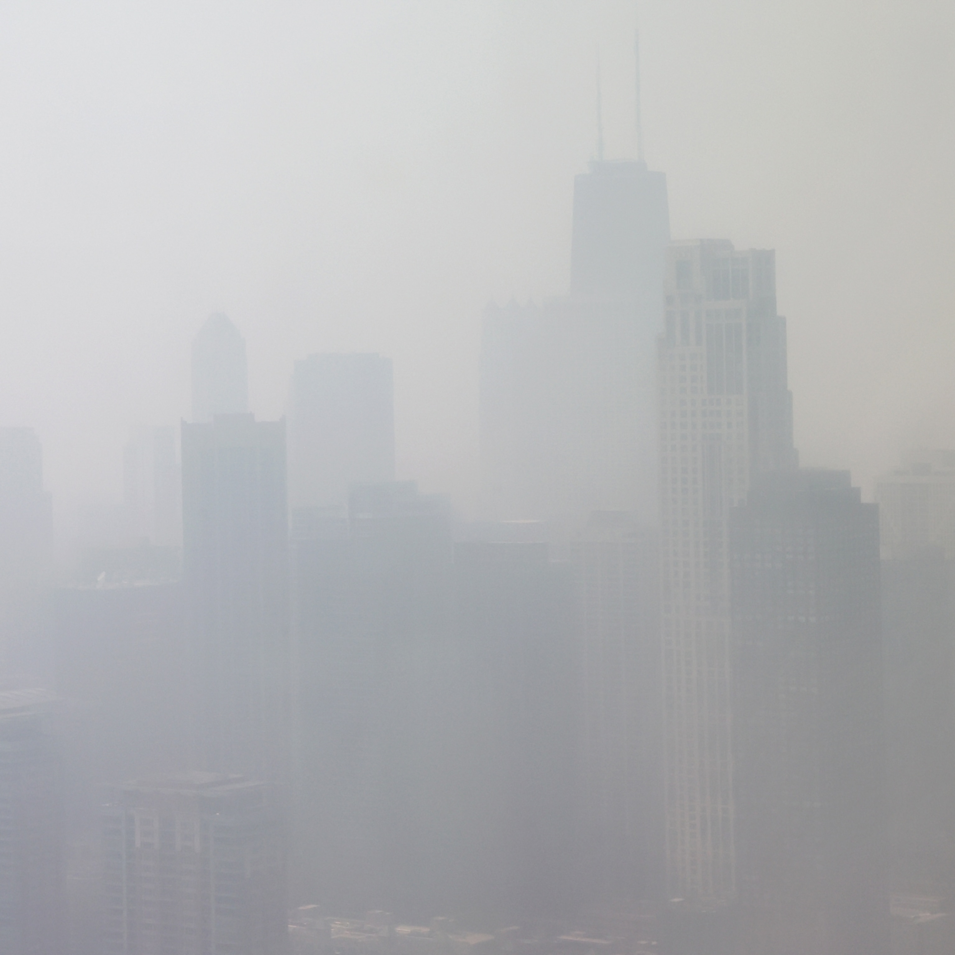
How wildfire smoke infiltrates your home—and how to get rid of it

The Protocol now has 197 countries participating and resulted in the phase-out of 99 percent of nearly 100 ozone-depleting chemicals. It’s often considered the most successful international environmental treaty in history.

"Thirty years ago the world proved it can come together and tackle a global problem with global resolve,” said Erik Solheim, head of the United Nations Environment Programme (UNEP).

“The Montreal Protocol is as necessary today as it was in the 1980s,” Solheim said.

Unfinished Business

The ozone layer is expected to recover by 2050 but the Protocol has two major pieces of unfinished business. Some countries in the developing world haven’t yet phased out ozone-damaging chemicals like R-22, a hydrochlorofluorocarbon (HCFC) found in many refrigeration and air conditioning systems. They’ll require financial support to do so, which the Protocol provides under its Multilateral Fund.

The Multilateral Fund will need to be replenished for the next three years at the upcoming Montreal Protocol conference in November. The U.S. usually provides about 20 percent of the funding, but “the Trump Administration has been completely silent on this so far,” said Doniger.

This funding is crucial to help poor countries not only eliminate the last ozone-damaging chemicals but also to leapfrog cheap replacement chemicals called hydrofluorocarbons (HFCs). While HFCs are safe for ozone, they are a powerful greenhouse gas, a thousand times worse than CO2. In 2016, after nearly ten years of negotiations, more than 150 countries agreed to reduce their use by 85 percent in the coming decades.

The use of HFCs for air conditioning and refrigeration is growing at a fast pace in developing countries, particularly China and India, Doniger said. That’s in part because climate change is producing more and longer deadly heat waves and driving up summer temperatures.

This HFC phase down is known as the Kigali Amendment to the Protocol and would have a big impact on climate change, cutting global warming up to 0.9 degrees F (0.5 degrees Celsius) by the end of the century , according to the UNEP.

That’s a big deal because even limiting global warming to under 3.6 degrees F (2 degrees Celsius) will still cut Africa’s agricultural yields by 40 percent , putting 50 percent of the continent’s population at risk of undernourishment.

“It is very much in the U.S.’s interest to help countries phase down HFCs,” says Doniger.

Related Topics

• CLIMATE CHANGE
• AIR POLLUTION

How wildfire smoke affects your body—and how you can protect yourself

Are there real ways to fight climate change? Yes.

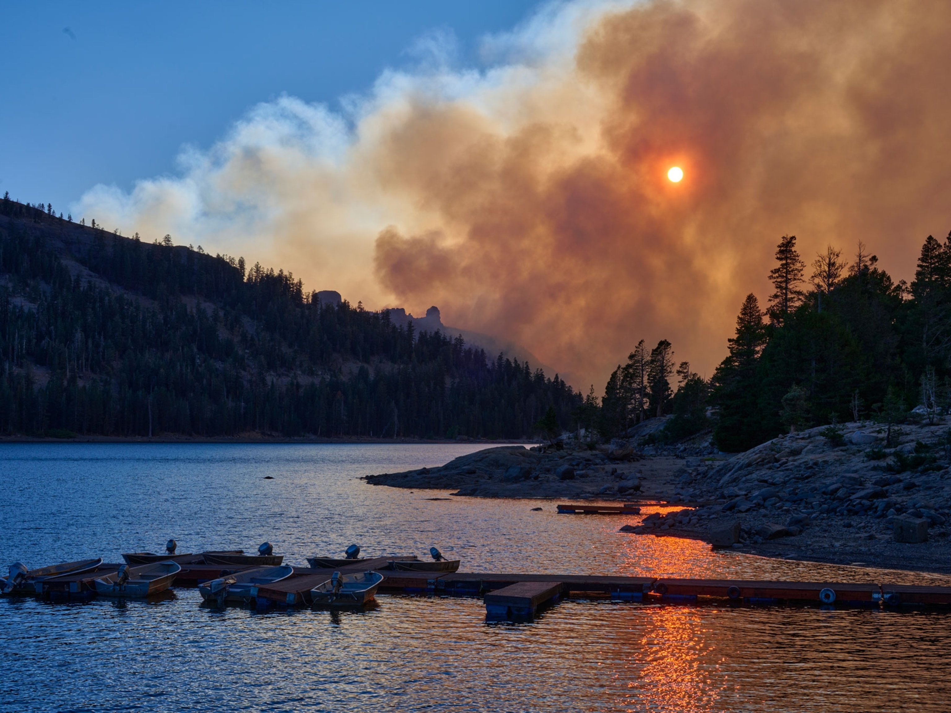
Wildfire season is getting longer—and more intense. Here's how to prepare.

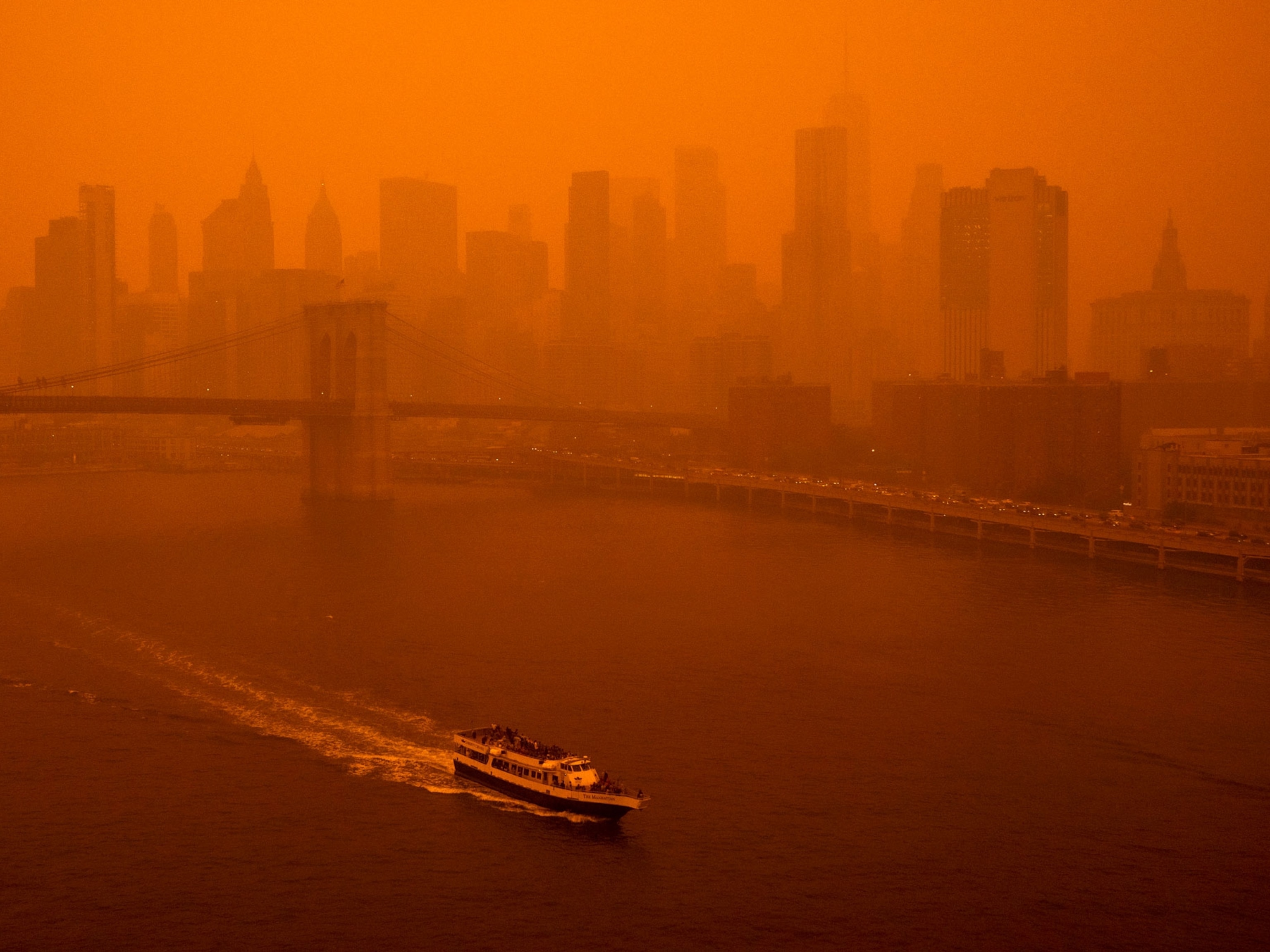
Orange skies are the future. Prepare yourself.

This African lake may literally explode—and millions are at risk

• Environment
• Paid Content
• Photography
• Perpetual Planet

History & Culture

• History & Culture
• History Magazine
• Mind, Body, Wonder
• Terms of Use
• Privacy Policy
• Your US State Privacy Rights
• Children's Online Privacy Policy
• Interest-Based Ads
• About Nielsen Measurement
• Do Not Sell or Share My Personal Information
• Nat Geo Home
• Attend a Live Event
• Book a Trip
• Inspire Your Kids
• Shop Nat Geo
• Visit the D.C. Museum
• Learn About Our Impact
• Support Our Mission
• Advertise With Us
• Customer Service
• Renew Subscription
• Manage Your Subscription
• Work at Nat Geo
• Sign Up for Our Newsletters
• Contribute to Protect the Planet

Copyright © 1996-2015 National Geographic Society Copyright © 2015-2024 National Geographic Partners, LLC. All rights reserved

Advertisement

Continuing benefits of the Montreal Protocol and protection of the stratospheric ozone layer for human health and the environment

• Original Papers
• Open access
• Published: 19 May 2024

Cite this article

You have full access to this open access article

• S. Madronich 1 , 2 ,
• G. H. Bernhard 3 ,
• P. J. Neale 4 ,
• A. Heikkilä 5 ,
• M. P. Sulbæk Andersen 6 , 7 ,
• A. L. Andrady 8 ,
• P. J. Aucamp 9 ,
• A. F. Bais 10 ,
• A. T. Banaszak 11 ,
• P. J. Barnes 12 ,
• J. F. Bornman 13 ,
• L. S. Bruckman 14 ,
• R. Busquets 15 ,
• G. Chiodo 16 ,
• D.-P. Häder 17 ,
• M. L. Hanson 18 ,
• S. Hylander 19 ,
• M. A. K. Jansen 20 ,
• G. Lingham 21 , 22 ,
• R. M. Lucas 23 ,
• R. Mackenzie Calderon 24 , 25 , 26 ,
• C. Olsen 27 ,
• R. Ossola 28 ,
• K. K. Pandey 29 ,
• I. Petropavlovskikh 30 , 31 ,
• L. E. Revell 32 ,
• L. E. Rhodes 33 , 34 ,
• S. A. Robinson 35 , 36 ,
• T. M. Robson 37 , 38 ,
• K. C. Rose 39 ,
• T. Schikowski 40 ,
• K. R. Solomon 41 ,
• B. Sulzberger 42 ,
• T. J. Wallington 43 ,
• Q.-W. Wang 44 ,
• S.-Å. Wängberg 45 ,
• C. C. White 46 ,
• S. R. Wilson 36 ,
• L. Zhu 47 &
• R. E. Neale 27 , 48  

500 Accesses

7 Altmetric

Explore all metrics

The protection of Earth’s stratospheric ozone (O 3 ) is an ongoing process under the auspices of the universally ratified Montreal Protocol and its Amendments and adjustments. A critical part of this process is the assessment of the environmental issues related to changes in O 3 . The United Nations Environment Programme’s Environmental Effects Assessment Panel provides annual scientific evaluations of some of the key issues arising in the recent collective knowledge base. This current update includes a comprehensive assessment of the incidence rates of skin cancer, cataract and other skin and eye diseases observed worldwide; the effects of UV radiation on tropospheric oxidants, and air and water quality; trends in breakdown products of fluorinated chemicals and recent information of their toxicity; and recent technological innovations of building materials for greater resistance to UV radiation. These issues span a wide range of topics, including both harmful and beneficial effects of exposure to UV radiation, and complex interactions with climate change. While the Montreal Protocol has succeeded in preventing large reductions in stratospheric O 3 , future changes may occur due to a number of natural and anthropogenic factors. Thus, frequent assessments of potential environmental impacts are essential to ensure that policies remain based on the best available scientific knowledge.

Graphical abstract

Similar content being viewed by others

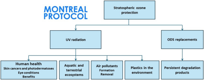
Environmental effects of stratospheric ozone depletion, UV radiation and interactions with climate change: UNEP Environmental Effects Assessment Panel, update 2019

Stratospheric Ozone Depletion

Ozone depletion, ultraviolet radiation, climate change and prospects for a sustainable future

Avoid common mistakes on your manuscript.

1 Introduction

The Earth’s stratospheric ozone (O 3 ) layer regulates the amount of ultraviolet (UV) radiation reaching the lower atmosphere and surface. Some human-made substances can destroy O 3 (ozone-depleting substances, ODSs) if emitted into the atmosphere, and therefore a phase-out of their production was agreed internationally under the 1987 Montreal Protocol. The Montreal Protocol and subsequent Amendments and adjustments have limited mid-latitude O 3 depletion to a few percent, and atmospheric concentrations of ODSs are expected to return to pre-1980 values by the middle of this century. However, larger changes in stratospheric O 3 could occur for several other reasons under different possible future scenarios. Scenarios with large greenhouse gas emissions predict increases in stratospheric O 3 , e.g., climate-dependent super-recovery with O 3 values exceeding those of 1980. Other scenarios could entail further depletion, e.g., in response to attempts to modify solar radiation reaching the Earth’s surface by injecting sulfur into the stratosphere [ 1 ].

Full implementation of the Montreal Protocol critically relies on regular scientific evaluations of the state of the ozone layer, UV radiation, and the associated effects of UV radiation on human health and ecosystems. Comprehensive Quadrennial Assessments reflect this evolving knowledge and constitute the scientific basis for any Amendments and adjustments to the Montreal Protocol; i.e., the recent assessments of ozone science [ 1 ] and effects on related environmental effects [ 2 ] (see also [ 3 , 4 , 5 , 6 , 7 , 8 , 9 , 10 , 11 ]). Annual updates assess information emerging from rapidly evolving fields and newly recognised interactions.

One important outcome of this ongoing assessment process is a move away from the notion that exposure to UV radiation is harmful in every aspect and should always be minimised. Like temperature and humidity, UV radiation is an environmental variable that increases the chemical reactivity of irradiated substances, whether these be biological tissues, materials, or atmospheric contaminants. Harmful effects—including the induction of skin cancer (Sect.  2 ) and cataracts (Sect.  3 ), formation of local photochemical smog (Sect.  5 ), and degradation of materials (Sect.  7 ) must be viewed alongside potentially beneficial effects such as production of vitamin D (Sect.  4 ), disinfection of surface waters, and regional/global destruction of air pollutants (also in Sect.  5 ). Furthermore, the phase-out of ODSs has helped to avoid additional global warming (Sect.  1.2 ). However, some of the chemicals used as replacements can degrade to compounds that are persistent in the environment (e.g., trifluoroacetic acid, TFA), requiring ongoing assessment of potential risks (Sect.  6 ).

1.1 The Montreal Protocol and global warming

Ozone-depleting substances controlled by the Montreal Protocol are also potent greenhouse gases (GHGs). The global warming potentials (GWPs) of ODSs are far greater than those of carbon dioxide (CO 2 ), e.g., Table A-5 of [ 1 ]. Hence, the increase of ODSs in the atmosphere since their invention in the 1920s and 1930s has contributed substantially to global warming. In our 2022 Quadrennial Assessment [ 2 , 5 ], we concluded that, as of 2019, the phase-out of ODSs prompted by the Montreal Protocol may have avoided warming by 0.5–1.0 °C in mid-latitude regions of the continents, and by more than 1.0 °C in the Arctic. A new study by Sigmond et al. [ 12 ] generally confirmed these earlier estimates and concluded that ODSs were responsible for 30% of global and 37% of Arctic warming between 1955 and 2005. Taking into account all GHGs (including ODSs) plus the cooling effect from the rise of anthropogenic aerosols over this period, the modelled global mean surface air temperature (GSAT) increased by 0.95 °C between 1995 and 2005, in good agreement with observations. The warming attributed to CO 2 and ODSs alone was calculated as 0.63 and 0.38 °C, respectively.

In our 2022 assessment [ 5 ], we also concluded that the uncertainty in estimating changes in GSAT from changes in ODSs is large because the depletion of stratospheric ozone caused by ODSs has a cooling effect that is not well understood [ 5 ]. New calculations by Sigmond et al. [ 12 ] using a single model confirmed that the indirect impact of ODSs on GSAT via stratospheric ozone depletion is negligible due to the relatively small radiative forcing of stratospheric ozone. While some uncertainties remain, this study adds to the emerging evidence that ODSs have played a substantial role in historical warming. By phasing out the production and consumption of ODSs, the Montreal Protocol will also play a crucial role in mitigating future climate change, including reduction of the loss of polar sea ice. Several studies find that the phase-out of ODSs will delay the appearance of an ice-free Arctic summer (defined as the first year with September sea ice extent smaller than 1 million km 2 ), by between 15 and even 40 years, depending on the model used [ 13 , 14 ].

1.2 Extremes of the UV index

Measurements from satellites suggest that the highest UV Index on Earth is about 25 and occurs at high altitudes within the tropics of the Southern Hemisphere, such as the Altiplano Region of Peru and Bolivia [ 15 ]. Recent measurements by Cordero et al. [ 16 ] using a spectroradiometer that meets the quality standards of the Network for the Detection of Atmospheric Composition Change [ 17 ] have now confirmed this value. On 22 January 2020, measurements of the UV Index performed at the Altiplano of the Atacama Desert in Chile peaked at 25.8, which can be considered the world’s highest value ever registered by a high-quality instrument. The observation occurred during partial cloudy skies when the sun was visible and clouds in the vicinity of the sun reflected additional radiation toward the instrument. This “cloud enhancement” is a well-documented effect [ 18 ]. In this particular instance, the UV Index was increased by about 30% beyond the value of 20 that would have been expected for clear skies.

These high values of the UV Index would have been greatly surpassed if the Montreal Protocol had not been implemented. According to model calculations [ 19 ], the clear-sky UV Index observed at noon during summer at mid-latitudes and the tropics would have been as high as 40 by the end of the twenty-first century in the absence of the Montreal Protocol, even before considering additional enhancements by clouds.

2 Exposure to ultraviolet radiation and the skin

Exposing the skin to UV radiation is the primary cause of skin cancer and can also lead to inflammatory skin conditions known as photodermatoses. The incidence of these conditions, particularly skin cancer, is influenced by the intensity of ambient UV radiation to which a population is exposed, so maintaining the integrity of the ozone layer is vital to avoid large increases in these medical conditions. While it is thus important to monitor trends in skin cancer, it is difficult to disentangle the effects of changes in ozone and sun exposure behaviour that have changed dramatically over the past century.

2.1 Skin cancers: malignant melanoma

2.1.1 incidence.

New population-based reports on trends in the incidence of invasive melanoma in high-risk populations, including those in Canada [ 20 ], the Netherlands [ 21 ], Lithuania [ 22 ], Minnesota (United States) [ 23 ] and some Australian states [ 24 , 25 ], generally report rising incidence over the past 2–3 decades. A concerning trend of rising incidence among children and adolescents was reported for Finland, with an average annual increase of 5.6% per year from 1990 to 2014 [ 26 ]. An increase in incidence of invasive melanoma was also reported for countries where the population is at lower inherent risk due to a high proportion of the population having darker skin types, including Columbia (2006–2015) [ 27 ], Brazil (1980–2019) [ 28 ], Jordan (2000–2016) [ 29 ], and South Korea (2008–2016) [ 30 ]. In contrast, incidence was stable in the state of South Australia between 1997 and 2016 [ 24 ], and in Hungary between 2013 and 2017 [ 31 ]. The cause of the increasing incidence, particularly in children and people who are at lower inherent risk, needs to be determined, but is likely to be driven by changes in behaviour and/or diagnostic practices rather than to any changes in ambient UV radiation.

2.1.2 Overdiagnosis as a potential contributor to increases in melanoma incidence

Melanomas that are confined to the epidermis (the top layer of the skin) at diagnosis are called melanoma in situ. Once they have invaded into the dermis they are called invasive melanomas. It is not clear how often in situ melanomas become invasive, or how long this takes. However, there is concern that a high proportion of melanomas in situ is indicative of overdiagnosis; i.e., diagnosis of a lesion that if left undetected would not have caused harm within a person’s lifetime. Potential drivers of the overdiagnosis of in situ and thin melanomas include increased awareness and attendances for skin examinations, higher rates of diagnostic biopsies and a lowering of diagnostic thresholds [ 32 ].

An analysis of long-term incidence trends (1982–2018) for in situ and invasive melanomas in three predominantly white populations with high, medium, and low melanoma rates (Queensland (Australia), United States, and Scotland, respectively) reported a much faster increase in the incidence of melanoma in situ compared to invasive melanoma in all three populations; this difference was most marked in Queensland, Australia, where opportunistic screening practices are common [ 33 ]. In the United States, the incidence of melanoma in situ is rising in all areas, whereas the incidence of invasive melanoma is stabilizing in metropolitan regions but increasing in nonmetropolitan and rural populations [ 34 ]. These trends are consistent with a pattern of overdiagnosis.

At the height of the COVID-19 pandemic, fewer notifications of skin cancers to cancer registries were reported worldwide [ 35 , 36 , 37 ]. There may be a rebound from the observed trend of a reduction in incidence in the period immediately following the pandemic, and some have suggested that delayed melanoma diagnoses may influence future mortality rates [ 38 ].

2.1.3 Mortality

Mortality rates due to skin cancer reflect both incidence and survival, so mortality rates were historically highest in regions of high incidence. The past decade has seen dramatic improvements in treatment and survival for patients with localised or metastatic disease with the use of targeted and immunotherapies, which has resulted in significant reductions in melanoma mortality over the past decade.

Analysis of recent trends in melanoma mortality in the United States showed recent stabilisation in mortality rates. Rates increased between 1975 and 1988 at a rate of 1.7% per year, stabilised between 1988 and 2013, and then decreased at a rate of 6.3% per year to 2017 [ 39 ]. Stabilising or declining mortality rates were also reported for Canada [ 20 ], Columbia [ 27 ] and the Australian state of New South Wales for all age groups under 60 years [ 25 ].

Other country-specific reports of long-term trends (e.g., decadal) in melanoma mortality generally show overall increases in mortality in recent decades, including for Italy [ 40 ], Poland [ 41 ] and Lithuania [ 22 ]. A study of trends in melanoma mortality in 28 European countries (25 member states and Norway, Russia and Switzerland) covering 6 decades (1960–2020) reported diverging trends according to age. For men and women aged 45–74 years the age-standardised melanoma mortality rate decreased in 15 countries and increased in 7. For those aged 75 years and older, mortality increased for men in all 28 countries, and for women in all except Hungary and Portugal [ 42 ]. The mortality rate was consistently higher among men compared with women and was highest in the Nordic countries. Geographic differences in mortality rates in the future will likely reflect heterogeneity in the timing of introduction and uptake of advanced new treatments across countries.

2.2 Skin cancers: keratinocyte cancers

2.2.1 incidence.

Recent reports confirm that the incidence of keratinocyte cancers continues to increase, driven largely by increases in older age groups who were not exposed to sun protection messages until later in life. The incidence of squamous cutaneous carcinoma (SCC) increased between 1990 and 2020 in the Netherlands, Scotland and Germany (Saarland/Schleswig–Holstein) at a rate of between 2.4 and 5.7% per year, with the greatest increase seen among people aged 60 years or older [ 43 ]. The incidence of basal cell carcinoma (BCC) in Sweden increased between 2004 and 2017 at an average annual rate of 2.1% per year for women and 1.4% per year for men [ 44 ]. Increases of a similar magnitude were reported for both BCC and SCC in England (2013–2019) [ 45 ] and Wales (2000–2018) [ 46 ]. Tasmania, the most southerly state of Australia, is the only state to record incidence of BCC and SCC in its registry. Incidence in Tasmania increased between 1985 and 2018 at a rate of 3% per year for BCC and 4% per year for SCC [ 47 ], and a history of multiple primary diagnoses over a 5-year follow-up period was common (ca. 30% of people had more than one skin cancer diagnosed) [ 48 ]. A trend of increasing incidence of keratinocyte cancers (BCC and SCC combined) has been reported for lower-risk countries including Jordan [ 29 ], Hong Kong [ 49 ], and South Korea [ 30 ]. Studies using the Global Burden of Diseases (GBD) database (covering 33 countries) reported that Australia and the United States had the highest incidence of both BCC and SCC in the period 2015–2017 [ 50 ], and estimated that the number of new cases of keratinocyte cancer worldwide will increase by at least 1.5 times between 2020 and 2044 [ 51 ]. It is likely that in the absence of the Montreal Protocol there would have been a larger increase in the incidence of keratinocyte cancers in some countries.

2.2.2 Mortality

As in the case of melanoma, keratinocyte cancer mortality rates are highest in regions of high incidence. A recent analysis of the GBD database reported that Australia had the highest mortality rate for both men and women [ 51 ]. Overall, the age-standardised mortality rate for keratinocyte cancers increased significantly between 1990 and 2019 at a rate of 0.4% per year; however, decreasing mortality was seen in some countries including Spain, Finland and Switzerland [ 51 ]. The age-standardised mortality rate for cutaneous SCC increased slightly at an average annual rate of between 1.4 and 3.2% in Germany and Scotland between 1990 and 2020, but was stable or declining in the Netherlands [ 43 ]. The number of deaths globally attributable to keratinocyte cancer in 2019 was estimated to be 56,054 [ 51 ].

2.3 Drug photosensitivity and skin cancer

Several oral medications are photosensitisers capable of causing inflammatory skin reactions upon exposure to UV radiation [ 52 ], with recent attention focusing on their additional potential to increase the risk of skin cancer. Mechanisms underlying this may include oxidative damage to DNA and impaired repair of DNA damage. Recent changes to warning labels for the diuretic hydrochlorothiazide from the FDA [ 53 ] and European Medicines Agency [ 54 ] also note a possible increase in skin cancer risk. However, the evidence remains uncertain due to issues in study design and evidence of publication bias. Given the frequency with which these drugs are used, further understanding of the risks posed is important.

2.4 Non-cancerous skin conditions

Photodermatoses are inflammatory skin conditions induced or aggravated by exposure to solar radiation. Their action spectrum depends upon, although can vary within, the specific photodermatosis. UV-A (315–400 nm) radiation, the predominant waveband in many of the conditions, together with UV-B (280–315 nm) and visible radiation are contributing to or are the main provoking waveband in some conditions. A recent systematic review and meta-analysis reported the global pooled estimated prevalence of polymorphic light eruption was 10% (95% CI 6–15%) (15 research studies, n  = 19,287) [ 55 ]. There is a dearth of prevalence studies in photodermatoses other than polymorphic light eruption, and few population-based studies (random selection of people to be representative of the population) using doctor-diagnosed case definitions, highlighting the need for data collection, at the global level, to better understand the burden of disease they pose.

A recent study reported a prevalence of photodermatoses (based on dermatological examination) of 65% in children <18 years in six population centres exposed to mine tailings and located at over 2500 m above sea level in Peru ( n  = 594) [ 56 ]. The most frequent condition (49%) was actinic prurigo, which causes severe itching and painful inflammation of sun-exposed skin, followed by scarring. Living in a region with altitude >3500 m above sea level, compared with living in a different region at 2500–3500 m above sea level, was independently associated with the risk of photodermatoses/dermatoses overall [adjusted odds ratio (aOR) = 2.76: CI 95% 1.57–4.64]. A possible explanation for the association with altitude is the higher ambient UV radiation at higher altitudes, although there could be other differences between regions.

3 The effects of exposing the eyes to UV radiation

The eyes are directly exposed to environmental UV radiation and are susceptible to its effects. The majority of UV radiation is absorbed as it passes through the cornea and lens, with very little reaching the posterior segment of the eye. Therefore, the harmful effects of UV radiation are generally realised in the anterior portion of the eye as cataract, pterygium, photokeratitis and cancers of the ocular surface, but there is some debate around the role of environmental UV radiation in intraocular melanoma.

3.1 Prevalence of cataract

Globally, cataract is the leading cause of blindness and the second leading cause of moderate to severe visual impairment in adults [ 57 ]. Cataracts are predominantly an age-related condition, being rare or uncommon under the age of 50 [ 58 ], with cumulative exposure to UV radiation playing an important role. Greater exposure to UV radiation appears to contribute to the development primarily of cortical and posterior subcapsular cataracts [ 59 ].

A systematic review and meta-analysis of studies from China (2001–2019) estimated that cataracts affect 27% of adults aged 50 years and older (ranging from 8% in 50–59 year olds; 25% in 60–69 year olds; 52% in 70–79 year olds and 78% in the 80+ age group) [ 60 ], while a recent epidemiological study of Chinese adults aged 65 years and older living in suburban Shanghai (not included in the meta-analysis) found that the prevalence of cataract overall was 57%, and prevalence of visually significant cataract was 33% [ 61 ]. Studies re-analysing data from the GBD study have found that the age-standardised prevalence of visual impairment due to cataract has increased slightly over time from 1150 cases per 100,000 population in 1990 to 1210 per 100,000 population in 2019, although the direction of change has differed across countries. For example, there was a 20% decrease in southern sub-Saharan Africa (from 1080 per 100,000 to 860 per 100,000) but a 14% increase in East Asia (from 850 per 100,000 to 970 per 100,000). Lower-income countries remain disproportionately affected, with age-adjusted prevalence per 100,000 of 2500 in countries with a low sociodemographic index (SDI) compared to 780 in high SDI countries [ 58 , 62 , 63 ].

The burden of cataract in terms of disability-adjusted life years (DALYs) remains high. Analyses of the GBD data show both the number and rate of DALYs attributable to cataract have been increasing since 1990, but this trend was stable or reversed for age-standardised DALY rates, indicating these increases are largely driven by increases in the total and ageing population [ 62 , 63 , 64 ]. In an Iranian study investigating the burden of conditions attributable to exposure to solar UV radiation, cataract was the largest cause of DALYs, accounting for 46% of all DALYs attributable to exposure to UV radiation (i.e., 15.9 DALYs per 100,000 population [ 64 ]).

3.2 The burden of pterygium

Pterygium is a common eye condition associated with exposure to UV radiation that infrequently leads to loss of vision but still places a high burden on healthcare systems. A study of over 12,000 adults aged 40 years and older in India found the prevalence of pterygium to be 20% in a Southern coastal area and between 9 and 11% in a Northern inland area [ 65 ]. This difference could be driven by either, or both, latitudinal differences in ambient UV radiation and increases in ocular exposure to UV radiation associated with reflective environmental surfaces, such as the ocean [ 66 ]. Pterygium accounts for only 0.5% of all DALYs attributable to solar UV radiation in Iran (0.02 DALYs per 100,000 population). Despite this, pterygium still places a significant burden on health care systems. In a nationwide retrospective study of all hospital admissions in China there were over 300,000 pterygium excisions in the year 2019, accounting for 7.8% of all inpatients admitted for ophthalmology services [ 67 ].

3.3 Ocular tumours

Superficial tissues of the eye can develop tumours, including ocular surface squamous neoplasia (OSSN) affecting the cornea and/or the conjunctiva, and rarely, conjunctival melanoma. Tissues deeper in the eye can also develop tumours, including: uveal melanoma affecting the iris, choroid, or ciliary body, intraocular lymphoma, retinoblastoma, and hemangioma. Several studies have highlighted the possible, but limited, coexistence of pterygia and OSSN with 0.3, 0.6, and 3.6% of excised pterygia specimens found to contain OSSN upon histopathology in Canada, the United Kingdom and the United States of America (Texas), respectively [ 68 , 69 , 70 ]. This indicates both that pterygia are not necessarily benign and that some proportion of OSSN is likely to have similar risk factors (e.g., excessive UV radiation exposure) to those of pterygium. OSSN remains an uncommon condition, with previous reports indicating higher incidence in the southern hemisphere (2.8 per 100,000 in Brisbane, Australia) compared to the northern hemisphere (0.05 per 100,000 in the United Kingdom) [ 71 ]. A recent study from the Waikato region of northern New Zealand estimated the annual incidence of OSSN in 2020 to be 3.7 per 100,000 [ 71 ], comparable to the previously reported annual incidence in this region from 2010 to 2019 of 2.1 per 100,000.

Uveal melanoma is the most common intraocular tumour, primarily found in Caucasian populations. Uveal melanoma has a high tendency to metastasize, particularly to the liver; the 5-year relative survival of 80–85% has not changed over the last three decades [ 72 , 73 ]. Unlike cutaneous melanoma, the role of UV radiation in the aetiology of uveal melanoma is debated [ 72 ]. Despite sharing similar risk factors, including light skin phenotype and genetic predisposition, there are distinct epidemiological differences including in age of onset, gender distribution, and trends over time and location. The analyses of nationwide cancer registries from Canada [ 74 ] and Australia [ 73 ] identified uveal melanoma incidence of 6.4 and 7.6 cases per million population, respectively. A meta-analysis and systematic review estimated annual uveal melanoma incidence to be 5.7 and 7.3 cases per million population in North America (predominantly the United States) and Europe, respectively [ 75 ]. The incidence of uveal melanoma in South Korea and Japan was lower at ca. 0.5 cases per million population per year [ 75 ].

Different locations report very different trends over time. For example, incidence of uveal melanoma increased between 2005 and 2017 in Canada but decreased over this same period in Australia. Similarly, incidence decreased in North America between 1970 and 2015 but was stable in Europe between 1950 and 2015 [ 75 ].

4 Benefits of sun exposure

Exposure to solar radiation confers a number of benefits, with the specific wavelength underpinning the effect often still undefined. Exposure to UV-B radiation initiates the synthesis of vitamin D in the skin, which may have wide-ranging effects on health in addition to musculoskeletal health. Both UV-B and UV-A irradiation also modulate the immune system through interactions with other chromophores in the skin. Exposure to non-UV wavelengths may also have health benefits, including through effects on circadian rhythms and melatonin production. Disentangling the mechanism underpinning associations between measures of sun exposure and health outcomes is challenging but vitally important. If the primary mechanism by which sun exposure promotes health benefits is via vitamin D, a reasonable public health message would be to avoid the sun and meet vitamin D requirements through supplementation. However, if exposure to UV radiation has other benefits this would not be the complete answer. Research is ongoing but this issue is not yet resolved.

4.1 Sun exposure and mental health

There is consistent evidence that higher sun exposure (various self-reported measures) plays a role in improved mental health, including for generalised anxiety disorder [ 76 ], depression [ 77 , 78 ], and self-reported stress [ 79 , 80 ]. One study found evidence of an association between sunlight exposure and self-reported perceived stress only in physically active individuals [ 80 ] and a systematic review similarly found that moderate physical activity, along with exposure to sunlight and green space was optimal for mental health [ 81 ]. However, most studies are cross-sectional so reverse causality cannot be excluded, with longitudinal studies showing somewhat inconsistent results.

4.2 Sun exposure and physical health

4.2.1 metabolic disorders.

Exposure of the skin to UV-B radiation leads to higher circulating levels of the appetite stimulant ghrelin and enhanced lipid and steroid metabolism in males, but not females [ 82 ]. That is, the skin is acting as a dermato-endocrine organ, sensitive to UV radiation. A large study in China found that the increased risk of obesity associated with higher levels of ambient air pollution (PM2.5, particulate matter smaller than 2.5 µm) was particularly strong in the group with the lowest sun exposure. Higher lifetime and recent sun exposure were associated with lower mean intima-media thickness of the carotid artery, a subclinical marker of cardiovascular disease in middle-aged women [ 83 ], supporting a beneficial effect of sun exposure on cardiovascular disease.

4.2.2 Kidney disease

In data from the UK biobank, longer time spent outdoors (≥4 h compared to <2 h) at baseline in people without prior acute kidney injury was associated with lower risk of new-onset acute renal failure over a median of 12 years of follow-up in older adults (mean age 56.4 years) [ 84 ].

4.2.3 Myopia

Myopia (short-sightedness) continues to be a large-scale health problem in many countries. A recent study of over 700,000 children and adolescents in southern China found that ca. 85% of final-year school students have myopia [ 85 ]. A randomised controlled trial has confirmed that interventions to increase children’s exposure to sunlight through spending time outdoors decrease the risk of myopia [ 86 ]. Observational analysis of data from wrist-mounted light meters worn for the 2nd year of the trial showed a dose-dependent decrease in myopia incidence and increasing progression with increasing time spent outdoors and increasing luminance. Compared to participants spending <90 min outdoors per day on average, participants who averaged 3–4 h outside per day had half the risk of incident myopia (17.3 vs. 8.3%, respectively) and almost half the amount of myopia progression [ 86 ]. It is likely that the beneficial effect of solar radiation on myopia occurs through exposure of the retina to higher levels of visible light, and that UV radiation does not play a direct role in this association [ 87 ]. However, by avoiding increases in UV radiation, the Montreal Protocol may have facilitated time outdoors in many locations, avoiding larger increases in the incidence of myopia.

4.3 Health effects of vitamin D

Exposing the skin to the sun produces vitamin D, and evidence is continuing to emerge indicating an important role for vitamin D in health in addition to the established benefits for musculoskeletal health. The wavelengths that produce vitamin D are the same as those that are most harmful to the skin, so balancing the harms and benefits of sun exposure is challenging. However, by protecting the ozone layer the Montreal Protocol has avoided large increases in the intensity of UV radiation that would have increased the difficulty in finding this balance.

4.3.1 Vitamin D and diseases related to autoimmunity

The observation that the active form of vitamin D beneficially modulates the systemic immune response is borne out by a Mendelian randomisation (MR) study nested within the large-scale UK Biobank [ 88 ]. Higher genetically predicted 25(OH)D concentration was associated with reduced risk of autoimmune diseases driven by auto-inflammatory processes (primarily psoriasis, ulcerative colitis and Crohn’s disease) but not those driven by auto-immunity processes (primarily rheumatoid arthritis, Graves’ disease (hyperthyroidism), coeliac diseases and polymyalgia rheumatica). For specific disease outcomes, there were protective associations with psoriasis and systemic lupus erythematosus, although for the latter, the case numbers were small. Randomised controlled trials have demonstrated a beneficial effect of vitamin D supplementation, when analysing all autoimmune diseases, not separated according to underlying pathological processes, but dominated in case numbers by autoimmune thyroid disease [ 89 ].

Higher sun exposure appears to be associated with a lower risk of developing multiple sclerosis (MS) and with less severe disease, but only in people living at latitudes greater than 40°, whereas there is no significant association for those living at lower latitudes [ 90 ]. The mechanism underpinning the association with MS is not entirely clear. Vitamin D supplementation does not appear to reduce MS risk [ 91 ] or risk of relapse [ 92 ]. However, Mendelian randomisation (MR) studies indicate an inverse association between genetically predicted 25-hydroxy vitamin D concentration and risk of MS [ 93 , 94 ], suggesting that vitamin D production is likely to be at least partly responsible for the link between sun exposure, latitude, and MS.

4.3.2 Vitamin D and musculoskeletal health outcomes

It has been hypothesised that exposure to air pollution could increase the risk of fracture by reducing UV-B-induced synthesis of vitamin D. A study based on the UK Biobank cohort found that participants living in places in the highest air pollution quintile had a 15% increased risk of fracture (95% CI 9–22%), and that 5% of this increased risk was mediated by 25(OH)D concentration [ 95 ].

A large ( n  = 21,310) Australian randomised placebo-controlled 5-year trial of vitamin D supplementation in older adults (the D-Health Trial) did not find any overall beneficial effect on fracture [ 96 ]. However, an effect emerged ca. 3 years after randomisation, and the hazard ratio at 5 years was 0.83 (95% CI 0.69–0.99). These findings are somewhat inconsistent with those of another similar 5-year trial in the United States, which found no effect [ 97 ], but due to the use of self-report to capture fracture outcomes it is possible that the results of the United States trial are biased.

4.3.3 Vitamin D and cardiovascular disease

Vitamin D has effects on several physiological processes that suggest a potential beneficial effect on cardiovascular disease. Observational studies have consistently shown that low 25(OH)D concentration is associated with increased risk of cardiovascular disease, and MR studies suggest that this association may be causal [ 98 ]. The D-Health Trial also found some evidence that 5 years of vitamin D supplementation may reduce the risk of major cardiovascular events, particularly in people taking medications to treat high cholesterol or other cardiovascular conditions at baseline [ 99 ]. It is possible that these were chance findings but they nevertheless support the notion that vitamin D has effects beyond musculoskeletal health.

4.3.4 Prevalence of vitamin D deficiency

Many studies have been published over the past year showing high prevalence of vitamin D deficiency [defined as 25(OH)D < 50 nmol L −1 ] in a wide range of populations across much of the world. However, many of these studies have methodological issues so may not give reliable estimates of the prevalence of vitamin D deficiency in the relevant populations. Issues include the use of study samples that are not representative of the relevant population (e.g., convenience samples such as blood samples collected during routine clinical care, where there may have been a clinical indication for vitamin D testing), non-standardised 25(OH)D assays where data on precision, accuracy or both are not provided, and not reporting the season of blood draw. For example, in a meta-analysis of the prevalence of vitamin D deficiency in pregnant women in Indonesia, studies that used an ELISA assay ( n  = 4) returned a lower prevalence of vitamin D deficiency of 52% compared to all assays combined (63%) [ 100 ]. In another meta-analysis, more recent studies reported lower prevalence of vitamin D deficiency than older studies [ 101 ], possibly relating to assay issues or greater awareness of the need for sun exposure and/or supplementation to maintain optimal vitamin D status.

Several studies note the high prevalence of vitamin D deficiency in infants, children and adolescents in the WHO Eastern Mediterranean [ 102 , 103 , 104 , 105 ] and South East Asian regions (see Table  1 ). This is likely attributable to the use of covering clothing and sun avoidance in these regions. A study from Bahrain found that 29% of the children aged 10–19 years reported no sun exposure, 30% reported sun exposure at least once per week, and 41% reported daily sun exposure [ 102 ]. In addition, 4.4% of these children wore clothing that covered their whole body including the face, 4.1% of their whole body except the face, 58% of their whole body, except the face and hands, and 33% wore clothing that covered their whole body except for their face, hands, and feet.

The importance of sun exposure for maintaining vitamin D adequacy, particularly in people with deeply pigmented skin, is also highlighted in two reports from Africa. In a study set in a disadvantaged area of Cape Town with a population that is predominantly black, the prevalence of vitamin D deficiency was low (see Table  1 ); over 90% of children spent >2 h outside during daylight hours, and most (88%) had arms, legs, face and hands exposed when outdoors [ 106 ]. Nevertheless, in a study from Ethiopia, where one child in thirteen has rickets, over half of the mothers of infants attending immunisation clinics (51%) thought that sunlight exposure may have harmful effects on infants. One-third of mothers did not have ‘good practice’ of infant sunlight exposure, defined as 30 min per week starting from 6 weeks of age [ 107 ]. This highlights the importance of tailoring sun exposure messages to the population—most of these infants would be at very low risk of sun-induced skin cancers, but at very high risk of the effects of vitamin D deficiency. However, the mothers had absorbed a message that ‘the sun is harmful’.

The relationship with time of day for sun exposure for optimal vitamin D status is sometimes unexpected. In the Sunsari and Morang districts of eastern Nepal (26°N), adults (18–65 years) who had their sun exposure between 06:00 and 09:00 were more likely to be vitamin D sufficient compared to those having sun exposure later in the day—the latter used umbrellas to shade themselves from the sun, stayed in the shade and used transport rather than walking to shelter themselves from the hot sun [ 108 ].

A strong latitudinal gradient of increasing prevalence of vitamin D deficiency with more southerly latitude was noted in a meta-analysis of 79 studies from South America [ 101 ]. A similar latitude gradient, despite much lower prevalence, was observed in the Brazilian National Survey on Child Nutrition [ 109 ] (see Table  1 ). It is important to note, however, that the differences may not be entirely due to differences in exposure to UV radiation, with differences in other factors such as body mass index and use of dietary supplements potentially also contributing.

5 Effects of UV radiation on air and water quality

5.1 tropospheric ozone, 5.1.1 impacts of tropospheric ozone on human health.

Tropospheric ozone (O 3 ) is a toxic gas generated when mixtures of some common air pollutants, e.g., nitrogen oxides (NOx) and volatile organic compounds (VOCs), are exposed to solar UV radiation. Tropospheric O 3 can affect human health by impairing respiratory and cardiovascular function [ 115 , 116 ]. New evidence suggests that exposure to concentrations of tropospheric O 3 even below the current US Environmental Protection Agency’s National Ambient Air Quality Standard may have adverse effects on lung function, especially of children [ 117 ]. A nationwide study from China showed that long-term exposure to O 3 contributes to elevated risks of cardiovascular mortality, particularly from ischemic heart disease [ 118 ]. Both studies point to the large sensitivity of populations to changes in tropospheric O 3. UV-B radiation has a central but complex role in the formation of tropospheric O 3 . As discussed in detail in the 2022 Quadrennial Assessment [ 8 ], tropospheric O 3 depends on UV-B radiation for its formation in urban settings (high NOx), and for its removal in more remote areas (low NOx). This fact presents additional challenges in evaluating the net effects over large populated geographic areas.

5.1.2 Future trends in tropospheric ozone

Future trends in tropospheric O 3 will depend not only on levels of UV-B radiation, which are affected by stratospheric O 3 , but also on emissions of precursor pollutants including NOx, carbon monoxide (CO), methane (CH 4 ) and other volatile organic compounds (VOCs). These emissions will depend on the future socioeconomic factors. Recent modelling studies using future scenarios from two shared socioeconomic pathways (SSPs), the middle-of-the-road (SSP2-4.5) and fossil-fuelled (SSP5-8.5) scenarios, examined the evolution of tropospheric ozone from 2020 to 2100 [ 119 ]. The SSP2-4.5 scenario shows a slight increase (<1 Dobson Unit, DU) in tropospheric ozone until 2030, followed by a decline due to decreasing emissions of NOx and CO. The SSP5-8.5 scenario shows increasing tropospheric O 3 for the next half century, with a predicted decline beginning in 2060 when concentrations of NOx and CO are expected to decline. Compared to 2020, the peak tropospheric O 3 in 2060 for the SSP5-8.5 scenario is ca. 10–20% (ca. 5 DU) above current values.

5.1.3 Changes in transport of stratospheric ozone to the troposphere

Stratospheric ozone (O 3 ) contributes a substantial fraction of the O 3 in the troposphere, about 26% globally according to some estimates [ 120 ], through stratosphere–troposphere exchange. Changes in stratospheric O 3 could play an important role in changes in concentrations of O 3 at ground level in the future. Ozone transport into the troposphere due to stratosphere-troposphere exchange has been estimated to increase globally by 4.7% per decade during the twenty-first century, with a third of this due to the increase in stratospheric O 3 resulting from the phase-out of ODSs [ 121 ]. The remainder of the change in O 3 transport is due to climate-change induced variations in the Brewer–Dobson circulation. Quantifying the processes that transport O 3 from the stratosphere to the troposphere is a challenge, as it is not well documented by observations. Models produce a wide range of estimates of the magnitude of this transport (e.g., 28–481 Tg O 3  year −1 [ 122 ]). Using observations of the vertical distribution of other trace gases gives an estimate of 400 ± 60 Tg year −1 [ 123 ] for 2010. An analysis of satellite measurements of O 3 and meteorological reanalysis models (atmospheric circulation models constrained by observations) has predicted a net transport of 347 ± 12 Tg O 3 year −1 ([ 124 ]) into the troposphere. Quantification of the factors that control amounts of O 3 in the lower stratosphere remains a significant challenge [ 125 ].

5.2 UV radiation and the self-cleaning capacity of the troposphere

5.2.1 trends in the uv-induced self-cleaning capacity of the atmosphere.

A beneficial effect of UV-B radiation is the generation of hydroxyl radicals (OH) via the photolysis of tropospheric O 3 by UV-B radiation. Hydroxyl radicals play a key role in the degradation of tropospheric pollutants. A recent modelling study [ 126 ] found that the tropospheric air-mass-weighted concentration of OH has increased by ca. 5% globally from 1980 to 2014. This compares reasonably well with earlier studies that estimated an 8% increase between 1980 and 2010 [ 127 ]. Changes in emissions of NOx (a source of OH) and methane (CH 4 , a sink of OH) dominated the modelled global trend in OH, while emissions of CO from natural sources and meteorology were also important for regional trends in concentrations of OH. Emissions of CO from biomass burning were responsible for the occurrence of a region with low OH concentrations over the Indian Ocean in April (based on a measurement-constrained model over 2005–2018), with interannual variability driven by the El Niño Southern Oscillation [ 128 ].

5.2.2 UV photolysis of particulate nitrate and the global tropospheric oxidising capacity

The UV-driven photolysis of gas-phase nitrate (HNO 3 ) is an important source of NOx and OH radicals in remote regions [ 129 ], but this process is rather slow due to the small UV absorption cross section of gaseous HNO 3 . Accumulating evidence indicates that the absorption cross-section of HNO 3 increases when this molecule is bound to a particle, resulting in more rapid production of NOx and nitrous acid (HONO), which rapidly photolyzes to yield OH and further NO [ 130 , 131 , 132 ]. Observations of HONO above the tropical Atlantic Ocean [ 133 ] could only be explained by enhanced photolysis of particle-bound nitrate, with enhancement factors (relative to gas phase photolysis) ranging from 1 to 1000, depending on environmental and chemical conditions. In a modelling study of the contiguous United States, inclusion of nitrate photolysis (with enhancement factors limited between 10 and 100) led to an increase of the background (free tropospheric) vertical NO 2 column of 12% on an annual basis and 25% during springtime [ 134 , 135 ], bringing it into better agreement with satellite-based observations. Thus, UV photolysis of nitrate may be playing a role in both continental and marine NOx budgets, with implications for the global oxidising capacity of the troposphere. Sensitivity to future changes in UV-B radiation (e.g., due to changes in stratospheric ozone) depends on spectral dependence of these enhancements, which remain largely unknown for nitrate bound to various aerosols. By comparison, photolysis coefficients for gaseous HNO 3 and aqueous nitrate are estimated to increase by 0.8 and 0.6%, respectively, for every 1% decrease in stratospheric ozone [ 136 ].

5.2.3 UV-induced production of OH and other reactive oxygen species in the condensed phase

In the troposphere, UV-induced transformation of pollutants also takes place in the condensed phase. For example, modelling indicated that ca. 25% of the oxidation of SO 2 emitted from a mid-tropospheric volcanic plume occurred in the tropospheric aqueous phase [ 137 ]. Furthermore, laboratory experiments found that the rate of oxidation of SO 2 to sulfuric acid (H 2 SO 4 ) was ca 19-fold faster in aqueous microdroplets than in the aqueous bulk phase [ 138 ]. As in the gas-phase, the major oxidants in the atmospheric condensed phase are OH and other reactive oxygen species (ROS, e.g., peroxides). A potentially important pathway producing ROS in cloud and fog droplets is the UV-induced redox cycling of iron compounds [ 138 ]. Iron-containing aerosols have also been shown to catalyse the transformation of organic aerosols from biomass burning into UV-absorbing secondary organic aerosols (SOA) [ 139 ]. SOA can then act as photosensitisers for the production of singlet oxygen ( 1 O 2 ), a highly reactive oxygen species [ 140 ], and are 4 times more efficient in producing this ROS than the aerosols directly emitted from biomass burning.

In addition to producing ROS, UV irradiation of iron-containing particles can have important consequences for ocean productivity. There are various sources of iron emitted to the troposphere, including biomass burning and desert dust [ 141 ]. The particulate iron released from these sources is transformed into more soluble and bioavailable iron via UV-induced redox cycling, before being deposited to the oceans. Model calculations using the socioeconomic pathway SSP4.5 predict an increase in the deposition of bioavailable iron to the Southern Ocean between 63 and 95% between now and 2100, mainly driven by fires [ 141 ]. Tang et al. [ 142 ] observed an exceptional phytoplankton bloom in the Southern Ocean from December 2019 to March 2020 as a consequence of the 2019–2020 Australian wildfires. Hence the UV-induced redox cycling of iron in cloud and fog droplets can affect the environment by increasing the oxidation capacity of the troposphere and enhancing the bioavailability of iron to phytoplankton.

5.3 Climate change and exposure of aquatic organisms to UV radiation

Climate change is altering exposure of aquatic organisms to UV radiation in multiple ways, and this is especially important for plankton that are confined to the upper (warmer) part of lakes and oceans. For example, shallowing of the surface mixed layer increases exposure, whereas deepening of mixed layers and browning reduce exposure [ 9 ]. Browning is the darkening of surface waters due to increased inputs of coloured dissolved organic matter. A recent study proposes a conceptual model on how the combination of global warming and browning shifts the habitable depth range of zooplankton, key organisms in the aquatic food web of lakes [ 143 ]. The upper depth of suitable habitat in clear lakes is determined by the vertical penetration of UV radiation (Fig.  1 a), which can affect some zooplankton that are sensitive to UV irradiation. With the ongoing browning of inland waters, there is a reduction in penetration of UV radiation that could allow these zooplankton to spread to shallower waters (Fig.  1 b). However, they now face an increased threat from climate warming, which makes these shallow waters too warm, i.e., above the maximum thermal optimum for zooplankton. Meanwhile, the lower depth of habitability is being pushed shallower due to warming-induced depletion of deep-water oxygen (hypoxia), resulting in a vertical habitat squeeze (yellow bands in Fig.  1 ). Hence, the overall projection for lakes undergoing browning is that zooplankton will be less vulnerable to increases in incident UV-B radiation, yet this will have limited benefit since they will have smaller suitable habitat overall. Changes in the distribution and abundance of zooplankton can have wide reaching effects on lake ecosystems, as these millimetre size organisms are the primary diet of many fish species. On the other hand, oceans are less affected by browning, and changes in exposure to UV radiation among marine plankton are projected to be more related to other factors, such as changes in mixing depths and ice cover [ 9 ].

Reprinted from Pilla and Williamson [ 143 ] (colour figure online)

Conceptual diagram of the three abiotic variables that can define the boundaries of vertical suitable habitat for Daphnia , a species of freshwater zooplankton that is 1–5 mm in size. Abiotic constraints include UV radiation in the surface waters ( purple ), warm temperatures in the surface waters ( orange ), and lack of oxygen (hypoxia) at depth ( green ). The vertical span between these three limiting variables constitutes the theoretically suitable habitat ( light yellow ) for this species, based on these abiotic factors. The thermally optimal habitat is represented by dark gold bands, which may or may not fall within the suitable habitat. a In clear lakes, especially during spring to early summer, UV radiation in the surface waters is of relatively greater importance in setting upper habitat boundaries compared to warm water temperature, and deep-water hypoxia is of less importance in setting the bottom boundaries. b In low transparency lakes, or lakes in mid- to late-summer, warm surface water temperatures have relatively greater importance than UV radiation in creating upper habitat boundaries, and deep-water hypoxia is more important in creating the lower habitat boundary.

6 Trends in trifluoroacetic acid and other short-chain perfluorocarboxylic acids from the atmospheric degradation of chlorofluorocarbon replacements

Trifluoroacetic acid (TFA) is the terminal breakdown product of some fluorinated chemicals used as replacements for ODSs, including hydrofluorocarbons (HFCs), hydrofluoroethers and halogenated olefins (HFOs). Our knowledge of the formation of TFA from the atmospheric degradation of these chemicals continues to improve. Recent measured depositional fluxes of TFA are consistent, within the uncertainties, with regional estimates of formation from precursors of TFA related to the Montreal Protocol. Perfluoropropanoic acid (PFPrA) and perfluorobutanoic acid (PFBA) are other persistent breakdown products formed by some chlorofluorcarbon (CFC)-replacements and have been measured recently in the environment. The human health risks for these two compounds have been assessed and they are more toxic than TFA to mammals; however, their associated environmental risks are less well understood than those for TFA (see Sect.  6.5 ).

6.1 Update on the chemistry of precursors to TFA related to chemicals under the purview of the Montreal Protocol

Some atmospheric transformation products of CFC-replacements are precursors of TFA through hydrolysis of acyl halides, e.g., CF 3 CFO, or via secondary photochemistry of trifluoroacetaldehyde (CF 3 CHO). Currently, the fate of CF 3 CHO is thought to be dominated by photolysis resulting in CF 3 and HCO radicals. Reaction with OH radicals and interaction with liquid water are considered minor sinks [ 8 ]. A recent modelling study using updated atmospheric photolysis coefficients of CF 3 CHO gives a photolytic lifetime for CF 3 CHO of 13 ± 4 days (at 5 km altitude in the tropics) [ 144 ], which is significantly longer than the previous estimate of 2–3 days [ 145 ]. Further studies are needed to confirm these findings. However, a longer photolytic lifetime would translate into higher molar yields of TFA from CF 3 CHO [ 146 ], and increase the potential importance of interaction of CF 3 CHO with liquid water in the atmosphere. Furthermore, recent theoretical computations indicate that reaction with HO 2 could be an important sink for CF 3 CHO in the atmosphere [ 147 ]. This reaction would produce the α-hydroxy trifluoroethyl peroxy radical, CF 3 CH(OH)OO, which may undergo further processing in the atmosphere to yield TFA. There are no reported experimental kinetic data for the reaction of HO 2 with CF 3 CHO, and its atmospheric importance is unclear.

6.2 Sources of TFA that are not under the purview of the Montreal Protocol

As noted previously [ 8 ], there are sources of TFA to the environment other than from the ODSs and replacement compounds that are under the purview of the Montreal Protocol. Natural sources were suggested in the 1990s (see discussion in [ 148 ]) but this has been questioned [ 149 ]. An extensive inventory of the use of fluorine-containing minerals in industry from the 1930s to 1999 [ 150 ] showed that these uses could not explain the amounts of TFA reported in the oceans in the late 1990s and early 2000s. This suggests that there are geogenic (natural) sources that are not yet fully understood. Other sources of TFA are waste streams from the manufacture of fluorinated compounds, and the release and breakdown of pharmaceuticals and pesticides in the environment that contain a -CF 3 moiety (see [ 8 ]). The contribution to TFA from these sources remains uncertain for several reasons. Global use of pharmaceuticals is not well quantified, but a study of fluorinated pharmaceuticals in sewage sludge from Sweden [ 151 ] suggested that these contributed ca. 27% of the extractable organo-fluorine in the sludge. The global use of pesticides is also not well quantified in most countries. The most detailed information for use of pesticides with molecular structures containing one, or more, CF 3 - groups is available from the United States [ 152 ]. However, because of lack of knowledge of yields of TFA under field conditions, the contribution of pesticide degradation to TFA in the environment remains uncertain (see [ 8 ]). Releases of TFA into the environment from pesticides and pharmaceuticals are expected to increase in the future because of greater use of fluorine to confer useful properties [ 153 ].

6.3 Environmental concentrations and estimations of fluxes of TFA from chemicals under the purview of the Montreal Protocol

Anthropogenic sources of TFA include point sources from industrial facilities, degradation of pharmaceuticals and agrochemicals, and atmospheric degradation of hydrochlorofluorocarbons (HCFCs), HFCs, and HFOs [ 154 ]. The contribution of chemicals under the purview of the Montreal Protocol to the global load of TFA is dominated by atmospheric degradation of HFC-134a (CF 3 CH 2 F) and HFO-1234yf (CH 2 =CFCF 3 ). HFC-134a has an atmospheric lifetime of ca. 14 years and its TFA degradation product will be deposited globally. HFO-1234yf has an atmospheric lifetime of ca. 11 days and its TFA degradation product will be deposited regionally [ 155 , 156 ]. The global flux of TFA in 2020 from HFC-134a and HFO-1234yf oxidation is estimated to be 0.01–0.03 Tg year −1 and 0.03 Tg year −1 , respectively. Assuming uniform deposition across the global scale this corresponds to average deposition fluxes of 20–60 g km −2  year −1 from HFC-134a and 60 g km −2  year −1 from HFO-1234yf. The measured deposition flux of TFA in precipitation in Arctic ice cores in 2007–2018 of ca. 10 g km −2  year −1 is consistent with that expected for the atmospheric degradation of HFC-134a in 2020 [ 8 , 157 ] after accounting for the lower average photochemical activity of OH in the Arctic [ 158 ]. The measured deposition flux of 51 g km −2  year −1 in 2018–2019 in the catchment area of Lake Vättern, Sweden [ 159 ] is consistent with that expected from oxidation of HFC-134a and may also contain a contribution from oxidation of HFO-1234yf.

Driven by projected increases in use of HFO-1234yf, the global deposition of TFA from chemicals under the purview of the Montreal Protocol has been projected to increase to 0.36–0.54 Tg year −1 in 2050, and to 0.64–1.05 Tg year −1 in 2100 [ 8 ]. The short atmospheric lifetime of HFO-1234yf and projections of substantial increases in its future emissions are expected to result in more localised deposition of TFA from chemicals under the purview of the Montreal Protocol. It has been estimated that, for emission scenarios of HFO-1234yf in 2040 in India, China, and the Middle East, the average TFA deposition fluxes would be in the range 300–900 g km −2  year −1 [ 156 , 160 ] with local fluxes higher by factors of ca. 2–4. As a result of uneven deposition, concentrations of TFA in surface waters will vary with flow rates and volumes of water. TFA will be transported via flowing water to endorheic (land-locked) lakes and the global oceans where, if evenly distributed across all oceans, the projected emissions of HFC-134a and HFO-1234yf would lead to an increase in the concentrations of TFA from a nominal value of 200 ng L −1 in 2000 to 266–284 ng L −1 in 2100 [ 8 ]. Recently TFA was detected in 95% of drinking water samples ( n  = 81) in Indiana (United States) with a median concentration of 79 ng L −1 [ 161 ], although it is unclear if detections in drinking water stemmed from surface or groundwater. These amounts currently present de minimis risk to the global environment [ 8 ].

6.4 Short-chain PFCAs other than TFA from chemicals under the purview of the Montreal Protocol

Some replacements for CFCs and HCFCs used in foam blowing and solvent applications have short perfluorinated carbon-chains (C x F 2 x –1 —units where x  = 2 or 3), meaning that short chain-length PFCAs, in addition to TFA, are likely to be found in the environment. These acids, like TFA, are recalcitrant and will accumulate in terminal basins. Perfluoropropanoic acid (PFPrA) and perfluorobutanoic acid (PFBA), three- and four-carbon analogues of TFA (Fig.  2 ), have significant sources, e.g., fluorotelomers, in the environment besides compounds under the purview of the Montreal Protocol. PFPrA and PFBA were first detected in Arctic ice core samples dating back to 1990 [ 162 ]. PFPrA was found in wastewater in 70% of samples collected world-wide [ 163 ] and more recently in wastewater from water-treatment plants in New Zealand [ 164 ]. Concentrations were 12.5 ng L −1 in influent water and 5.5 ± 2.1 ng L −1 (one standard deviation, SD) in drinking water [ 164 ]. Recently, in Indiana, PFPrA was detected in 95% of drinking water samples ( n  = 81) with a median concentration of 6.9 ng L −1 [ 161 ]. PFBA has been observed in the atmosphere over Asia [ 165 ] and has been detected in samples of fish, meat, and split peas from the general marketplace in Poland [ 166 ]. Mean concentrations (±SD) were 3.7 ± 1.7 µg kg‾ 1 for cod; 14 ± 16 µg kg‾ 1 ; for pork liver; and 3.1 ± 1.0 µg kg‾ 1 for split peas [ 166 ]. In Indiana, PFBA was detected in 98% of drinking water samples ( n  = 81) with a median concentration of 2.4 ng L −1 [ 153 ]. Accumulation fluxes observed in the Arctic for PFPrA and PFBA show marked increases since 2000 (Fig.  3 ), with the highest fluxes in the uppermost snow layers [ 162 , 167 ].

(Structures from PUBCHEM) (colour figure online)

The structure of short-chain perfluorocarboxylic acids relevant to the Montreal Protocol.

Accumulation fluxes of trifluoracetic acid (TFA), perfluoropropanoic acid (PFPrA) and perfluorobutanoic acid (PFBA) measured at the Devon Ice Cap [ 162 ]. The range of fluxes of long chain perfluorocarboxylic acids (PFCAs, C x F 2 x +1 COOH, x  = 4–9), measured at the same site, is included for comparison [ 168 ]. The inset shows a map of the Arctic with the location of Devon Ice Cap highlighted (from Google Earth, accessed 3 October 2023) (colour figure online)

Table 2 lists the estimated yields of short-chain PFCAs, C x F 2 x −1 COOH ( x  ≤ 3), for selected CFC replacements. Modelling studies suggest that emissions of HCFC-225ca may be the source of the initial increase around 2000–2005 in the deposition flux of PFPrA. However, because the reported production rates of this HCFC has since declined, other sources may have become more important [ 162 ]. Based on quantum chemical calculations, PFPrA, like TFA, may form hydrogen-bonded clusters with other atmospheric molecules and thus participate in initial nucleation processes of new particle formation in the atmosphere (secondary organic aerosol formation) [ 169 , 170 ]. The importance of CFC replacements as sources of short-chain PFCAs, and their impact on atmospheric processes and the environment remains uncertain.

6.5 Toxicity of TFA and other PFCAs pertinent to the Montreal Protocol

No new studies on the toxicity of TFA salts to humans or other organisms in the environment have been reported in the literature since the last Quadrennial Assessment [ 8 ], except for a paper on effects on soil processes upon exposure to TFA ([ 171 ], see below). The previous assessment of the literature on toxicity of TFA to humans and other terrestrial animals [8 and earlier papers cited therein] concluded that risks to humans are de minimis . This was also the conclusion of a recent independent assessment [ 172 ]. The margin of exposure is the ratio of the no-observed-adverse-effect level (NOAEL) to the exposure level and quantifies the buffer between the exposure level at which effects might be expected and the actual level of exposure. Based on a NOEL of 10 mg kg −1  day −1 in long-term toxicity studies in rats, the margins of exposure in humans for sources of TFA in surface waters, drinking water, and food were 6.25 × 10 4 , 4.76 × 10 5 , and 4 × 10 3 , respectively [ 172 ]. The most recent reported concentrations in drinking water (median of 79 ng L −1 , maximum of 210 ng L −1 , see above) are less than those used by Dekant and Dekant [ 172 ] (630 ng L −1 ) to estimate the risk to human health from TFA.

There is no change to the conclusion in the 2022 Quadrennial Assessment [ 8 ] of de minimis risk to the environment with margins of exposure of four orders of magnitude for TFA salts in oceans and in terminal endorheic basins expected for gases related to the Montreal Protocol up to 2100. Margins of exposure for organisms in flowing water are much greater, indicating de minimis risks. Effects in marine organisms remain the area of greatest uncertainty in terms of assessing ecological risk.

A new laboratory study characterised the response of soil structure and function over the course of six weeks after exposure to TFA in its acid form [ 171 ]. After six weeks, changes in the soil were observed. These were decreased pH, sulphate content, soil respiration (for the first three weeks only), decomposition of litter, and abundance of bacteria at concentrations ≥1 mg kg −1 . There were increases in phosphate content at concentrations of TFA ≥ 10 mg kg −1 . Overall, all changes from control were relatively small (typically <15%). There were no measured impacts on soil-aggregation, abundance of fungi, and enzyme activities at concentrations up to the greatest concentration tested (100 mg TFA kg −1 ). The authors noted that the changes in pH due to the use of the acid form of TFA likely drove most of the observed differences. The study also had several additional weaknesses, including lack of a positive control for acidity, lack of confirmation of treatment concentrations, and lack of characterisation of cation exchange capacity of the soil.

There is some additional information on risks to humans of other short-chain PFCAs that are structurally similar to TFA. The US EPA evaluated the risks from exposures to PFPrA [ 173 ]. They estimated a non-cancer reference dose (RfD) of 0.0005 mg kg −1 (bw) day −1 based on enlargement of the liver in rats exposed in long-term studies. There were insufficient data to derive a carcinogenicity endpoint for perfluoropropanoic acid. The US EPA also evaluated the risks from exposures of humans to perfluorobutanoic acid, a four-carbon analogue of TFA [ 174 ]. They estimated an overall non-cancer RfD for PFBA of 0.001 mg kg −1  day −1 , based on effects on liver and thyroid glands in rats and foetal development in mice. Due to a lack of data, it was not possible to derive a carcinogenicity endpoint for PFBA. These RfDs should be compared to the derived no effect level (DNEL) for TFA of 0.042 mg kg −1  day −1 from the review conducted by ECHA [ 175 ] and referred to above [ 172 ].

PFBA is reported to have low toxicity to fish and fish larvae (LC50s from (3000–13,795 mg L −1 ) [ 176 , 177 , 178 ]. LC50s for the aquatic crustaceans Daphnia magna and D. pulicaria were reported as >1000 mg L −1 in 48-h exposures [ 179 ]. The effects of PFBA on the nematode ( Caenorhabditis elegans ), a commonly used test-invertebrate, were studied [ 180 ]. The no-observed-effect concentration (48 h NOEC) for lethality was 21.4 mg L −1 . For other endpoints such as chemotaxis, fecundity, locomotion, growth, and lifespan, the NOEC was 2.14 mg L −1 . Bioaccumulation was measured at three exposures (0.1–214 mg L −1 ) and bioaccumulation factors were <1, suggesting no biomagnification in the food chain. Based on this small set of data, risks to aquatic and terrestrial organisms are judged to be small at this time, but there is significant uncertainty.

7 Exposure of materials to UV radiation

7.1 replacement of legacy chemicals to decrease harmful impacts on the environment.

UV radiation causes photodegradation of materials, initiating deterioration of their properties. Plastic and wood industries routinely use additives to slow down the ageing process of materials. These additives, some of which are endocrine disruptors or potential carcinogens, are released into the environment as the degradation proceeds. Their release into the environment via leaching into water bodies or migration into soil or as fragmented dust suspended into the air is of serious concern. In addition to additives, fragments of deteriorated parent macroplastics are released into the environment as meso-, micro- and nanoplastics mostly through ablation of the oxidised surface. Fragmentation of the material may enhance release of these chemicals as there is more surface exposed. The leaching rates of additives and fragments depend on the intensity of UV radiation exposure and other weathering factors.

Legacy chemicals are being increasingly replaced with benign chemicals with less harmful impacts on the environment. The fraction of such chemicals in a plastic composition can range from less than one weight percent for UV stabilisers and biocides to over 50 weight percent with plasticisers used in PVC. Several attempts have been made to develop efficient plasticisers with reduced migration, especially for PVC applications where ca. 90% of all plasticisers are being used [ 181 ]. Overall, there is legislative and research interest in developing benign alternatives for these additives, especially to replace phthalates and polybrominated fire retardants used in relatively high weight fractions in plastic compositions.

Alternatives for legacy additive chemicals are being investigated primarily for their effectiveness as functional replacements. Bio-derived plasticisers with flame retardant functionality used in PVC represent an example of alternative additives of this kind (see, e.g., [ 182 ]). Cao et al. [ 183 ] examined samples from urban run-offs, roadside soils and ambient air in Hong Kong, and quantified five different quinones formed from antioxidants of p-phenylenediamine (PPD) commonly used in the rubber industry, one of which is highly toxic. Certain PPDs are critical tyre rubber additives with high-performing antidegradant (antiozonant) properties. The industry is seeking alternatives, since the use of PPDs seems to become more rigorously regulated. Toxicity and other environmental impacts of those and several other alternative additive chemicals remain to be investigated.

The use of environmentally unsustainable additives is also common in the wood industry. Alternative treatments of wood may help avoid the use of some toxic surface treatments used presently. A densification process has recently been applied [ 184 ] on Chinese fir to improve the mechanical properties of the wood. The process included partial delignification, flame-retardant modification and densification resulting in ammonium dihydrogen phosphate (ADP)-densified wood with ca. 20-fold higher tensile and flexural strength but also enhanced thermal stability and flame retardancy compared to the untreated wood. Similarly, Brohi et al. [ 185 ] experimented with a citric acid-based, non-formaldehyde flame retardant in finishing of cotton fabric. The use of citric acid and titanium dioxide with phosphoric acid as co-catalyst with pad-dry-curing resulted in effective flame retardancy.

7.2 Eco-friendly and UV-shielding replacement for glass and plastics in building applications

Recently developed eco-friendly and UV-shielding transparent wood products show promise as a sustainable replacement for glass and plastics in building applications. Optically transparent wood composite (TWC) is an emerging environmentally sustainable material that has the potential to revolutionise sectors, including energy-efficient buildings, transportation, and photovoltaic devices. A novel luminescent transparent wood (LTW) prepared by pre-treatment of lignin-modified silver oak wood veneer (1 mm thick) with a low-cost commercial fabric brightener ( Ranipal® ) prior to prepolymer (epoxy) infiltration, resulted in a product with high transparency at visible wavelengths (82%) and high haze (90%), with enhanced UV-blocking properties [ 186 ]. Highly transparent TWC (transmittance 90%; haze 90%), prepared with in situ generation of TiO 2 nanoparticles in epoxy resin showed significantly better performance compared to traditional glass in terms of UV screening and heat shielding properties [ 187 ]. The transmittance of TiO 2 containing TWC was <20% in the UV band (250–400 nm) and its thermal conductivity (0.3228 W mK −1 ) was lower than that of glass. A photochromic transparent wood (PTW) product prepared for smart packaging applications by incorporating UV radiation/visible light switchable molecules into the delignified wood prior to pre-polymer infiltration showed a UV-shielding effect along with favourable thermal and mechanical properties and dimensional stability [ 188 ]. A facile strategy of fabrication of isotropic TWC by integrating delignified wood particles with poly(vinyl alcohol) (PVA) enables biocomposites with 62% optical transmittance [ 189 ]. The developed composite exhibited good thermal stability, low thermal conductivity (0.38–0.42 W m −1  K −1 ) and UV-blocking properties. Incorporation of 1% lignin nanoparticles (LNs) effectively blocks all UV-C, UV-B, and UV-A radiation, suggesting LN nanocomposites with LN filler are a particularly promising candidate for UV-shielding window applications [ 190 ]. TWC can replace glass and plastic components as more sustainable building material. However, when used with PVA, the potential generation of plastic debris needs to be considered, since PVA from multiple origins is a main type of microplastic found in surface waters and urban run-off [ 191 ].

7.3 Production of UV-protective fabrics and the release of metal nanoparticles to the environment

Increasing use of nanotechnology in the production of UV-protective fabrics may lead to increasing release of metal (oxide) particles into the environment. Consumers are encouraged to use protective clothing as one of the measures of sun-smart behaviour. While the UV protection factor (UPF) of ordinary textile fabrics may be considered in many cases high enough to provide sufficient protection, textiles with enhanced UV shielding capabilities are increasingly entering the market. The textile industry is constantly seeking novel methods to manufacture fabrics with high UPF. One viable approach involves augmenting the UV absorption and scattering properties of textile fibres by integrating additives or micro-/nanoparticle fillers (see, e.g., [ 192 ]). This technique has already shown promise in the design of UV protective fabrics. The effect of zinc oxide (ZnO) nanoparticles, nano-polyurethane (PU) nanocomposites, and ZnO/PU nanocomposite functionalisation on polyester fabric has been examined [ 193 ]. This treatment imparted enhanced UV protection, mechanical performance and comfort to the fabric. With 0.5% ZnO NPs, 50 g L −1 nano-PU, and curing at 110 °C the UPF gained was 150, whereas the UPF of the untreated fabric was 30.

Rabiei et al. [ 194 ] investigated UV-protective properties of workwear fabrics (twill fabrics 246.67 g m −2 with 70% of cotton and 30% of polyester) coated in situ with titanium dioxide (TiO 2 ) nanoparticles. The UPF of the uncoated and coated fabrics was <4 and over 55, respectively. In addition to added UV protection, the use of nanoparticles can also impart antimicrobial or insect repellent properties. Singh and Sheikh [ 195 ] developed a functional acrylic fabric with mosquito-repellent and UV-protective properties by using a novel basic (cationic) dye. A self-cleaning, antibacterial and UV-resistant polyester fabric loaded with zinc stannate nanoparticles has also been produced [ 196 ].

Even though these approaches are being promoted as environmentally friendly, especially when they are based on one-step processes and low concentrations of non-hazardous chemicals (see, e.g., [ 197 ]), the environmental implications of these applications remain elusive. This is particularly true for textile fibres treated with nanoparticles. Those particles, whether metal or metal oxide, will inevitably be released into the environment along with the microfibres generated from the fabric. It is, therefore, essential to consider the potential environmental impact when developing UV-protective textiles using nanotechnology.

7.4 UV radiation and the formation of microfibers and microplastics

Microfibers are the main type of microplastic in fresh waters and in certain aquatic species. For instance, this has been demonstrated in PVC coated PET woven fabrics [ 198 ], poly(3-hydroxybutyrate) electrospun fibres loaded with zinc oxide nanoparticles [ 199 ], high-performance fibres used in firefighters’ protective clothing (such as para-aramid, metaaramid, co-polymers of aramid, polybenzimidazole, and polybenzoxazole fibers) [ 200 , 201 , 202 ], regenerated silk fibroin [ 203 ], Mo/MoS 2 -Pb-PbS composite films [ 204 ], carbon fibre/epoxy composites [ 205 ], poly(lactide acid)/poly(hydroxybutyrate) (PLA/PHB) yarns/fabrics [ 206 ], and sheep wool fibres [ 207 ]. It is not yet known how UV filters and photoabsorbents such as dyes and pigments in fibres will affect their stability/degradation under UV irradiation. Work is underway to reduce the weathering of textiles, specifically studying surface modification and finishing processes to reduce the release of microplastics and/or microfibres. Bio-based finishes (e.g., based on chitosan and PVA combined with surface modifications) bind surface microfibres to the structure and reduce their shedding while offering durability [ 208 ].

8 Conclusions

As shown throughout this update, UV radiation plays an important role in many environmental compartments. Direct exposure to UV radiation has been linked to increased incidence of skin cancer and cataracts, but also confers some health benefits, e.g., via production of vitamin D. Weathering of many materials, including plastics, is accelerated by UV irradiation. In the atmosphere, UV radiation causes the formation of photochemical smog (including ambient O 3 and particulate matter) in polluted regions, but also plays a key role by cleaning the atmosphere in more remote regions. Other issues not directly caused by exposure to UV radiation but nevertheless relevant, include the net transport of ozone from the stratosphere to the troposphere, and the formation of persistent chemicals (e.g., TFA) from the degradation of some compounds used to replace ODSs. The state of knowledge varies greatly, and quantification is limited. While some estimates of dose-responses for skin cancer have been made [ 10 ], the impacts of changing UV radiation on terrestrial and aquatic ecosystems, on air quality, and on the weathering of materials remain largely unquantified. Complications arise from interactions among them (e.g., air quality affecting UV transmission and vice versa) together with a changing climate. However, in most cases even their idealised isolated sensitivities to UV radiation are unknown. The future of stratospheric O 3 remains uncertain, with both increases and decreases falling within the range of possible scenarios considered in recent assessments [ 1 ]. Thus, more quantitative data are required for a better understanding of environmental consequences.

References    

WMO. (2022). Scientific assessment of ozone depletion: 2022 . GAW report No. 278. World Meteorological Organization, Geneva.

UNEP. (2023). 2022 assessment report of the environmental effects assessment panel . United Nations Environment Programme, Nairobi.

Andrady, A. L., Heikkila, A. M., Pandey, K. K., Bruckman, L. S., White, C. C., Zhu, M., & Zhu, L. (2023). Effects of UV radiation on natural and synthetic materials. Photochemical & Photobiological Sciences, 22 (5), 1177–1202. https://doi.org/10.1007/s43630-023-00377-6

Article   CAS   Google Scholar  

Barnes, P. W., Robson, T. M., Zepp, R. G., Bornman, J. F., Jansen, M. A. K., Ossola, R., Wang, Q. W., Robinson, S. A., Foereid, B., Klekociuk, A. R., Martinez-Abaigar, J., Hou, W. C., Mackenzie, R., & Paul, N. D. (2023). Interactive effects of changes in UV radiation and climate on terrestrial ecosystems, biogeochemical cycles, and feedbacks to the climate system. Photochemical & Photobiological Sciences, 22 (5), 1049–1091. https://doi.org/10.1007/s43630-023-00376-7

Bernhard, G. H., Bais, A. F., Aucamp, P. J., Klekociuk, A. R., Liley, J. B., & McKenzie, R. L. (2023). Stratospheric ozone, UV radiation, and climate interactions. Photochemical & Photobiological Sciences, 22 (5), 937–989. https://doi.org/10.1007/s43630-023-00371-y

Bernhard, G. H., Madronich, S., Lucas, R. M., Byrne, S. N., Schikowski, T., & Neale, R. E. (2023). Linkages between COVID-19, solar UV radiation, and the Montreal Protocol. Photochemical & Photobiological Sciences, 22 (5), 991–1009. https://doi.org/10.1007/s43630-023-00373-w

Jansen, M. A. K., Barnes, P. W., Bornman, J. F., Rose, K. C., Madronich, S., White, C. C., Zepp, R. G., & Andrady, A. L. (2023). The Montreal Protocol and the fate of environmental plastic debris. Photochemical & Photobiological Sciences, 22 (5), 1203–1211. https://doi.org/10.1007/s43630-023-00372-x

Madronich, S., Sulzberger, B., Longstreth, J. D., Schikowski, T., Andersen, M. P. S., Solomon, K. R., & Wilson, S. R. (2023). Changes in tropospheric air quality related to the protection of stratospheric ozone in a changing climate. Photochemical & Photobiological Sciences, 22 , 1129–1176. https://doi.org/10.1007/s43630-023-00369-6

Neale, P. J., Williamson, C. E., Banaszak, A. T., Hader, D. P., Hylander, S., Ossola, R., Rose, K. C., Wangberg, S. A., & Zepp, R. (2023). The response of aquatic ecosystems to the interactive effects of stratospheric ozone depletion, UV radiation, and climate change. Photochemical and Photobiologica Sciences, 22 (5), 1093–1127. https://doi.org/10.1007/s43630-023-00370-z

Neale, R. E., Lucas, R. M., Byrne, S. N., Hollestein, L., Rhodes, L. E., Yazar, S., Young, A. R., Berwick, M., Ireland, R. A., & Olsen, C. M. (2023). The effects of exposure to solar radiation on human health. Photochemical & Photobiological Sciences, 22 (5), 1011–1047. https://doi.org/10.1007/s43630-023-00375-8

Jansen, M. A. K., Andrady, A. L., Bornman, J. F., Aucamp, P. J., Bais, A. F., Banaszak, A. T., Barnes, P. W., Bernhard, G. H., Bruckman, L. S., Busquets, R., Hader, D. P., Hanson, M. L., Heikkila, A. M., Hylander, S., Lucas, R. M., Mackenzie, R., Madronich, S., Neale, P. J., Neale, R. E., Olsen, C. M., et al. (2024). Plastics in the environment in the context of UV radiation, climate change and the Montreal Protocol: UNEP Environmental Effects Assessment Panel, Update 2023. Photochemical & Photobiological Sciences . https://doi.org/10.1007/s43630-024-00552-3

Article   Google Scholar  

Sigmond, M., Polvani, L. M., Fyfe, J. C., Smith, C. J., Cole, J. N. S., & England, M. R. (2023). Large contribution of ozone‐depleting substances to global and Arctic warming in the late 20th century. Geophysical Research Letters, 50 (5). https://doi.org/10.1029/2022gl100563

Egorova, T., Sedlacek, J., Sukhodolov, T., Karagodin-Doyennel, A., Zilker, F., & Rozanov, E. (2023). Montreal Protocol’s impact on the ozone layer and climate. Atmospheric Chemistry and Physics, 23 (9), 5135–5147. https://doi.org/10.5194/acp-23-5135-2023

England, M. R., & Polvani, L. M. (2023). The Montreal Protocol is delaying the occurrence of the first ice-free Arctic summer. Proceedings of the National Academy of Sciences, 120 (22). https://doi.org/10.1073/pnas.2211432120

Zaratti, F., Piacentini, R. D., Guillén, H. A., Cabrera, S. H., Liley, J. B., & McKenzie, R. L. (2014). Proposal for a modification of the UVI risk scale. Photochemical & Photobiological Sciences, 13 (7), 980–985. https://doi.org/10.1039/C4PP00006D

Cordero, R. R., Feron, S., Damiani, A., Sepúlveda, E., Jorquera, J., Redondas, A., Seckmeyer, G., Carrasco, J., Rowe, P., & Ouyang, Z. (2023). Surface solar extremes in the most irradiated region on Earth, Altiplano. Bulletin of the American Meteorological Society, 104 (6), E1206–E1221. https://doi.org/10.1175/BAMS-D-22-0215.1

De Mazière, M., Thompson, A. M., Kurylo, M. J., Wild, J. D., Bernhard, G., Blumenstock, T., Braathen, G. O., Hannigan, J. W., Lambert, J.-C., Leblanc, T., McGee, T. J., Nedoluha, G., Petropavlovskikh, I., Seckmeyer, G., Simon, P. C., Steinbrecht, W., & Strahan, S. E. (2018). The Network for the Detection of Atmospheric Composition Change (NDACC): History, status and perspectives. Atmospheric Chemistry and Physics, 18 (7), 4935–4964. https://doi.org/10.5194/acp-18-4935-2018

Mims, F. M., III., & Frederick, J. E. (1994). Cumulus clouds and UV-B. Nature, 371 (6495), 291–291. https://doi.org/10.1038/371291a0

McKenzie, R., Bernhard, G., Liley, B., Disterhoft, P., Rhodes, S., Bais, A., Morgenstern, O., Newman, P., Oman, L., Brogniez, C., & Simic, S. (2019). Success of Montreal Protocol demonstrated by comparing high-quality UV measurements with “world avoided” calculations from two chemistry-climate models. Scientific Reports, 9 (1), 12332. https://doi.org/10.1038/s41598-019-48625-z

Article   CAS   PubMed   PubMed Central   Google Scholar  

Conte, S., Ghazawi, F. M., Le, M., Nedjar, H., Alakel, A., Lagacé, F., Mukovozov, I. M., Cyr, J., Mourad, A., Miller, W. H., Jr., Claveau, J., Salopek, T. G., Netchiporouk, E., Gniadecki, R., Sasseville, D., Rahme, E., & Litvinov, I. V. (2022). Population-based study detailing cutaneous melanoma incidence and mortality trends in Canada. Frontiers in Medicine, 9 , 830254. https://doi.org/10.3389/fmed.2022.830254

Article   PubMed   PubMed Central   Google Scholar  

van Niekerk, C. C., Otten, J., van Rossum, M. M., van den Reek, J., Brummelkamp, E., Mol, M., Groenewoud, J., & Verbeek, A. L. M. (2023). Trends in three major histological subtypes of cutaneous melanoma in the Netherlands between 1989 and 2016. International Journal of Dermatology, 62 (4), 508–513. https://doi.org/10.1111/ijd.16559

Article   CAS   PubMed   Google Scholar  

Cerkauskaite, D., Dulskas, A., Vincerzevskiene, I., Tikuisis, R., & Urbonas, V. (2022). Changing epidemiology and age-specific incidence of cutaneous malignant melanoma in Lithuania: an analysis of national cancer registration data by gender and anatomical site, 1991–2015. Contemporary Oncology, 26 (4), 289–293. https://doi.org/10.5114/wo.2023.124920

Crum, O. M., Campbell, E. H., Reinhart, J. P., Proffer, S. L., Weaver, A. L., Gibson, L. E., Brewer, J. D., & Demer, A. M. (2023). Incidence trends of melanoma among young adults: An epidemiologic study in Olmsted County, Minnesota. Journal of the American Academy of Dermatology . https://doi.org/10.1016/j.jaad.2023.03.030

Venugopal, K., Youlden, D., Marvelde, L. T., Meng, R., Aitken, J., Evans, S., Kostadinov, I., Nolan, R., Thomas, H., & D’Onise, K. (2023). Twenty years of melanoma in Victoria, Queensland, and South Australia (1997–2016). Cancer Epidemiology, 83 , 102321. https://doi.org/10.1016/j.canep.2023.102321

Article   PubMed   Google Scholar  

Blazek, K., Furestad, E., Ryan, D., Damian, D., Fernandez-Penas, P., & Tong, S. (2022). The impact of skin cancer prevention efforts in New South Wales, Australia: generational trends in melanoma incidence and mortality. Cancer Epidemiology, 81 , 102263. https://doi.org/10.1016/j.canep.2022.102263

Rousi, E. K., Kallionpää, R. A., Kallionpää, R. E., Juteau, S. M., Talve, L. A. I., Hernberg, M. M., Vihinen, P. P., Kähäri, V. M., & Koskivuo, I. O. (2022). Increased incidence of melanoma in children and adolescents in Finland in 1990–2014: Nationwide re-evaluation of histopathological characteristics. Annals of Medicine, 54 (1), 244–252. https://doi.org/10.1080/07853890.2022.2026001

Rodríguez-Betancourt, J. D., & Arias-Ortiz, N. (2022). Cutaneous melanoma incidence, mortality, and survival in Manizales, Colombia: A population-based study. Journal of International Medical Research, 50 (6), 3000605221106706. https://doi.org/10.1177/03000605221106706

Nasser, N., Silva, J. L. D., & Corrêa, G. (2023). Epidemiology of cutaneous melanoma in Blumenau, Santa Catarina state, Brazil from 1980 to 2019. Anais Brasileiros de Dermatologia . https://doi.org/10.1016/j.abd.2022.06.006

Almaani, N., Juweid, M. E., Alduraidi, H., Ganem, N., Abu-Tayeh, F. A., Alrawi, R., & Hawwari, T. (2023). Incidence trends of melanoma and nonmelanoma skin cancers in Jordan from 2000 to 2016. Journal of Clinical Oncology Global Oncology, 9 , e2200338. https://doi.org/10.1200/go.22.00338

Park, K., Bae, J. M., Chung, K. Y., Yun, S. J., Seo, S. H., Ahn, H. H., Lee, D. Y., Kim, H., Sohn, U., & Park, B. C. (2022). Incidence and prevalence of skin cancers in South Korea from 2008 to 2016: a nation-wide population based study. Annals of Dermatology, 34 (2), 105–109. https://doi.org/10.5021/ad.2022.34.2.105

Janka, E. A., Ványai, B., Dajnoki, Z., Szabó, I. L., Reibl, D., Komka, I., Blasszauer, C., Várvölgyi, T., Szegedi, A., & Emri, G. (2022). Regional variability of melanoma incidence and prevalence in Hungary. Epidemiological impact of ambient UV radiation and socioeconomic factors. European Journal of Cancer Prevention, 31 (4), 377–384. https://doi.org/10.1097/cej.0000000000000716

Welch, H. G., Mazer, B. L., & Adamson, A. S. (2021). The rapid rise in cutaneous melanoma diagnoses. New England Journal of Medicine, 384 (1), 72–79. https://doi.org/10.1056/NEJMsb2019760

Olsen, C. M., Pandeya, N., Rosenberg, P. S., & Whiteman, D. C. (2022). Incidence of in situ vs invasive melanoma: Testing the “obligate precursor” hypothesis. Journal of the National Cancer Institute, 114 (10), 1364–1370. https://doi.org/10.1093/jnci/djac138

Kim, D. Y., Marchetti, M. A., & Hartman, R. I. (2023). Differences in thickness-specific incidence of cutaneous melanoma by county type in the United States, 2010–2019. Journal of the American Academy of Dermatology . https://doi.org/10.1016/j.jaad.2023.05.021

Dinmohamed, A. G., Visser, O., Verhoeven, R. H. A., Louwman, M. W. J., van Nederveen, F. H., Willems, S. M., Merkx, M. A. W., Lemmens, V., Nagtegaal, I. D., & Siesling, S. (2020). Fewer cancer diagnoses during the COVID-19 epidemic in the Netherlands. Lancet Oncology, 21 (6), 750–751. https://doi.org/10.1016/s1470-2045(20)30265-5

Kleemann, J., Meissner, M., Özistanbullu, D., Balaban, Ü., Old, O., Kippenberger, S., Kloka, J., Kaufmann, R., Zacharowski, K., & Friedrichson, B. (2022). Impact of the Covid-19 pandemic on melanoma and non-melanoma skin cancer inpatient treatment in Germany—A nationwide analysis. Journal of the European Academy of Dermatology and Venereology, 36 (10), 1766–1773. https://doi.org/10.1111/jdv.18217

Marson, J. W., Maner, B. S., Harding, T. P., Meisenheimer, J. V., Solomon, J. A., Leavitt, M., Levin, N. J., Dellavalle, R., Brooks, I., & Rigel, D. S. (2021). The magnitude of COVID-19’s effect on the timely management of melanoma and nonmelanoma skin cancers. Journal of the American Academy of Dermatology, 84 (4), 1100–1103. https://doi.org/10.1016/j.jaad.2020.12.065

Troesch, A., Hoellwerth, M., Forchhammer, S., Del Regno, L., Lodde, G., Turko, P., Cheng, P. F., Levesque, M. L., Hadaschik, E., Livingstone, E., Peris, K., Flatz, L., Koelblinger, P., Dummer, R., & Dimitriou, F. (2023). The impact of the COVID-19 pandemic on the diagnosis of cutaneous melanomas: a retrospective cohort study from five European skin cancer reference centres. Journal of the European Academy of Dermatology and Venereology, 37 (5), 922–931. https://doi.org/10.1111/jdv.18953

Kahlon, N., Doddi, S., Yousif, R., Najib, S., Sheikh, T., Abuhelwa, Z., Burmeister, C., & Hamouda, D. M. (2022). Melanoma treatments and mortality rate trends in the US, 1975 to 2019. JAMA Network Open, 5 (12), e2245269. https://doi.org/10.1001/jamanetworkopen.2022.45269

Briatico, G., Mancuso, P., Argenziano, G., Longo, C., Mangone, L., Moscarella, E., Brancaccio, G., & Pampena, R. (2022). Trends in cutaneous melanoma mortality in Italy from 1982 to 2016. International Journal of Dermatology, 61 (10), 1237–1244. https://doi.org/10.1111/ijd.16173

Dziankowska-Zaborszczyk, E., Maniecka-Bryła, I., & Pikala, M. (2022). Mortality trends due to skin melanoma in Poland in the years 2000–2020. International Journal of Environmental Research and Public Health, 19 (23). https://doi.org/10.3390/ijerph192316118

Koczkodaj, P., Sulkowska, U., Didkowska, J., Rutkowski, P., & Mańczuk, M. (2023). Melanoma Mortality Trends in 28 European Countries: A Retrospective Analysis for the Years 1960–2020. Cancers (Basel), 15 (5). https://doi.org/10.3390/cancers15051514

Keim, U., Katalinic, A., Holleczek, B., Wakkee, M., Garbe, C., & Leiter, U. (2023). Incidence, mortality and trends of cutaneous squamous cell carcinoma in Germany, the Netherlands, and Scotland. European Journal of Cancer, 183 , 60–68. https://doi.org/10.1016/j.ejca.2023.01.017

Kappelin, J., Green, A. C., Ingvar, Å., Ahnlide, I., & Nielsen, K. (2022). Incidence and trends of basal cell carcinoma in Sweden: a population-based registry study. British Journal of Dermatology, 186 (6), 963–969. https://doi.org/10.1111/bjd.20964

van Bodegraven, B., Vernon, S., Eversfield, C., Board, R., Craig, P., Gran, S., Harwood, C. A., Keohane, S., Levell, N. J., Matin, R. N., Proby, C., Rajan, N., Rous, B., Ascott, A., Millington, G. W. M., & Venables, Z. C. (2023). “Get Data Out” skin: National cancer registry incidence and survival rates for all registered skin tumour groups for 2013–2019 in England. British Journal of Dermatology . https://doi.org/10.1093/bjd/ljad033

Ibrahim, N., Jovic, M., Ali, S., Williams, N., Gibson, J. A. G., Griffiths, R., Dobbs, T. D., Akbari, A., Lyons, R. A., Hutchings, H. A., & Whitaker, I. S. (2023). The epidemiology, healthcare and societal burden of basal cell carcinoma in Wales 2000–2018: a retrospective nationwide analysis. British Journal of Dermatology, 188 (3), 380–389. https://doi.org/10.1093/bjd/ljac090

Ragaini, B. S., Blizzard, L., Newman, L., Stokes, B., Albion, T., & Venn, A. (2021). Temporal trends in the incidence rates of keratinocyte carcinomas from 1978 to 2018 in Tasmania, Australia: a population-based study. Discover Oncology, 12 (1), 30. https://doi.org/10.1007/s12672-021-00426-5

Ragaini, B. S., Blizzard, L., & Venn, A. (2023). Risk of subsequent keratinocyte carcinomas after a first diagnosis in Tasmania Australia. Australasian Journal of Dermatology, 64 (1), 108–117. https://doi.org/10.1111/ajd.13938

Xu, Q., Wang, X., Bai, Y., Zheng, Y., Duan, J., Du, J., & Wu, X. (2023). Trends of non-melanoma skin cancer incidence in Hong Kong and projection up to 2030 based on changing demographics. Annals of Medicine, 55 (1), 146–154. https://doi.org/10.1080/07853890.2022.2154382

Yang, D. D., Borsky, K., Jani, C., Crowley, C., Rodrigues, J. N., Matin, R. N., Marshall, D. C., Salciccioli, J. D., Shalhoub, J., & Goodall, R. (2023). Trends in keratinocyte skin cancer incidence, mortality and burden of disease in 33 countries between 1990 and 2017. British Journal of Dermatology, 188 (2), 237–246. https://doi.org/10.1093/bjd/ljac064

Hu, W., Fang, L., Ni, R., Zhang, H., & Pan, G. (2022). Changing trends in the disease burden of non-melanoma skin cancer globally from 1990 to 2019 and its predicted level in 25 years. BMC Cancer, 22 (1), 836. https://doi.org/10.1186/s12885-022-09940-3

Zaheer, M. R., Gupta, A., Iqbal, J., Zia, Q., Ahmad, A., Roohi, Owais, M., Hashlamon, A., Mohd Setapar, S. H., Ashraf, G. M., & Aliev, G. (2016). Molecular mechanisms of drug photodegradation and photosensitization. Current Pharmaceutical Design, 22 (7), 768–782. https://doi.org/10.2174/1381612822666151209151408

US Food & Drug Administration FDA approves label changes to hydrochlorothiazide to describe small risk of non-melanoma skin cancer. Retrieved February 18, 2024, from https://www.fda.gov/drugs/drug-safety-and-availability/fda-approves-label-changes-hydrochlorothiazide-describe-small-risk-non-melanoma-skin-cancer

European Medicine Agency. (2018). PRAC recommendations on signals . Adopted at the 3–6 September 2018 PRAC meeting. EMA/PRAC/595691/2018.

Burfield, L., Rutter, K. J., Thompson, B., Marjanovic, E. J., Neale, R. E., & Rhodes, L. E. (2023). Systematic review of the prevalence and incidence of the photodermatoses with meta-analysis of the prevalence of polymorphic light eruption. Journal of the European Academy of Dermatology Venereology, 37 (3), 511–520. https://doi.org/10.1111/jdv.18772

Ramos, W., Gutierrez, E. L., De La Cruz-Vargas, J. A., Diaz, J., Hurtado, J., Ronceros, G., & de Vries, E. (2022). Exposure to atmospheric ozone disruption and altitude over 3500 meters above sea lovel are associated with a higher prevalence of photodermatoses in pediatric population of high-altitude in Peru. Clinical, Cosmetic and Investigational Dermatology, 15 , 1779–1786. https://doi.org/10.2147/CCID.S374884

Global Burden of Disease. Blindness, Vision Impairment, C., & Vision Loss Expert Group of the Global Burden of Disease, S. (2021). Causes of blindness and vision impairment in 2020 and trends over 30 years, and prevalence of avoidable blindness in relation to VISION 2020: The Right to Sight: An analysis for the Global Burden of Disease Study. Lancet Global Health, 9 (2), e144–e160. https://doi.org/10.1016/S2214-109X(20)30489-7

Shu, Y., Shao, Y., Zhou, Q., Lu, L., Wang, Z., Zhang, L., & Bi, Y. (2023). Changing trends in the disease burden of cataract and forecasted trends in China and globally from 1990 to 2030. Clinical Epidemiolgy, 15 , 525–534. https://doi.org/10.2147/CLEP.S404049

Lucas, R. M., Yazar, S., Young, A. R., Norval, M., de Gruijl, F. R., Takizawa, Y., Rhodes, L. E., Sinclair, C. A., & Neale, R. E. (2019). Human health in relation to exposure to solar ultraviolet radiation under changing stratospheric ozone and climate. Photochemical and Photobiological Sciences, 18 (3), 641–680. https://doi.org/10.1039/c8pp90060d

Du, Y. F., Liu, H. R., Zhang, Y., Bai, W. L., Li, R. Y., Sun, R. Z., & Wang, N. L. (2022). Prevalence of cataract and cataract surgery in urban and rural Chinese populations over 50 years old: a systematic review and Meta-analysis. International Journal of Ophthalmology, 15 (1), 141–149. https://doi.org/10.18240/ijo.2022.01.21

Zhang, S., Chen, J., Yang, F., Xu, B., Tang, Y., & Lu, Y. (2023). Prevalence rates of cataract and cataract surgery in elderly Chinese people living in suburban Shanghai: The Pujiang Cataract Cohort Study. British Journal of Ophthalmology, 107 (5), 683–689. https://doi.org/10.1136/bjophthalmol-2021-319991

Han, X., Zou, M., Liu, Z., Sun, Y., Young, C. A., Zheng, D., & Jin, G. (2023). Time trends and heterogeneity in the disease burden of visual impairment due to cataract, 1990–2019: A global analysis. Frontiers of Public Health, 11 , 1140533. https://doi.org/10.3389/fpubh.2023.1140533

Fang, R., Yu, Y. F., Li, E. J., Lv, N. X., Liu, Z. C., Zhou, H. G., & Song, X. D. (2022). Global, regional, national burden and gender disparity of cataract: findings from the global burden of disease study 2019. BMC Public Health, 22 (1), 2068. https://doi.org/10.1186/s12889-022-14491-0

Abtahi, M., Dobaradaran, S., Koolivand, A., Jorfi, S., & Saeedi, R. (2022). Burden of disease induced by public overexposure to solar ultraviolet radiation (SUVR) at the national and subnational levels in Iran, 2005–2019. Environmental Pollution, 292 (Pt B), 118411. https://doi.org/10.1016/j.envpol.2021.118411

Tandon, R., Vashist, P., Gupta, N., Gupta, V., Yadav, S., Deka, D., Singh, S., Vishwanath, K., & Murthy, G. V. S. (2022). The association of sun exposure, ultraviolet radiation effects and other risk factors for pterygium (the SURE RISK for pterygium study) in geographically diverse adult (>/=40 years) rural populations of India -3rd report of the ICMR-EYE SEE study group. PLoS ONE, 17 (7), e0270065. https://doi.org/10.1371/journal.pone.0270065

Rosenthal, F. S., Phoon, C., Bakalian, A. E., & Taylor, H. R. (1988). The ocular dose of ultraviolet radiation to outdoor workers. Investigative Ophthalmology and Visual Science, 29 (4), 649–656. https://www.ncbi.nlm.nih.gov/pubmed/3356520

Wang, J., Cao, K., Li, S., Su, B., Jin, Z., Pan, Z., Tian, L., Shi, W., & Jie, Y. (2023). Epidemiologic characteristics and the change of surgical methods of pterygium and pseudopterygium from 2013 to 2019 in China: A retrospective analysis. Heliyon, 9 (4), e15046. https://doi.org/10.1016/j.heliyon.2023.e15046

Yang, Y., Bachour, K., Tong, M., Khair, D., Gaffar, J., Robert, M. C., Thompson, P., Racine, L., Segal, L., & Harissi-Dagher, M. (2023). Incidence of ocular surface squamous neoplasia in pterygium specimens. Canadian Journal of Ophthalmology . https://doi.org/10.1016/j.jcjo.2022.12.004

Zhu, C., Weiss, M., Scribbick, F. W., Johnson, D. A., & Kheirkhah, A. (2022). Occurrence of occult neoplasia in pterygium specimens among Hispanic and non-Hispanic patients. Current Eye Research, 47 (7), 978–981. https://doi.org/10.1080/02713683.2022.2035403

Quhill, H., Magan, T., Thaung, C., & Sagoo, M. S. (2023). Prevalence of co-existent neoplasia in clinically diagnosed pterygia in a UK population. Eye (London, England) . https://doi.org/10.1038/s41433-023-02594-w

Hossain, R. R., Oh, J. A., McLintock, C., Murphy, C., & McKelvie, J. (2022). Ocular surface squamous neoplasia: A 12-month prospective evaluation of incidence in Waikato, New Zealand. Vision, 6 (3). https://doi.org/10.3390/vision6030050

Branisteanu, D. E., Porumb-Andrese, E., Starica, A., Munteanu, A. C., Toader, M. P., Zemba, M., Porumb, V., Cozmin, M., Moraru, A. D., Nicolescu, A. C., & Branisteanu, D. C. (2023). Differences and similarities in epidemiology and risk factors for cutaneous and uveal melanoma. Medicina, 59 (5). https://doi.org/10.3390/medicina59050943

Beasley, A. B., Preen, D. B., McLenachan, S., Gray, E. S., & Chen, F. K. (2023). Incidence and mortality of uveal melanoma in Australia (1982–2014). British Journal of Ophthalmology, 107 (3), 406–411. https://doi.org/10.1136/bjophthalmol-2021-319700

Conte, S., Lagace, F., Ghazawi, F. M., Cattelan, L., Nath, S., Dhillon, J., Nedjar, H., Rahme, E., Sasseville, D., Burnier, M. N. Jr., & Litvinov, I. V. (2022). Uveal melanoma incidence trends in Canada: 1992–2010 vs. 2011–2017. Frontiers in Medicine, 9 , 1001799. https://doi.org/10.3389/fmed.2022.1001799

Naseripoor, M., Azimi, F., Mirshahi, R., Khakpoor, G., Poorhosseingholi, A., & Chaibakhsh, S. (2022). Global incidence and trend of uveal melanoma from 1943–2015: A meta-analysis. Asian Pacific Journal of Cancer Prevention, 23 (5), 1791–1801. https://doi.org/10.31557/APJCP.2022.23.5.1791

Al Anouti, F., Grant, W. B., Thomas, J., AlBlooshi, S., & Karras, S. (2022). Associations between dietary intake of vitamin D, sun exposure, and generalized anxiety among college women. Nutrients, 14 (24). https://doi.org/10.3390/nu14245327

Al Anouti, F., Thomas, J., Karras, S., & El Asswad, N. (2022). Outdoor activity in the daytime, but not the nighttime, predicts better mental health status during the COVID-19 curfew in the United Arab Emirates. Frontiers of Public Health, 10 , 829362. https://doi.org/10.3389/fpubh.2022.829362

Cui, Y., Gong, Q., Huang, C., Guo, F., Li, W., Wang, Y., & Cheng, X. (2021). The relationship between sunlight exposure duration and depressive symptoms: A cross-sectional study on elderly Chinese women. PLoS ONE, 16 (7), e0254856. https://doi.org/10.1371/journal.pone.0254856

Hwang, H. J., Choi, Y. J., & Hong, D. (2022). The association between self-rated health status, psychosocial stress, eating behaviors, and food intake according to the level of sunlight exposure in Korean adults. International Journal of Environmental Research and Public Health, 20 (1). https://doi.org/10.3390/ijerph20010262

Trovato, B., Godos, J., Varrasi, S., Roggio, F., Castellano, S., & Musumeci, G. (2023). Physical activity, sun exposure, vitamin D intake and perceived stress in Italian adults. Nutrients, 15 (10). https://doi.org/10.3390/nu15102301

Taniguchi, K., Takano, M., Tobari, Y., Hayano, M., Nakajima, S., Mimura, M., Tsubota, K., & Noda, Y. (2022). Influence of the external natural environment including sunshine exposure on public mental health: a systematic review. Psychiatry International, 3 , 91–113. https://doi.org/10.3390/psychiatryint3010008

Parikh, S., Parikh, R., Michael, K., Bikovski, L., Barnabas, G., Mardamshina, M., Hemi, R., Manich, P., Goldstein, N., Malcov-Brog, H., Ben-Dov, T., Glaich, O., Liber, D., Bornstein, Y., Goltseker, K., Ben-Bezalel, R., Pavlovsky, M., Golan, T., Spitzer, L., Matz, H., et al. (2022). Food-seeking behavior is triggered by skin ultraviolet exposure in males. Nature Metabolism, 4 (7), 883–900. https://doi.org/10.1038/s42255-022-00587-9

Aguilar, M., Munoz-Aguirre, P., Cortes-Valencia, A., Flores-Torres, M. H., Catzin-Kuhlmann, A., Lopez-Ridaura, R., Lajous, M., Rodriguez, B. L., Cantu-Brito, C., & Denova-Gutierrez, E. (2023). Sun exposure and intima-media thickness in the Mexican teachers’ cohort study. Journal of Women’s Health, 32 (3), 366–374. https://doi.org/10.1089/jwh.2022.0135

Zhou, C., Ye, Z., Yang, S., Gan, X., Zhang, Y., Liu, M., He, P., Zhang, Y., Wu, Q., Nie, J., & Qin, X. (2023). Associations between Serum 25-hydroxyvitamin D, sun exposure time, dietary vitamin D intake, and new-onset acute kidney injury among 413,169 UK adults. Journal of Nutrition, 153 (3), 713–722. https://doi.org/10.1016/j.tjnut.2023.01.006

Wang, H., Li, Y., Qiu, K., Zhang, R., Lu, X., Luo, L., Lin, J.-W., Lu, Y., Zhang, D., Guo, P., Yang, Y., Jing, L., Huang, Y., Ma, Q., Zhou, R., Ou, Y., Chen, Q., Zhou, Y., Deng, D., Li, C., et al. (2022). Prevalence of myopia and uncorrected myopia among 721 032 schoolchildren in a city-wide vision screening in southern China: The Shantou Myopia Study. British Journal of Ophthalmology , bjophthalmol-2021-320940. https://doi.org/10.1136/bjo-2021-320940

He, X., Sankaridurg, P., Wang, J., Chen, J., Naduvilath, T., He, M., Zhu, Z., Li, W., Morgan, I. G., Xiong, S., Zhu, J., Zou, H., Rose, K. A., Zhang, B., Weng, R., Resnikoff, S., & Xu, X. (2022). Time outdoors in reducing myopia: a school-based cluster randomized trial with objective monitoring of outdoor time and light intensity. Ophthalmology, 129 (11), 1245–1254. https://doi.org/10.1016/j.ophtha.2022.06.024

Zaabaar, E., Zhang, X. J., Zhang, Y., Bui, C. H. T., Tang, F. Y., Kam, K. W., Szeto, S. K. H., Young, A. L., Wong, I. C. K., Ip, P., Tham, C. C., Pang, C. P., Chen, L. J., & Yam, J. C. (2023). Light exposure therapy for myopia control: a systematic review and Bayesian network meta-analysis. British Journal of Ophthalmology . https://doi.org/10.1136/bjo-2023-323798

Zhao, S. S., Mason, A., Gjekmarkaj, E., Yanaoka, H., & Burgess, S. (2023). Associations between vitamin D and autoimmune diseases: Mendelian randomization analysis. Seminars in Arthritis and Rheumatism, 62 , 152238. https://doi.org/10.1016/j.semarthrit.2023.152238

Hahn, J., Cook, N. R., Alexander, E. K., Friedman, S., Walter, J., Bubes, V., Kotler, G., Lee, I. M., Manson, J. E., & Costenbader, K. H. (2022). Vitamin D and marine omega 3 fatty acid supplementation and incident autoimmune disease: VITAL randomized controlled trial. British Medical Journal, 376 , e066452. https://doi.org/10.1136/bmj-2021-066452

Vitkova, M., Diouf, I., Malpas, C., Horakova, D., Kubala Havrdova, E., Patti, F., Ozakbas, S., Izquierdo, G., Eichau, S., Shaygannejad, V., Onofrj, M., Lugaresi, A., Alroughani, R., Prat, A., Larochelle, C., Girard, M., Duquette, P., Terzi, M., Boz, C., Grand’Maison, F., et al. (2022). Association of latitude and exposure to ultraviolet B radiation with severity of multiple sclerosis: an international registry study. Neurology, 98 (24), e2401–e2412. https://doi.org/10.1212/WNL.0000000000200545

Butzkueven, H., Ponsonby, A. L., Stein, M. S., Lucas, R. M., Mason, D., Broadley, S., Kilpatrick, T., Lechner-Scott, J., Barnett, M., Carroll, W., Mitchell, P., Hardy, T. A., Macdonell, R., McCombe, P., Lee, A., Kalincik, T., van der Walt, A., Lynch, C., Abernethy, D., Willoughby, E., et al. (2023). Vitamin D did not reduce multiple sclerosis disease activity after a clinically isolated syndrome. Brain . https://doi.org/10.1093/brain/awad409

Cassard, S. D., Fitzgerald, K. C., Qian, P., Emrich, S. A., Azevedo, C. J., Goodman, A. D., Sugar, E. A., Pelletier, D., Waubant, E., & Mowry, E. M. (2023). High-dose vitamin D(3) supplementation in relapsing-remitting multiple sclerosis: A randomised clinical trial. EClinicalMedicine, 59 , 101957. https://doi.org/10.1016/j.eclinm.2023.101957

Fazia, T., Baldrighi, G. N., Nova, A., & Bernardinelli, L. (2023). A systematic review of Mendelian randomization studies on multiple sclerosis. European Journal of Neuroscience . https://doi.org/10.1111/ejn.16088

Zhang, Y., Liu, H., Zhang, H., Han, Z., Wang, T., Wang, L., & Liu, G. (2023). Causal association of genetically determined circulating vitamin D metabolites and calcium with multiple sclerosis in participants of European descent. European Journal of Clinical Nutrition, 77 (4), 481–489. https://doi.org/10.1038/s41430-023-01260-4

Qi, W., Mei, Z., Sun, Z., Lin, C., Lin, J., Li, J., Ji, J. S., & Zheng, Y. (2023). Exposure to multiple air pollutants and the risk of fractures: a large prospective population-based study. Journal of Bone Mineral Research . https://doi.org/10.1002/jbmr.4872

Waterhouse, M., Ebeling, P. R., McLeod, D. S. A., English, D., Romero, B. D., Baxter, C., Armstrong, B. K., Hartel, G., Kimlin, M., O’Connell, R. L., van der Pols, J. C., Venn, A. J., Webb, P. M., Whiteman, D. C., & Neale, R. E. (2023). The effect of monthly vitamin D supplementation on fractures: A tertiary outcome from the population-based, double-blind, randomised, placebo-controlled D-Health trial. Lancet Diabetes and Endocrinology, 11 (5), 324–332. https://doi.org/10.1016/S2213-8587(23)00063-3

LeBoff, M. S., Chou, S. H., Ratliff, K. A., Cook, N. R., Khurana, B., Kim, E., Cawthon, P. M., Bauer, D. C., Black, D., Gallagher, J. C., Lee, I. M., Buring, J. E., & Manson, J. E. (2022). Supplemental vitamin D and incident fractures in midlife and older adults. New England Journal of Medicine, 387 (4), 299–309. https://doi.org/10.1056/NEJMoa2202106

Ni, X., Liu, L., Yao, Y., Zhang, C., Su, H., Lv, Y., Li, R., Sun, L., Zhou, Q., Zhu, X., Yang, Z., Chen, Z., He, W., Zhu, H., Zhang, S., Hu, C., & Yuan, H. (2023). The genetic correlation and causal association between key factors that influence vascular calcification and cardiovascular disease incidence. Frontiers in Cardiovascular Medicine, 10 , 1096662. https://doi.org/10.3389/fcvm.2023.1096662

Thompson, B., Waterhouse, M., English, D. R., McLeod, D. S., Armstrong, B. K., Baxter, C., Duarte Romero, B., Ebeling, P. R., Hartel, G., Kimlin, M. G., Rahman, S. T., van der Pols, J. C., Venn, A. J., Webb, P. M., Whiteman, D. C., & Neale, R. E. (2023). Vitamin D supplementation and major cardiovascular events: D-Health randomised controlled trial. British Medical Journal, 381 , e075230. https://doi.org/10.1136/bmj-2023-075230

Octavius, G. S., Daleni, V. A., Angeline, G., & Virliani, C. (2023). A systematic review and meta-analysis of prevalence of vitamin D deficiency among Indonesian pregnant women: a public health emergency. AJOG Global Reports, 3 (2), 100189. https://doi.org/10.1016/j.xagr.2023.100189

Mendes, M. M., Gomes, A. P. O., Araujo, M. M., Coelho, A. S. G., Carvalho, K. M. B., & Botelho, P. B. (2023). Prevalence of vitamin D deficiency in South America: a systematic review and meta-analysis. Nutrition Reviews . https://doi.org/10.1093/nutrit/nuad010

Al-Ajlan, B. Y., Freije, A., Allehdan, S., & Perna, S. (2023). Prevalence and risk factors for vitamin D deficiency in children and adolescents in the kingdom of Bahrain. Nutrients, 15 (3). https://doi.org/10.3390/nu15030494

Sediqi, M. S., Mansoor, A. R., & Mangal, M. (2023). Prevalence of hypovitaminosis D among children and adolescents of Kabul: a descriptive cross-sectional study. BMC Pediatrics, 23 (1), 52. https://doi.org/10.1186/s12887-023-03861-1

Al-Qahtani, S. M., Shati, A. A., Alqahtani, Y. A., Dawood, S. A., Siddiqui, A. F., Zaki, M. S. A., & Khalil, S. N. (2022). Prevalence and correlates of vitamin D deficiency in children aged less than two years: A cross-sectional study from Aseer region, southwestern Saudi Arabia. Healthcare (Basel), 10 (6). https://doi.org/10.3390/healthcare10061064

Ghazizadeh, H., Rezayi, M., Emadzadeh, M., Tayefi, M., Abdollahi, Z., Timar, A., Eshaghi, F., Saberi-Karimian, M., Ferns, G., Elmadfa, I., Meyer, A., & Ghayour-Mobarhan, M. (2022). Prevalence of vitamin D deficiency in Iran: a systematic review and meta-analysis. Journal of Cardio-thoracic Medicine, 10 (2), 945–973.

Google Scholar  

Middelkoop, K., Walker, N., Stewart, J., Delport, C., Jolliffe, D. A., Nuttall, J., Coussens, A. K., Naude, C. E., Tang, J. C. Y., Fraser, W. D., Wilkinson, R. J., Bekker, L. G., & Martineau, A. R. (2022). Prevalence and determinants of vitamin D deficiency in 1825 Cape Town primary schoolchildren: A cross-sectional study. Nutrients, 14 (6). https://doi.org/10.3390/nu14061263

Mengistu, G. T., Terefe, A. B., Gudeta, T. G., & Mengistu, B. K. (2022). Factors associated with infants’ sunlight exposure among mothers attending the EPI unit of Wolkite University Specialized Hospital. PLoS ONE, 17 (11), e0277349. https://doi.org/10.1371/journal.pone.0277349

Sherchand, O., Baranwal, J. K., & Gelal, B. (2022). Epidemiology and determinants of vitamin D deficiency in eastern Nepal: a community-based, cross-sectional study. International Journal of Endocrinology, 2022 , 1063163. https://doi.org/10.1155/2022/1063163

Normando, P., de Castro, I. R. R., Bezerra, F. F., Berti, T. L., Bertoni, N., Lacerda, E. M. A., Alves-Santos, N. H., de Freitas, M. B., & Kac, G. (2023). Prevalence and predictors of vitamin D insufficiency in Brazilian children under 5 years of age: Brazilian National Survey on Child Nutrition (ENANI-2019). British Journal of Nutrition , 1–24. https://doi.org/10.1017/S0007114523001836

Hoseinzadeh-Chahkandak, F., Zeinali, T., Salmani, F., Moodi, M., Sharifi, F., Rahimlou, M., & Ansarifar, E. (2022). Prevalence of vitamin D deficiency and its association with metabolic syndrome among the elderly population of Birjand Iran. Journal of Diabetes and Metabolic Disorders, 21 (1), 475–481. https://doi.org/10.1007/s40200-022-00998-1

Rana, G., Abraham, R., Sachdev, H., Nair, K., Kumar, G., Aarwal, P., Johnston, R., de Wagt, A., Sarna, A., Archarya, R., Prowal, A., Khan, N., Ramesh, S., Bharti, R., Kalaivani, M., & Ramakrishnan, L. (2023). Prevalence and correlates of vitamin D deficiency among children and adolescents from a nationally representative survey in India. Indian Pediatrics, 60 , 202–206.

Khadilkar, A., Kajale, N., Oza, C., Oke, R., Gondhalekar, K., Patwardhan, V., Khadilkar, V., Mughal, Z., & Padidela, R. (2022). Vitamin D status and determinants in Indian children and adolescents: a multicentre study. Scientific Reports, 12 (1), 16790. https://doi.org/10.1038/s41598-022-21279-0

Arshad, S., & Zaidi, S. J. A. (2022). Vitamin D levels among children, adolescents, adults, and elders in Pakistani population: A cross-sectional study. BMC Public Health, 22 (1), 2040. https://doi.org/10.1186/s12889-022-14526-6

Borba, V. Z. C., Lazaretti-Castro, M., Moreira, S. D. S., de Almeida, M. C. C., & Moreira, E. D., Jr. (2022). Epidemiology of vitamin D (EpiVida)-A study of vitamin D status among healthy adults in Brazil. Journal of the Endocrine Society, 7 (1), bvac171. https://doi.org/10.1210/jendso/bvac171

Wang, Y., Wang, K., Cheng, W., & Zhang, Y. (2022). Global burden of chronic obstructive pulmonary disease attributable to ambient ozone in 204 countries and territories during 1990–2019. Environmental Science and Pollution Research International, 29 (6), 9293–9305. https://doi.org/10.1007/s11356-021-16233-y

Wilson, S. R., Madronich, S., Longstreth, J. D., & Solomon, K. R. (2019). Interactive effects of changing stratospheric ozone and climate on tropospheric composition and air quality, and the consequences for human and ecosystem health. Photochemical & Photobiological Sciences, 18 (3), 775–803. https://doi.org/10.1039/C8PP90064G

Holm, S. M., & Balmes, J. R. (2022). Systematic review of ozone effects on human lung function, 2013 through 2020. Chest, 161 (1), 190–201. https://doi.org/10.1016/j.chest.2021.07.2170

Niu, Y., Zhou, Y., Chen, R., Yin, P., Meng, X., Wang, W., Liu, C., Ji, J. S., Qiu, Y., Kan, H., & Zhou, M. (2022). Long-term exposure to ozone and cardiovascular mortality in China: A nationwide cohort study. Lancet Planet Health, 6 (6), e496–e503. https://doi.org/10.1016/S2542-5196(22)00093-6

Karagodin-Doyennel, A., Rozanov, E., Sukhodolov, T., Egorova, T., Sedlacek, J., & Peter, T. (2023). The future ozone trends in changing climate simulated with SOCOLv4. Atmospheric Chemistry and Physics, 23 (8), 4801–4817. https://doi.org/10.5194/acp-23-4801-2023

Bates, K. H., & Jacob, D. J. (2020). An expanded definition of the odd oxygen family for tropospheric ozone budgets: Implications for ozone lifetime and stratospheric influence. Geophysical Research Letters, 47 (4). https://doi.org/10.1029/2019gl084486

Wang, M., & Fu, Q. (2023). Changes in stratosphere‐troposphere exchange of air mass and ozone concentration in CCMI models from 1960 to 2099. Journal of Geophysical Research: Atmospheres, 128 (13). https://doi.org/10.1029/2023jd038487

Griffiths, P. T., Murray, L. T., Zeng, G., Shin, Y. M., Abraham, N. L., Archibald, A. T., Deushi, M., Emmons, L. K., Galbally, I. E., Hassler, B., Horowitz, L. W., Keeble, J., Liu, J., Moeini, O., Naik, V., O’Connor, F. M., Oshima, N., Tarasick, D., Tilmes, S., Turnock, S. T., et al. (2021). Tropospheric ozone in CMIP6 simulations. Atmospheric Chemistry and Physics, 21 (5), 4187–4218. https://doi.org/10.5194/acp-21-4187-2021

Ruiz, D. J., & Prather, M. J. (2022). From the middle stratosphere to the surface, using nitrous oxide to constrain the stratosphere–troposphere exchange of ozone. Atmopheric. Chemistry and Physics, 22 (3), 2079–2093. https://doi.org/10.5194/acp-22-2079-2022

Wang, M., & Fu, Q. (2021). Stratosphere-troposphere exchange of air masses and ozone concentrations based on reanalyses and observations. Journal of Geophysical Research: Atmospheres, 126 (18), e2021JD035159. https://doi.org/10.1029/2021JD035159

Wang, H., Lu, X., Jacob, D. J., Cooper, O. R., Chang, K.-L., Li, K., Gao, M., Liu, Y., Sheng, B., Wu, K., Wu, T., Zhang, J., Sauvage, B., Nédélec, P., Blot, R., & Fan, S. (2022). Global tropospheric ozone trends, attributions, and radiative impacts in 1995–2017: An integrated analysis using aircraft (IAGOS) observations, ozonesonde, and multi-decadal chemical model simulations. Atmospheric Chemistry and Physics, 22 (20), 13753–13782. https://doi.org/10.5194/acp-22-13753-2022

Chua, G., Naik, V., & Horowitz, L. W. (2023). Exploring the drivers of tropospheric hydroxyl radical trends in the Geophysical Fluid Dynamics Laboratory AM4.1 atmospheric chemistry–climate model. Atmospheric Chemistry and Physics, 23 (8), 4955–4975. https://doi.org/10.5194/acp-22-13753-2022

Stevenson, D. S., Zhao, A., Naik, V., O’Connor, F. M., Tilmes, S., Zeng, G., Murray, L. T., Collins, W. J., Griffiths, P. T., Shim, S. B., Horowitz, L. W., Sentman, L. T., & Emmons, L. (2020). Trends in global tropospheric hydroxyl radical and methane lifetime since 1850 from AerChemMIP. Atmospheric Chemistry and Physics, 20 (21), 12905–12920. https://doi.org/10.5194/acp-20-12905-2020

Kuttippurath, J., Ardra, D., Raj, S., & Feng, W. (2023). A seasonal OH minimum region over the Indian Ocean? Atmospheric Environment, 295 , 119536. https://doi.org/10.1016/j.atmosenv.2022.119536

Brasseur, G. P., & Jacob, D. J. (2017). Modeling of atmospheric chemistry . Cambridge: Cambridge University Press.

Book   Google Scholar  

Cao, Y., Ma, Q., Chu, B., & He, H. (2022). Homogeneous and heterogeneous photolysis of nitrate in the atmosphere: state of the science, current research needs, and future prospects. Frontiers of Environmental Science & Engineering, 17 (4), 48. https://doi.org/10.1007/s11783-023-1648-6

Gen, M., Liang, Z., Zhang, R., Go Mabato, B. R., & Chan, C. K. (2022). Particulate nitrate photolysis in the atmosphere. Environmental Science: Atmospheres, 2 (2), 111–127. https://doi.org/10.1039/d1ea00087j

Wang, Y., Wang, J., Wang, Y., Zhang, Y., Woodward-Massey, R., Zhang, C., Kuang, Y., Zhu, J., Shang, J., Li, X., Zeng, L., Lin, W., & Ye, C. (2023). Experimental and kinetic model evaluation of HONO production from surface nitrate photolysis. Atmospheric Environment, 296 , 119568. https://doi.org/10.1016/j.atmosenv.2022.119568

Andersen, S. T., Carpenter, L. J., Reed, C., Lee, J. D., Chance, R., Sherwen, T., Vaughan, A. R., Stewart, J., Edwards, P. M., Bloss, W. J., Sommariva, R., Crilley, L. R., Nott, G. J., Neves, L., Read, K., Heard, D. E., Seakins, P. W., Whalley, L. K., Boustead, G. A., Fleming, L. T., et al. (2023). Extensive field evidence for the release of HONO from the photolysis of nitrate aerosols. Science Advances, 9 (3), eadd6266. https://doi.org/10.1126/sciadv.add6266

Dang, R., Jacob, D. J., Shah, V., Eastham, S. D., Fritz, T. M., Mickley, L. J., Liu, T., Wang, Y., & Wang, J. (2023). Background nitrogen dioxide (NO2) over the United States and its implications for satellite observations and trends: Effects of nitrate photolysis, aircraft, and open fires. Atmospheric Chemistry and Physics, 23 (11), 6271–6284. https://doi.org/10.5194/acp-23-6271-2023

Shah, V., Jacob, D. J., Dang, R., Lamsal, L. N., Strode, S. A., Steenrod, S. D., Boersma, K. F., Eastham, S. D., Fritz, T. M., Thompson, C., Peischl, J., Bourgeois, I., Pollack, I. B., Nault, B. A., Cohen, R. C., Campuzano-Jost, P., Jimenez, J. L., Andersen, S. T., Carpenter, L. J., Sherwen, T., et al. (2023). Nitrogen oxides in the free troposphere: Implications for tropospheric oxidants and the interpretation of satellite NO2 measurements. Atmospheric Chemistry and Physics, 23 (2), 1227–1257. https://doi.org/10.5194/acp-23-1227-2023

McKenzie, R. L., Aucamp, P. J., Bais, A. F., Bjoern, L. O., Ilyas, M., & Madronich, S. (2011). Ozone depletion and climate change: Impacts on UV radiation. Photochemical & Photobiological Sciences, 10 (2), 182–198. https://doi.org/10.1039/c0pp90034f

Lachatre, M., Mailler, S., Menut, L., Cholakian, A., Sellitto, P., Siour, G., Guermazi, H., Salerno, G., & Giammanco, S. (2022). Modelling SO2 conversion into sulfates in the mid-troposphere with a 3D chemistry transport model: The case of Mount Etna’s eruption on 12 April 2012. Atmospheric Chemistry and Physics, 22 (20), 13861–13879. https://doi.org/10.5194/acp-22-13861-2022

Wang, L., Li, K., Liu, Y., Gong, K., Liu, J., Ao, J., Ge, Q., Wang, W., Ji, M., & Zhang, L. (2023). Significantly accelerated hydroxyl radical generation by Fe(III)-oxalate photochemistry in aerosol droplets. Journal of Physical Chemistry A, 127 (1), 250–260. https://doi.org/10.1021/acs.jpca.2c05919

Hopstock, K. S., Klodt, A. L., Xie, Q., Alvarado, M. A., Laskin, A., & Nizkorodov, S. A. (2023). Photolytic aging of organic aerosol from pyrolyzed urban materials. Environmental Science: Atmospheres, 3 (9), 1272–1285. https://doi.org/10.1039/d3ea00078h

Bogler, S., Daellenbach, K. R., Bell, D. M., Prévôt, A. S. H., El Haddad, I., & Borduas-Dedekind, N. (2022). Singlet oxygen seasonality in aqueous PM10 is driven by biomass burning and anthropogenic secondary organic aerosol. Environmental Science & Technology, 56 (22), 15389–15397. https://doi.org/10.1021/acs.est.2c04554

Hamilton, D. S., Moore, J. K., Arneth, A., Bond, T. C., Carslaw, K. S., Hantson, S., Ito, A., Kaplan, J. O., Lindsay, K., Nieradzik, L., Rathod, S. D., Scanza, R. A., & Mahowald, N. M. (2020). Impact of changes to the atmospheric soluble iron deposition flux on ocean biogeochemical cycles in the Anthropocene. Global Biogeochemical Cycles, 34 (3). https://doi.org/10.1029/2019gb006448

Tang, W., Llort, J., Weis, J., Perron, M. M. G., Basart, S., Li, Z., Sathyendranath, S., Jackson, T., Sanz Rodriguez, E., Proemse, B. C., Bowie, A. R., Schallenberg, C., Strutton, P. G., Matear, R., & Cassar, N. (2021). Widespread phytoplankton blooms triggered by 2019–2020 Australian wildfires. Nature, 597 (7876), 370–375. https://doi.org/10.1038/s41586-021-03805-8

Pilla, R. M., & Williamson, C. E. (2023). Multidecadal trends in ultraviolet radiation, temperature, and dissolved oxygen have altered vertical habitat availability for Daphnia in temperate Lake Giles, USA. Freshwater Biology, 68 (3), 523–533. https://doi.org/10.1111/fwb.14044

Sulbaek-Andersen, M. P., Madronich, S., Ohide, J. M., Frausig, M., & Nielsen, O. J. (2023). Photolysis of CF 3 CHO at 254 nm and potential contribution to the atmospheric abundance of HFC-23. Atmospheric Environment , 120087. https://doi.org/10.1016/j.atmosenv.2023.120087

Chiappero, M. S., Malanca, F. E., Argüello, G. A., Wooldridge, S. T., Hurley, M. D., Ball, J. C., Wallington, T. J., Waterland, R. L., & Buck, R. C. (2006). Atmospheric chemistry of perfluoroaldehydes (C x F 2x +1CHO) and fluorotelomer aldehydes (C x F 2x +1CH 2 CHO): Quantification of the important role of photolysis. The Journal of Physical Chemistry A, 110 (43), 11944–11953. https://doi.org/10.1021/jp064262k

Sulbaek Andersen, M. P., Schmidt, J. A., Volkova, A., & Wuebbles, D. J. (2018). A three-dimensional model of the atmospheric chemistry of E and Z-CF 3 CH=CHCl (HCFO-1233(zd) (E/Z)). Atmospheric Environment, 179 , 250–259. https://doi.org/10.1016/j.atmosenv.2018.02.018

Long, B., Xia, Y., & Truhlar, D. G. (2022). Quantitative kinetics of HO 2 reactions with aldehydes in the atmosphere: high-order dynamic correlation, anharmonicity, and falloff effects are all important. Journal of the American Chemical Society, 144 (43), 19910–19920. https://doi.org/10.1021/jacs.2c07994

Solomon, K. R., Velders, G., Wilson, S., Madronich, S., Longstreth, J., Aucamp, P., & Bornman, J. (2016). Sources, fates, toxicity, and risks of trifluoroacetic acid and its salts: relevance to substances regulated under the Montreal and Kyoto protocols. Journal of Toxicology and Environmental Health B, 19 , 289–304. https://doi.org/10.1080/10937404.2016.1175981

Joudan, S., DeSilva, A. O., & Young, C. (2021). Insufficient evidence for the existence of natural trifluoroacetic acid. Environmental Science Processes & Impacts, 23 , 1641–1649. https://doi.org/10.1039/d1em00306b

Lindley, A. A. (2023). An inventory of fluorspar production, industrial use, and emissions of trifluoroacetic acid (TFA) in the period 1930 to 1999. Journal of Geoscience and Environment Protection, 11 (03), 1–16. https://doi.org/10.4236/gep.2023.113001

Spaan, K. M., Seilitz, F., Plassmann, M. M., de Wit, C. A., & Benskin, J. P. (2023). Pharmaceuticals account for a significant proportion of the extractable organic fluorine in municipal wastewater treatment plant sludge. Environmental Science & Technology Letters, 10 , 328–336. https://doi.org/10.1021/acs.estlett.3c00108

NAWQA. (2021). National Water-Quality Assessment (NAWQA) project. Estimated Annual Agricultural Pesticide Use. Retrieved December, 2021, https://water.usgs.gov/nawqa/pnsp/usage/maps/compound_listing.php

Zhang, W., & Liang, Y. (2023). The wide presence of fluorinated compounds in common chemical products and the environment: A review. Environmental Science and Pollution Research, 30 , 108393–108410. https://doi.org/10.1007/s11356-023-30033-6

Freeling, F., & Björnsdotter, M. K. (2023). Assessing the environmental occurrence of the anthropogenic contaminant trifluoroacetic acid (TFA). Current Opinion in Green and Sustainable Chemistry, 41 , 100807. https://doi.org/10.1016/j.cogsc.2023.100807

Luecken, D. J., Waterland, R. L., Papasavva, S., Taddonio, K. N., Hutzell, W. T., Rugh, J. P., & Andersen, S. O. (2010). Ozone and TFA impacts in North America from degradation of 2, 3, 3, 3-tetrafluoropropene (HFO-1234yf), a potential greenhouse gas replacement. Environmental Science & Technology, 44 (1), 343–348. https://doi.org/10.1021/es902481f

David, L. M., Barth, M., Höglund-Isaksson, L., Purohit, P., Velders, G. J., Glaser, S., & Ravishankara, A. R. (2021). Trifluoroacetic acid deposition from emissions of HFO-1234yf in India, China, and the Middle East. Atmospheric Chemistry and Physics, 21 , 14833–14849. https://doi.org/10.5194/acp-21-14833-2021

Hartz, W. F., Björnsdotter, M. K., Yeung, L. W., Hodson, A., Thomas, E. R., Humby, J. D., Day, C., Jogsten, I. E., Kärrman, A., & Kallenborn, R. (2023). Levels and distribution profiles of per- and polyfluoroalkyl substances (PFAS) in a high Arctic Svalbard ice core. Science of the Total Environment, 871 , 161830. https://doi.org/10.1016/j.scitotenv.2023.161830

Zhang, Y., Jacob, D. J., Maasakkers, J. D., Sulprizio, M. P., Sheng, J. X., Gautam, R., & Worden, J. (2018). Monitoring global tropospheric OH concentrations using satellite observations of atmospheric methane. Atmospheric Chemistry and Physics, 18 (21), 15959–15973. https://doi.org/10.5194/acp-18-15959-2018

Bjornsdotter, M. K., Yeung, L. W. Y., Karrman, A., & Jogsten, I. E. (2022). Mass balance of perfluoroalkyl acids, including trifluoroacetic acid, in a freshwater lake. Environmental Science & Technology, 56 (1), 251–259. https://doi.org/10.1021/acs.est.1c04472

Wang, Y., Liu, L., Qiao, X., Sun, M., Guo, J., Zhang, J., & Zhao, B. (2023). Projections of national-gridded emissions of hydrofluoroolefins (HFOs) in China. Environmental Science & Technology, 57 , 8650–8659. https://doi.org/10.1021/acs.est.2c09263

Zheng, G., Eick, S. M., & Salamova, A. (2023). Elevated levels of ultrashort- and short-chain perfluoroalkyl acids in US homes and people. Environmental Science & Technology, 42 , 15782–15793. https://doi.org/10.1021/acs.est.2c06715

Pickard, H. M., Criscitiello, A. S., Persaud, D., Spencer, C., Muir, D. C. G., Lehnherr, I., Sharp, M. J., De Silva, A. O., & Young, C. J. (2020). Ice core record of persistent short-chain fluorinated alkyl acids: Evidence of the impact from global environmental regulations. Geophysical Research Letters, 47 (10), e2020GL087535. https://doi.org/10.1029/2020GL087535

Lenka, S. P., Kah, M., & Padhye, L. P. (2021). A review of the occurrence, transformation, and removal of poly- and perfluoroalkyl substances (PFAS) in wastewater treatment plants. Water Research, 199 , 117187. https://doi.org/10.1016/j.watres.2021.117187

Lenka, S. P., Kah, M., & Padhye, L. P. (2022). Occurrence and fate of poly-and perfluoroalkyl substances (PFAS) in urban waters of New Zealand. Journal of Hazardous Materials, 428 , 128257. https://doi.org/10.1016/j.jhazmat.2022.128257

Wang, S., Lin, X., Li, Q., Liu, C., Li, Y., & Wang, X. (2022). Neutral and ionizable per-and polyfluoroalkyl substances in the urban atmosphere: occurrence, sources and transport. Science of the Total Environment, 823 , 153794. https://doi.org/10.1016/j.scitotenv.2022.153794

Surma, M., Sznajder-Katarzyńska, K., Wiczkowski, W., Piskuła, M., & Zieliński, H. (2023). Detection of per- and polyfluoroalkyl substances in high-protein food products. Environmental Toxicology and Chemistry , (n/a). https://doi.org/10.1002/etc.5743

Garnett, J., Halsall, C., Winton, H., Joerss, H., Mulvaney, R., Ebinghaus, R., Frey, M., Jones, A., Leeson, A., & Wynn, P. (2022). Increasing accumulation of perfluorocarboxylate contaminants revealed in an Antarctic firm core (1958–2017). Environmental Science & Technology, 56 (16), 11246–11255. https://doi.org/10.1021/acs.est.2c02592

Pickard, H. M., Criscitiello, A. S., Spencer, C., Sharp, M. J., Muir, D. C. G., De Silva, A. O., & Young, C. J. (2018). Continuous non-marine inputs of per- and polyfluoroalkyl substances to the High Arctic: A multi-decadal temporal record. Atmospheric Chemistry and Physics, 18 (7), 5045–5058. https://doi.org/10.5194/acp-18-5045-2018

Medeiros, F. S., Jr., Mota, C., & Chaudhuri, P. (2022). Perfluoropropionic acid-driven nucleation of atmospheric molecules under ambient conditions. Journal of Physical Chemistry A, 126 , 8449–8458. https://doi.org/10.1021/acs.jpca.2c05068

Liu, L., Yu, F., Tu, K., Yang, Z., & Zhang, X. (2021). Influence of atmospheric conditions on the role of trifluoroacetic acid in atmospheric sulfuric acid–dimethylamine nucleation. Atmospheric Chemistry and Physics, 21 (8), 6221–6230. https://doi.org/10.5194/acp-21-6221-2021

Xu, B., Yang, G., Lehmann, A., Riedel, S., & Rillig, M. C. (2022). Effects of perfluoroalkyl and polyfluoroalkyl substances (PFAS) on soil structure and function. Soil Ecology Letters, 5 (1), 108–117. https://doi.org/10.1007/s42832-022-0143-5

Dekant, W., & Dekant, R. (2023). Mammalian toxicity of trifluoroacetate and assessment of human health risks due to environmental exposures. Archives of Toxicology, 97 (4), 1069–1077. https://doi.org/10.1007/s00204-023-03454-y

USEPA. (2023). ORD human health toxicity value for perfluoropropanoic acid . Washington, DC: Center for Public Health and Environmental Assessment, Office of Research and Development, U.S. Environmental Protection Agency.

USEPA. (2022). IRIS toxicological review of perfluorobutanoic acid (PFBA, CASRN 375-22-4) and Related Salts . Washington, DC: U.S. Environmental Protection Agency. Integrated Risk Information System, Center for Public Health and Environmental Assessment, Office of Research and Development.

ECHA. (2023). Trifluoracetic acid. Retrieved September, 2023, from https://echa.europa.eu/registration-dossier/-/registered-dossier/5203/7/1

Godfrey, A., Abdel-moneim, A., & Sepúlveda, M. S. (2017). Acute mixture toxicity of halogenated chemicals and their next generation counterparts on zebrafish embryos. Chemosphere, 181 , 710–712. https://doi.org/10.1016/j.chemosphere.2017.04.146

Hagenaars, A., Meyer, I. J., Herzke, D., Pardo, B. G., Martinez, P., Pabon, M., De Coen, W., & Knapen, D. (2011). The search for alternative aqueous film forming foams (AFFF) with a low environmental impact: Physiological and transcriptomic effects of two Forafac® fluorosurfactants in turbot. Aquatic Toxicology, 104 (3), 168–176. https://doi.org/10.1016/j.aquatox.2011.04.012

Wasel, O., Thompson, K. M., Gao, Y., Godfrey, A. E., Gao, J., Mahapatra, C. T., Lee, L. S., Sepúlveda, M. S., & Freeman, J. L. (2021). Comparison of zebrafish in vitro and in vivo developmental toxicity assessments of perfluoroalkyl acids (PFAAs). Journal of Toxicology and Environmental Health A, 84 (3), 125–136. https://doi.org/10.1080/15287394.2020.1842272

Boudreau, T. M. (2002). Toxicity of perfluorinated organic acids to selected freshwater organisms under laboratory and field conditions . Ontario: University of Guelph.

Sana, T., Chowdhury, M. I., Logeshwaran, P., & Megharaj, M. (2023). Behavioural, developmental and reproductive toxicological impacts of perfluorobutanoic acid (PFBA) in Caenorhabditis elegans . Environmental Challenges, 10 , 100662. https://doi.org/10.1016/j.envc.2022.100662

Czogala, J., Pankalla, E., & Turczyn, R. (2021). Recent attempts in the design of efficient PVC plasticizers with reduced migration. Materials, 14 (4). https://doi.org/10.3390/ma14040844

Morgan, A. B., & Mukhopadhyay, P. (2022). A targeted review of bio-derived plasticizers with flame retardant functionality used in PVC. Journal of Materials Science, 57 (14), 7155–7172. https://doi.org/10.1007/s10853-022-07096-w

Cao, G., Wang, W., Zhang, J., Wu, P., Zhao, X., Yang, Z., Hu, D., & Cai, Z. (2022). New evidence of rubber-derived quinones in water, air, and soil. Environmental Science and Technology, 56 (7), 4142–4150. https://doi.org/10.1021/acs.est.1c07376

Fan, C., Gao, Y., Li, Y., Yan, L., Zhu, D., Guo, S., Ou, C., & Wang, Z. (2022). A flame-retardant densified wood as robust and fire-safe structural material. Wood Science and Technology, 57 (1), 111–134. https://doi.org/10.1007/s00226-022-01415-9

Brohi, S., Shaikh, A., Jameel, I., M., H., Memon, A. A., Sahito, I. A., & Mengal, N. (2023). Sustainable flame retardant treatment for cotton fabric using non formaldehyde cross linking agent. Mehran University Research Journal of Engineering and Technology, 42 (1), 56–61. https://doi.org/10.22581/muet1982.2301.06

Chathoth, A. M., Subba Rao, A. N., Nair, S., Nagarajappa, G. B., & Pandey, K. K. (2023). Luminescent transparent wood from a woody cellulosic template treated with an optical brightener. Journal of Applied Polymer Science, 140 (28). https://doi.org/10.1002/app.54028

Wu, T., Xu, Y., Cui, Z., Li, H., Wang, K., Kang, L., Cai, Y., Li, J., & Tian, D. (2022). Efficient heat shielding and ultraviolet isolating transparent wood via in situ generation of TiO 2 nanoparticles. ACS Sustainable Chemistry & Engineering, 10 (47), 15380–15388. https://doi.org/10.1021/acssuschemeng.2c04000

Liu, L., Zhu, G., Chen, Y., Liu, Z., Donaldson, L., Zhan, X., Lian, H., Fu, Q., & Mei, C. (2022). Switchable photochromic transparent wood as smart packaging materials. Industrial Crops and Products, 184 . https://doi.org/10.1016/j.indcrop.2022.115050

Wu, J., Wang, Y., Wu, Y., Cai, L., Zhang, D., Lu, J., Li, J., & Xia, C. (2023). Transparent, UV blocking, and strong wood-based biocomposites with isotropic optical and mechanical properties. Wood Material Science & Engineering, 18 (5), 1608–1618. https://doi.org/10.1080/17480272.2023.2165450

Van Hai, L., Cho, S.-W., Kwon, G.-J., Lee, D.-Y., Ma, S.-Y., Bandi, R., Kim, J.-K., Han, S.-Y., Dadigala, R., & Lee, S.-H. (2023). Fabrication of eco-friendly transparent wood for UV-shielding functionality. Industrial Crops and Products, 201 . https://doi.org/10.1016/j.indcrop.2023.116918

Koutsikos, N., Koi, A. M., Zeri, C., Tsangaris, C., Dimitriou, E., & Kalantzi, O. I. (2023). Exploring microplastic pollution in a Mediterranean river: The role of introduced species as bioindicators. Heliyon, 9 (4), e15069. https://doi.org/10.1016/j.heliyon.2023.e15069

Mondal, S. (2021). Nanomaterials for UV protective textiles. Journal of Industrial Textiles, 51 (4_suppl), 5592S–5621S. https://doi.org/10.1177/1528083721988949

Abo El-Ola, S. M., El-Bendary, M. A., Mohamed, N. H., & Kotb, R. M. (2022). Substantial functional finishing and transfer printing of polyester fabric using zinc oxide/polyurethane nanocomposite. Fibers and Polymers, 23 (10), 2798–2808. https://doi.org/10.1007/s12221-022-4257-2

Rabiei, H., Farhang Dehghan, S., Montazer, M., Khaloo, S. S., & Koozekonan, A. G. (2022). UV protection properties of workwear fabrics coated with TiO(2) nanoparticles. Frontiers of Public Health, 10 , 929095. https://doi.org/10.3389/fpubh.2022.929095

Singh, A., & Sheikh, J. (2023). Synthesis of a novel cationic dye to impart mosquito-repellent and UV protection to an acrylic fabric. ACS Omega, 8 (11), 10214–10224. https://doi.org/10.1021/acsomega.2c07693

Valipour, P. (2023). Preparation of multifunctional polyester fabrics using zinc stannate nanoparticles. Indian Journal of Fibre and Textile Research, 48 (2). https://doi.org/10.56042/ijftr.v48i2.56296

Sfameni, S., Hadhri, M., Rando, G., Drommi, D., Rosace, G., Trovato, V., & Plutino, M. R. (2023). Inorganic finishing for textile fabrics: Recent advances in wear-resistant, UV protection and antimicrobial treatments. Inorganics, 11 (1). https://doi.org/10.3390/inorganics11010019

Asadi, H., Uhlemann, J., Stranghoener, N., & Ulbricht, M. (2022). Tensile strength deterioration of PVC coated PET woven fabrics under single and multiplied artificial weathering impacts and cyclic loading. Construction and Building Materials, 342 . https://doi.org/10.1016/j.conbuildmat.2022.127843

Rodríguez-Tobías, H., Morales, G., Maldonado-Textle, H., & Grande, D. (2022). Long-term photo-degradation of nanofibrous composites based on poly(3-hydroxybutyrate) electrospun fibers loaded with zinc oxide nanoparticles. Fibers and Polymers, 23 (10), 2717–2724. https://doi.org/10.1007/s12221-022-4099-y

Hoque, M. S., & Dolez, P. I. (2023). Aging of high‐performance fibers used in firefighters’ protective clothing: State of the knowledge and path forward. Journal of Applied Polymer Science, 140 (32). https://doi.org/10.1002/app.54255

Houshyar, S., Padhye, R., Ranjan, S., Tew, S., & Nayak, R. (2017). The impact of ultraviolet light exposure on the performance of polybenzidimidazole and polyaramid fabrics: Prediction of end-of-life performance. Journal of Industrial Textiles, 48 (1), 77–86. https://doi.org/10.1177/1528083717725112

Mazari, A., Mazari, F. B., Naeem, J., Havelka, A., & Marahatta, P. (2022). Impact of ultraviolet radiation on thermal protective performance and comfort properties of firefighter protective clothing. Industria Textila, 73 (01), 54–61. https://doi.org/10.35530/it.073.01.202116

Jiang, L., Wu, C., Yao, L., Dong, Q., & Wu, G. (2023). Effect of CeO2 NPs on stability of regenerated silk fibroin against UV‐aging. Journal of Applied Polymer Science, 140 (17). https://doi.org/10.1002/app.53788

Han, C., Li, G., Ma, G., Shi, J., Li, Z., Yong, Q., & Wang, H. (2022). Effect of UV radiation on structural damage and tribological properties of Mo/MoS2-Pb-PbS composite films. Coatings, 12 (1). https://doi.org/10.3390/coatings12010100

Shi, Z., Zou, C., Zhou, F., & Zhao, J. (2022). Analysis of the mechanical properties and damage mechanism of carbon fiber/epoxy composites under UV aging. Materials (Basel), 15 (8). https://doi.org/10.3390/ma15082919

Bao, Q., Wong, W., Liu, S., & Tao, X. (2022). Accelerated degradation of poly(lactide acid)/poly(hydroxybutyrate) (PLA/PHB) yarns/fabrics by UV and O(2) exposure in South China seawater. Polymers, 14 (6). https://doi.org/10.3390/polym14061216

Starkova, O., Sabalina, A., Voikiva, V., & Osite, A. (2022). Environmental effects on strength and failure strain distributions of sheep wool fibers. Polymers (Basel), 14 (13). https://doi.org/10.3390/polym14132651

Ramasamy, R., & Subramanian, R. B. (2023). Microfiber mitigation from synthetic textiles—Impact of combined surface modification and finishing process. Environmental Science and Pollution Research International, 30 (17), 49136–49149. https://doi.org/10.1007/s11356-023-25611-7

Download references

Acknowledgements

SM acknowledges partial support by the US Department of Agriculture (USDA) UV-B Monitoring and Research Program, Colorado State University, under USDA National Institute of Food and Agriculture Grants 2019-34263-30552; 2022-34263-38472. RL received travel support from the Australian National University College of Medicine and Health and the National Centre for Epidemiology and Population Health. LER acknowledges support by the Manchester (UK) NIHR Biomedical Research Centre.

Open Access funding enabled and organized by CAUL and its Member Institutions.

Author information

Authors and affiliations.

National Center for Atmospheric Research, Boulder, CO, USA

S. Madronich

Natural Resource Ecology Laboratory, USDA UV-B Monitoring and Research Program, Colorado State University, Fort Collins, CO, USA

Biospherical Instruments Inc, San Diego, CA, USA

G. H. Bernhard

Smithsonian Environmental Research Center, Edgewater, MD, USA

P. J. Neale

Finnish Meteorological Institute, Helsinki, Finland

A. Heikkilä

Department of Chemistry and Biochemistry, California State University Northridge, Northridge, CA, USA

M. P. Sulbæk Andersen

Department of Chemistry, University of Copenhagen, Copenhagen, Denmark

Department of Chemical and Biomolecular Engineering, North Carolina State University , Raleigh, NC, USA

A. L. Andrady

Ptersa Environmental Consultants, Faerie Glen, South Africa

P. J. Aucamp

Laboratory of Atmospheric Physics, Department of Physics, Aristotle University, Thessaloniki, Greece

Unidad Académica de Sistemas Arrecifales, Instituto de Ciencias del Mar y Limnología, Universidad Nacional Autónoma de México, Puerto Morelos, Mexico

A. T. Banaszak

Department of Biological Sciences and Environment Program, Loyola University New Orleans, New Orleans, LA, USA

P. J. Barnes

Food Futures Institute, Murdoch University, Perth, Australia

J. F. Bornman

Department of Materials Science and Engineering, Reserve University, Cleveland, OH, USA

L. S. Bruckman

Chemical and Pharmaceutical Sciences, Kingston University London, Kingston Upon Thames, UK

R. Busquets

Institute for Atmospheric and Climate Science, ETH Zürich, Zurich, Switzerland

Friedrich-Alexander University, Möhrendorf, Germany

D.-P. Häder

Department of Environment and Geography, University of Manitoba, Winnipeg, MB, Canada

M. L. Hanson

Centre for Ecology and Evolution in Microbial Model Systems, Linnaeus University, Kalmar, Sweden

S. Hylander

School of Biological, Earth and Environmental Sciences, University College, Cork, Ireland

M. A. K. Jansen

Centre For Ophthalmology and Visual Science (Incorporating Lion’s Eye Institute), University of Western Australia, Perth, Australia

Centre for Eye Research Ireland, Environmental, Sustainability and Health Institute, Technological University Dublin, Dublin, Ireland

National Centre for Epidemiology and Population Health, College of Health and Medicine, Australian National University, Canberra, Australia

R. M. Lucas

Cape Horn International Center, Puerto Williams, Chile

R. Mackenzie Calderon

Millennium Institute Biodiversity of Antarctic and Subantarctic Ecosystems BASE, Santiago, Chile

Centro Universitario Cabo de Hornos, Universidad de Magallanes, O’Higgins 310, Puerto Williams, Chile

Population Health Program, QIMR Berghofer Medical Research Institute, Brisbane, QLD, Australia

C. Olsen & R. E. Neale

Department of Chemistry, Colorado State University, Fort Collins, CO, USA

Indian Academy of Wood Science, Bengaluru, India

K. K. Pandey

Cooperative Institute for Research in Environmental Sciences, University of Colorado , Boulder, CO, USA

I. Petropavlovskikh

NOAA Global Monitoring Laboratory, Boulder, CO, USA

School of Physical and Chemical Sciences, University of Canterbury, Christchurch, New Zealand

L. E. Revell

Faculty of Biology Medicine and Health, School of Biological Sciences, The University of Manchester, Manchester, UK

L. E. Rhodes

Dermatology Centre, Salford Royal Hospital, Greater Manchester, UK

Securing Antarctica’s Environmental Future, University of Wollongong, Wollongong, Australia

S. A. Robinson

School of Earth, Atmospheric and Life Sciences, University of Wollongong, Wollongong, Australia

S. A. Robinson & S. R. Wilson

UK National School of Forestry, University of Cumbria, Ambleside Campus, UK

T. M. Robson

Viikki Plant Science Centre, Faculty of Biological and Environmental Sciences, University of Helsinki, Helsinki, Finland

Department of Biological Sciences, Rensselaer Polytechnic Institute, Troy, NY, USA

IUF-Leibniz Research Institute for Environmental Medicine, Dusseldorf, Germany

T. Schikowski

School of Environmental Sciences, University of Guelph, Guelph, Canada

K. R. Solomon

Eawag, Swiss Federal Institute of Aquatic Science and Technology, Duebendorf, Switzerland

B. Sulzberger

Center for Sustainable Systems, School for Environment and Sustainability, University of Michigan, Ann Arbor, MI, USA

T. J. Wallington

Institute of Applied Ecology, Chinese Academy of Sciences, Shenyang, China

Department of Marine Sciences, University of Gothenburg, Gothenburg, Sweden

S.-Å. Wängberg

Exponent Inc, Bowie, MD, USA

C. C. White

State Key Lab for Modification of Chemical Fibers and Polymer Materials, College of Materials Science and Engineering, Donghua University, Shanghai, China

School of Public Health, University of Queensland, Brisbane, Australia

R. E. Neale

You can also search for this author in PubMed   Google Scholar

Corresponding authors

Correspondence to S. Madronich or R. E. Neale .

Ethics declarations

Conflict of interest.

LER conducts collaborative research with Clinuvel Pharmaceuticals Ltd and Mitsubishi Tanabe Pharma Inc. on the development of photoprotective agents. All other authors declare no conflict of interest.

Rights and permissions

Open Access This article is licensed under a Creative Commons Attribution 4.0 International License, which permits use, sharing, adaptation, distribution and reproduction in any medium or format, as long as you give appropriate credit to the original author(s) and the source, provide a link to the Creative Commons licence, and indicate if changes were made. The images or other third party material in this article are included in the article's Creative Commons licence, unless indicated otherwise in a credit line to the material. If material is not included in the article's Creative Commons licence and your intended use is not permitted by statutory regulation or exceeds the permitted use, you will need to obtain permission directly from the copyright holder. To view a copy of this licence, visit http://creativecommons.org/licenses/by/4.0/ .

Reprints and permissions

About this article

Madronich, S., Bernhard, G.H., Neale, P.J. et al. Continuing benefits of the Montreal Protocol and protection of the stratospheric ozone layer for human health and the environment. Photochem Photobiol Sci (2024). https://doi.org/10.1007/s43630-024-00577-8

Download citation

Received : 03 April 2024

Accepted : 09 April 2024

Published : 19 May 2024

DOI : https://doi.org/10.1007/s43630-024-00577-8

Share this article

Anyone you share the following link with will be able to read this content:

Sorry, a shareable link is not currently available for this article.

Provided by the Springer Nature SharedIt content-sharing initiative

• Find a journal
• Publish with us
• Track your research

The Montreal Protocol

Jump to a section.

The initiative

The challenge

The public impact

• Stakeholder engagement Strong
• Political commitment Strong
• Public confidence Strong
• Clarity of objectives Strong
• Strength of evidence Strong
• Feasibility Good
• Management Strong
• Measurement Strong
• Alignment Strong

Bibliography

The 1985 Vienna Convention created a legal framework for countries to negotiate how to best regulate the variety of ozone depleting substances (ODS) globally. This paved the way for a more concrete international treaty under its umbrella, the Montreal Protocol. The Vienna Convention also established the Ozone Secretariat under UNEP, which oversees the Montreal Protocol implementation. Article 2b of the Vienna Convention provided the legal framework for the parties of the convention to create legislative and administrative measures.[ 6 ]

The Montreal Protocol was opened for signature in 1987 and entered into force in 1989. Original signatories included Russia and the United States, but initially did not include many developing countries. In subsequent years the protocol succeeded in attracting the participation and support of a broad coalition of developed and developing countries. Currently, the protocol has 197 parties.

The Montreal Protocol's aim is to address the depletion of the ozone layer that is created by releasing harmful chemicals into the atmosphere. While it does not have the authority to control all ODSs, a majority of 100 hazardous chemicals are now covered by its provisions. In very simple terms, the Montreal Protocol provided timetables for the covered ODSs to gradually phase out and eliminate production and consumption. Different conditions were applied to developing and developed countries. These are overseen by the Ozone Secretariat. [ 7 ]

When the Montreal Protocol entered into force in 1989, it expressed the following three aims:

• Developed countries had to begin the phase-out of CFCs in 1993, achieve a 20% reduction relative to 1986 consumption levels by 1994, and a 50% reduction by 1998.
• Developed countries had to freeze production and consumption of three halons relative to their 1986 level by 1993.
• The protocol restricted the trade of CFCs with non-parties to prevent relocation of production facilities to countries that were not signatories. [ 7 ] [ 8 ]

In 1990 these original goals were revised for the first time in London to aim for a total phase-out of ODSs by 2000. The Protocol further offered special treatment to ‘developing countries' so participation would not impede their economic development. Developing countries were granted additional time in the phase-out process and a Multilateral Fund was developed to encourage developing countries to become signatories by enabling more technical transfer and support.[ 9] The Montreal Protocol has since evolved with four additional important revisions after London that included more revisions and adjustments in Copenhagen (1992), Montreal (1997), Beijing (1999), and Kigali (2016). These revisions changed phase-out targets and added hazardous chemicals to the protocol.

Since their discovery in the late 1920s, chlorofluorocarbons (CFCs) had been used extensively in the production of consumer goods across the globe. CFCs were part of the ‘mid-century chemical revolution' that brought innovations such as affordable refrigerators, air conditioning systems and aerosol cans for deodorant by the 1960s. Given their special characteristics of being inflammable and non-toxic to human beings, CFCs were very popular substances. There were 1.2 million tons of ozone-depleting substances (ODSs) (which include CFCs) being produced for consumer use in 1986.[ 1 ] [ 2 ]

In 1974, British scientists Sherwood Rowland and Mario Molina discovered that CFCs rise miles up into the earth's atmosphere when released. Once in the stratosphere , CFCs are split apart by aggressive sun light and destroy ozone molecules by releasing harmful chlorine atoms into the ozone layer. The ozone layer protects the earth from harmful UV radiation that has deadly health impacts on humans. UV radiation results in higher incidence of skin cancers and eye cataracts, more-compromised immune systems, and negative effects on watersheds, agricultural lands and forests. However, many in the public and the chemical industry at the time were very sceptical of these findings when they were first published. “If you came off the street, it seemed ludicrous that underarm deodorants might have an effect in a global way” Sherwood Rowland remembered.[ 2 ]

By 1985 the British Antarctic Survey discovered a hole in the ozone layer over the Antarctic. Subsequently, NASA discovered that the ozone layer was thinning in densely populated areas in the northern hemisphere of the earth. The loss of ozone found was much larger than any amount that could be accounted for with already existing scientific models.[3] These discoveries led to increased public attention and a sense of urgency that created a unique window of opportunity for global action. As a result, 20 countries signed the Vienna Convention for the Protection of the Ozone Layer in the same year. It was a multilateral environmental agreement between countries that established a framework to negotiate how to best regulate ozone-depleting substances, such as the production of CFCs. However, CFC producing giant DuPont and the Alliance for Responsible CFC Policy, remained sceptical. In a testimony before the US congress in 1987 Du Pont representatives rejected the idea that ozone depletion was an imminent crisis and concluded that the science was not yet conclusive.[ 4 ] Former DuPont Chairman Richard D. Heckert, in a letter to the US Senate, remained convinced that “scientific evidence does not point to the need for dramatic CFC emission reductions”.[ 5 ]

The public impact of the Montreal Protocol has been far-reaching, and it is celebrated as one of the most successful international treaties ever implemented at an international scale. Overall, it helped to significantly reduce the global production, consumption and emission of ODSs (ozone depleting substances) and CFCs (chlorofluorocarbons), to start healing the ozone layer.

ODSs and CFCs reached a 98% phase-out by 2010 while the remaining 2% are hydrochlorofluorocarbons (HCFCs).[ 1 ]  HCFCs are alternatives to CFCs, which became popular substitutes in consumer products, which previously relied on CFCs. HCFCs, although still broken down in the atmosphere like CFCs, are a much smaller risk to the ozone layer, but are still potent greenhouse gases. The worldwide production of ODSs has plummeted from some 1.2 million tons in 1986 to 80,000 tons in 2006 to being nearly eliminated in 2016 at 23,000 tons. Global ODS consumption has seen a similar trend dropping from 1.3 million tons in 1986 to 86,000 tons in 2006 and 22,000 tons in 2016.[ 10 ]

A 2018 joint assessment by the World Meteorological Organization (WMO), UNEP, the European Commission, the National Oceanic and Atmospheric Administration (NOAA) and NASA concluded that “actions taken under the Montreal Protocol have led to decreases in the atmospheric abundance of controlled ozone-depleting substances (ODSs) and the start of the recovery of stratospheric ozone”.[ 11 ] This means that the Montreal Protocol can largely be credited with the ongoing recovery of the Antarctic ozone hole while avoiding much more severe ozone depletion in the polar regions. Further, the Montreal Protocol fostered an increase in the upper stratospheric ozone of 1-3% per decade since 2000.

In an estimate by the US Environmental Protection Agency (EPA), the ozone layer would have collapsed by 2050 without the Montreal Protocol. Accordingly, the UV index measure would have increased dramatically. This could have led to an additional 280 million estimated cases of skin cancer, 1.5 million skin cancer deaths and 45 million cataracts in the United States alone.[ 12 ]

Written by Lisa Schaefer

Stakeholder engagement

The Montreal Protocol represents one of the biggest collective action efforts in human history with very effective stakeholder engagement on an international scale. It managed to take into account the interests of a broad range of stakeholders, including nation states, industry groups, scientists and NGOs throughout the negotiation of the final treaty.

Before the Montreal Protocol, scientists and environmental NGOs had already started lobbying efforts to increase awareness of how ozone depletion affected the earth's environment after the initial findings by Rowland and Molina. The scientific community at large was consulted in a consistent manner during and before the negotiations of the Montreal Protocol. Major research projects, sponsored by UNEP, EPA, WMO and other organisations helped develop a consistent scientific assessment of ozone depletion (see: Evidence). This demonstrated international consensus among policy makers, scientists and the public, that CFCs were recognized as a serious threat.

The chemical industry started to publish its own research in the 1970s, being critical of CFCs' harmfulness. As researchers were still debating the scientific consensus at the time, industry started their own public relations campaigns, backed by industry-friendly research on a national level. [ 5 ] “A senior executive at DuPont, the world's largest [CFC] producer, testified before a [US] Senate panel that the ‘chlorine-ozone hypothesis is at this time purely speculative with no concrete evidence (…) to support it.' At the very least, industry representatives suggested no harm would come from each year's delay and that costly regulation should not be imposed until further research had been established that real risks were involved.” [ 13 ] Only gradually, industry began to shift its opinion to support a phase out of CFCs in the mid-1980s.

After the discovery of the ozone hole over the Antarctic in 1985, the scientific and NGO community at large actively supported banning CFCs to protect the ozone layer. Contrarily, chemical producers, drawing on their previous experience with battling national ozone regulations, realized their economic interest in creating a global ozone regulation. They began to see economic benefit in a global even playing field for all CFCs producers. At the same time, the development of affordable CFCs substitutes globally created an incentive for chemical producers to develop a CFC alternative first. During the final stage of negotiations of the Montreal Protocol, industry had shifted from their previous position towards being supportive of regulations on a global scale. US producer DuPont had already dealt with several domestic regulations and seven public campaigns (see: Public Confidence) including a ban on aerosols. It was the first company to offer an alternative to CFCs. Therefore, the world's largest producer also had a business opportunity to gain market share by supporting an international CFC ban. “Governments listened to business advice and actively sought to engage corporate actors in the international political process. Some industry experts even became part of the influential UNEP technology assessment panels that gave authoritative advice to governments on the technical hurdles to phasing out ODS”.[ 9] [ 14 ] [ 15 ]

Political commitment

The Montreal Protocol represents a political commitment by many nation states brought together under the auspices of the United Nations Environment Programme (UNEP). In terms of political commitment on the international stage, individual countries as well as groups of countries drove the development of the Montreal Protocol by drafting strategic proposals throughout the negotiation process. In general, many countries were increasingly willing to commit to address the serious environmental impact of CFCs and public health concerns the UV light was posing to their populations.

On one spectrum of the negotiating table were countries such as the Nordic countries, Canada and the US, who advocated for elimination of CFCs in non-essential aerosols. Countries within the European Economic Community (EEC) also supported the elimination of all CFCs and suggested regulations to include total use and production of all aerosols. For the US, the Ronald Reagan presidency specifically played a leading role in advocating for the Montreal Protocol and for a ban of CFCs. “Reagan convened several cabinet sessions to review and debate [the impact of CFCs on the ozone layer] and concluded that action was justified and wise. With this direction, the US played a leadership role in the negotiations that led to the formulation and implementation of the Montreal Protocol”.[ 16 ]

On the other hand, governments from countries like Japan and the UK had a more ‘wait and see' approach. The UK specifically, wanted to “to preserve market dominance and to avoid for as long as possible the costs of switching to alternative products”. Yet, former prime minister Margaret Thatcher, a trained chemist by trade, is said to ‘have been spooked' by the scientific evidence of CFC impact on the ozone.[ 15 ] [ 17 ]

Over time it became politically advantageous for countries to commit to the Montreal Protocol which promised improvements in environment and public health. This facilitated universal political commitment. The science-based leadership of UNEP helped, throughout the negotiation process, to bring different countries together throughout the negotiation process (see: evidence). Then UNEP Executive Director Mostafa Tolba was influential in reaching consensus via informal consultations in 1987 between the various political stakeholders. He has been credited with a concrete draft proposal that aligned control measures without demanding commitment from parties and got endorsed by more than 50 countries as the basis of the final negotiation. [18]

Public confidence

Since the discovery of the side-effects of releasing CFCs into the atmosphere and the resulting effects of UV radiation on human health, global public opinion was galvanized.

During the mid-1970s ozone depletion became a hot public topic, whether in relation to supersonic transport; regarding the use of CFCs in refrigerators and aerosol products; or in terms of their impact on human health in general.  Spray cans and their effect on human health and the environment were taken very seriously by individuals and coincided with a rapidly growing and powerful environmental movement. “The fear of skin cancer from the depletion of stratospheric ozone due to the use of CFCs as aerosol propellants in spray cans personalized the risks for many people. Through the media, the public learned that such nonessential products as aerosol hairsprays and deodorants could pose serious future environmental and health risks. The public came to view the risks of using CFC-based aerosols as unacceptable”.[ 9]  Especially, the rise in melanomas and glaucoma resulting from a thinner ozone layer and a higher exposure to solar radiation galvanized global public support and made protection of the ozone layer an important global health issue that was discussed in the media at length. [ 22 ]

Consequently, American consumers stopped buying aerosols containing CFCs at large even before an official ban of CFCs in aerosols by the US government in 1978 after US politicians felt forced to address the issue. This drastically cut the consumption of CFCs in the US for the first time and was one of the first steps to soften the industry position towards CFC regulation later on.[ 19 ]

On the other hand, some stakeholders in Europe, specifically France and the UK, and Japan, remained sceptical. “Britain and France questioned whether the United States was being motivated by economic concerns (the threat of European dominance in commercial supersonic flight) rather than environmental concerns.”. Japan had similar concerns and also worked to protect their national producers. However, public opinion quickly shifted and environmental groups started to exert pressure on their governments while consumption of CFCs started to decline globally.[ 9 ]

Clarity of objectives

The aim of the Montreal Protocol is a “phase down [of] the consumption and production of the different ODS in a stepwise manner, with different timetables for developed and developing countries”. [ 7 ] All parties have equal responsibilities for the control of ODS trade, annual reporting of data, national licensing systems to control ODS imports and exports, and other obligations. However, developed and developing countries have different time-targeted commitments.

The treaty has a mechanism to evolve over time in light of new scientific evidence or economic developments and continues to be adjusted. These adjustments require consent from 2/3 of the parties (a majority of both developed and developing countries). “For example, the original Montreal Protocol called for a freeze at 1986 levels for the main halons by 1993 […]. That was first adjusted in 1990 to a freeze in 1992 and a complete phase out by 2000. In 1992 it was adjusted to consumption by 1994 at 25% of 1989 levels and a complete phase out by 1996”. [ 20 ] Adjustments become binding on all Parties six months after they are formally notified about them.

While the original goals of the Montreal Protocol were already outlined above (see: Initiative) and have been adjusted several times, there were significant amendments made to the original protocol as well. Some of these revisions were minor adjustments and the important revisions were those on accelerating phase-out targets and adding additional chemicals. By 2000, the goals had changed from cutting production and consumption in half to a complete phase-out of certain CFCs.

• London Amendment (1990) - The protocol's goals became much more ambitious with a decision to phase out ODSs instead of reducing their production and consumption by 50%. Achieving a phase-out has since become the common goal even when adding other ODSs to the agreement.
• Multilateral Fund (1991) - It aims to provide financial and technical assistance like industrial conversion and capacity building to assist developing countries with phase-out processes. Thus far, the Multilateral Fund has supported 8,100 projects worth US$3.3 billion.
• Montreal Amendment (2007) - Recognizing the potential benefits to the Earth's climate, Hydrochlorofluorocarbons (HCFCs) were included in the phase out processes. Developed countries are reducing their consumption of HCFCs and will completely phase them out by 2020. Developing countries agreed to start their phase out process in 2013, aiming for completion by 2030.
• Kigali Amendment (2016)- Hydrofluorocarbons (HFCs), were introduced as non-ozone depleting alternatives to support the timely phase out of CFCs and HCFCs. However, uncontrolled growth in HFC emissions undermine efforts to keep global temperature rise at or below 2°C. The parties to the Montreal Protocol agreed to add HFCs to the list of controlled substances, and approved a timeline for their gradual reduction by 80-85% by the late 2040s.[ 1 ] [ 7 ]

Strength of evidence

The effect of CFCs on the ozone layer were discovered in the 1970s by Rowland and Molina and it formed the evidence basis for the entire movement against ozone depletion. What scientists could not agree on immediately was the exact extent and effect of ozone depletion on the earth's environment. It was not until the late 1970s and early 1980s that broad international consensus was reached on the serious threat posed by CFCs. Achieving consensus was challenging because the industry initially opposed the science by running public affairs campaigns in the 1970s to contest the academic findings as being inconclusive (see: public confidence).

However, a major breakthrough in the debate came with more scientific evidence in the form of the discovery of the ozone hole above the Antarctic in 1985, which convinced large numbers of politicians and the public of the urgency of ozone depletion.

Over time, evolving data collection and assessment methods over a decade created a stronger, evidence-based argument to develop a control mechanism for CFC pollution. Two scientific assessment projects stand out, next to the 1985 British Antarctic Survey and the WMO/UNEP Scientific Assessments of Ozone Depletion, reports published every 4 years. :

• The 1985 WMO/NASA international assessment on the processes controlling atmospheric ozone. 150 scientists from 11 countries concluded that “there is now compelling observational evidence indicating increases in the concentrations of gases which control atmospheric ozone, [… which] catalyse the destruction of ozone in the stratosphere
• The 1986 EPA/UNEP international conference and report on the effects of changes in stratospheric ozone and global climate. Followed by an international workshop in Leesburg, Virginia, which laid the groundwork for the Vienna Convention as a first draft proposal.

Taken together, these discoveries and events demonstrated broad consensus among scientists and policymakers that CFCs are threatening the ozone layer, that the problem was global in scope, and that society would have to deal with the effects. [ 9 ] UNEP tried early on to coordinate international research in ozone depletion during the 1970s when the Ozone Secretariat had not yet been established. It tried to monitor and study stratospheric ozone and the need for collaboration. By 1981, UNEP formed an ad hoc legal and technical working group to draft a Global Framework Convention for the Protection of the Ozone Layer. This became the “Vienna Convention for the Protection of the Ozone Layer” which formed the legal basis of the Montreal Protocol.[ 9] The Montreal Protocol has continued to promote scientific evidence since its creation. The WMO/UNEP Scientific Assessment of Ozone Depletion is published every four years and monitors the progress that is being made under the agreement.

Feasibility

In order for the protocol's goals to be feasible, widespread participation and compliance was necessary. Once the Montreal Protocol was opened for signature in 1987, a number of conditions needed to be met for it to enter into force in 1989 including at least eleven ratifications by countries representing two-thirds of the global consumption of CFCs and halons (based on 1986 estimates) and the ratification of the Vienna Convention. This was meant to ensure enough coverage so the protocol would be able to have the desired global impact. [ 9 ] By 1990, 58 parties had signed the protocol, accounting for a total of 90 per cent of global CFC use. Subsequently, the Montreal Protocol has achieved the universal ratification of 197 parties.

Furthermore, it became clear by 1986, that the industry would be able to provide alternative substances to CFCs. DuPont and other producers were already looking into developing new alternatives and chemical substitutes. The development of these substitutes, however, was motivated not only by having a substitute available or not, but also by market forces. DuPont, in fact, announced that suitable alternatives could be available within five years given the right market conditions. Thus, the development of alternatives was dependent on economic and regulatory incentives to do so. An international protocol was seen by industry as a useful mechanism for providing the necessary economic incentive to develop and market suitable alternatives”. [ 9 ] [ 14 ]

The Montreal Protocol, through its compliance mechanisms, financial inducements, periodic scientific assessments, and treaty reviews, has put in place a process that has ensured continuing progress. First, countries agreed to take ‘appropriate' but unspecified action via the Vienna Convention. Then, they jointly engaged in scientific research and the exchange of information. The new science on ozone depletion formed the basis of the Montreal Protocol, which created overarching regulatory obligations to reduce ODSs. This step-by-step approach from convention to protocol led to a robust agreement to protect the ozone layer. Taken together with the possibilities to make adjustments to the protocol in response to evolving scientific evidence (see: objectives), this makes for a flexible regime with great adaptive capacity that takes new realities into account and that does not require the renegotiation of the entire agreement.

The UNEP Ozone Secretariat (Secretariat) and the Executive Committee of the Multilateral Fund and various other subsidiary bodies working behind the scenes have played an important role for the successful implementation of the protocol through their oversight and management functions. The Secretariat, one of the sources of the protocol's flexibility, can help with implementation by modifying the way in which its obligations are implemented. For example, the Secretariat prepares a report on implementation before each meeting of the parties. Any issues parties might have are then addressed during the party meeting or referred to other committees. The Ozone Secretariat also has a number of Assessment Panels -- Scientific, Environmental, and Technology and Economic--that negotiate issues between meetings, and advise on ozone protection details. “It allows for continuity in discussion of issues and is a less politically-charged arena in which new concerns can be raised, before subject to actual negotiation or complaint”.[ 20 ]

Measurement

Comprehensive metrics are tracked over time and are made available on the Ozone Secretariat's website. The public data centre allows the tracking of ODS consumption in tonnes for all member countries since 1986, including details on specific ODS covered under the Protocol like CFCs, Halons, Methyl Bromide and more. Furthermore, all reports and statements are made publicly available. At the same time, assessment panels (see: Management) provide periodic assessments on scientific, environmental, and technological and economic developments. The Ozone Secretariat has published several public scientific assessments between 1989 and 20018 roughly every 4 years that measure and monitor progress. “Observations of atmospheric ozone are made by instruments on the ground and on board balloons, aircraft, and satellites”. [ 23 ] This coherent measurement of the decline of ozone around the globe contributed majorly to the monitoring process. For example, the 2014 assessment “was able to detect extreme ozone depletions over Antarctica in each spring and occasional large depletions in the Arctic”. [ 23 ]

At the same time, the Technology and Economic Assessment Panels produced yearly reports that track the progress made and reviews alternative technologies available. In addition to other ad hoc reports and assessments, the Montreal Protocol uses its measurement tools to not only track success but also to adjust its objectives based on new scientific findings or innovations.[ 20 ]

By the time the Montreal Protocol was signed, there was strong alignment among all stakeholders including politicians, industry, scientists and the public on a global scale that everyone has a joint interest in protecting the ozone layer. The Protocol has now reached universal ratification among 197 states globally.[ 1 ]

Even though the business community was initially reluctant to regulate and phase out CFCs, they turned around and eventually became advocates for an internationally binding ozone regime. Severe public and political pressure was put on producers such as DuPont to change their stance on CFCs. Given regulatory pressures, a negative public image and the decreasing revenue of CFCs, producers had to adjust. CFC production was no longer considered to be a viable business. In addition, the race to develop innovative chemicals that could replace CFCs and conquer a market made up of increasingly environmentally conscious consumers persuaded companies to invest into cooperating with the Montreal Protocol. “Based on [businesses'] pivotal role in directing technological change, corporations were able to influence the design and phasing of the protocol's regulatory instruments”.[ 21 ] [14]

Furthermore, the Montreal Protocol made a big effort to get developing countries on board and broaden the list of signatories. Initially, developing countries were offered an extended phase-out period. Then, trade incentives were offered to states who were part of the Montreal Protocol. “States that are party to the agreement can only trade in controlled substances with those that are in the agreement. For states that did not produce ODSs but hoped to use them, joining the agreement was the obvious way to guarantee their access to these chemicals”.[ 20 ]  This meant that, for the Protocol to be successful, developing countries capable of producing ODSs had to be brought in as signatories. However, countries such as India and China were reluctant to sign from the beginning and indicated that these trade incentives were insufficient. For that reason, more funding and technology incentives were added later on via the Multilateral Fund, to provide incentives for developing countries to comply with the Montreal Protocol. This had the intended effect and countries such as China, India and Brazil joined in 1992, followed by other developing nations, making it the first universally adopted global environmental treaty.

[1] Montreal Protocol - Achievements to date and challenges ahead , The Ozone Secretariat, 2015, UNEP

[2] Remembering the Montreal Protocol , David Rotman, 1 January 2007, MIT Technology Review, accessed on 12 January 2019

[3] Farman, J. C., B. G. Gardiner, and J. D. Shanklin, 1985. “Large losses of total ozone in Antarctica reveal seasonal ClO x /NO x interaction”. Nature, 315 (6016): 207-210. doi:10.1038/315207a0.

[4] DuPont's Disgraceful Deeds - The Environmental Record of E.I. DuPont de Nemour , Jack Doyle, October 1991 Volume 12 No. 10, The Multinational Monitor

[5] DuPont: A Case Study in the 3D Corporate Strategy , Greenpeace Position Paper, 1997, prepared for the 9th meeting of the parties to the Montreal Protocol, accessed via the WayBack machine on 12 January 2019

[6] The Vienna Convention for the Protection of the Ozone Layer , The Ozone Secretariat Website, 2010-2011, accessed via the wayback machine on 12 January 2019

[7] About Montreal Protocol - The Montreal Protocol , UN Environment Ozone Action website, accessed on 12 January 2019

[8] Montreal Protocol on Substances that Deplete the Ozone Layer (with annex) , Concluded at Montreal on 16 September 1987, UN

[9] The Evolution of Policy Responses to Stratospheric Ozone Depletion , Peter Morrisette, 1989, Natural Resources Journal

[10] UNEP Ozone Secretariat Data Centre , accessed on 12 January 2019

[11] Scientific Assessment of Ozone Depletion , Executive Summary, joint report by: National Aeronautics and Space Administration, United Nations Environment Programme, World Meteorological Organization, European Commission, 2018

[12] Without the Ozone Treaty You'd Get Sunburned in 5 Minutes , Stephen Leahy, 25 September 2017, National Geographic

[13] Worst-Case Scenarios , Cass R. Sunstein, 30 June 2009, Harvard University Press, p. 77

[14] The Business of Ozone Layer Protection: Corporate Power in Regime Evolution , Robert Falkner, 2005, in The Business of Global Environmental Governance by David E. Levy, MIT Press

[15] Montreal versus Kyoto: A Tale of Two Protocols , Cass R. Sunstein, 2006, University of Chicago Law School - Chicago Unbound

[16] Clearing the Air About Reagan and Ozone , Lee Thomas, 9 October 2015, Wall Street Journal

[17] The Montreal Protocol, a Little Treaty That Could, Justin Gillis, 9 December 2013, The New York Times

[18] Andersen, S.O., and K. M. Sarma, 2002. Protecting the Ozone Layer. The United Nations History. London: Earthscan Publications.

[19] The ozone hole is both an environmental success story and an enduring global threat, Sane Keating and Darryn Waugh, 29 July 2018, The Conversation

[20] The Experience of the Montreal Protocol: Particularly Remarkable, and Remarkably Particular, Elizabeth R. DeSombre, 2000, UCLA Journal of Environmental Law and Policy

[21] There's Money in the Air: The CFC ban and DuPont's regulatory strategy , James Maxwell et. al., 1997, Business Strategy and the Environment

[22] Bringing the Issue Back in: Comparing the Marketability of the Ozone Hole and Global Warming , Sheldon Ungar, 1998, Social Problems

[23] Scientific Assessment of Ozone Depletion: 2018 ,  World Meteorological Organization, United Nations Environment Programme, National Oceanic and Atmospheric Administration, National Aeronautics and Space Administration, European Commission, 2018

The Public Impact Fundamentals - A framework for successful policy

This case study has been assessed using the Public Impact Fundamentals, a simple framework and practical tool to help you assess your public policies and ensure the three fundamentals - Legitimacy, Policy and Action are embedded in them.

Learn more about the Fundamentals and how you can use them to access your own policies and initiatives.

You may also be interested in...

The Brazilian Progestão, a national agreement for managing freshwater resources

Mexico city's proaire programme, urban agriculture in havana, the eco-friendly façade of the manuel gea gonzález hospital tower in mexico city, primary education management in madagascar, clean energy targets in chile: 20/25 and the contribution of solar power, how can we help.

Ozone layer recovery is on track, due to success of Montreal Protocol

Facebook Twitter Print Email

The Earth’s ozone layer is on track to recover within four decades, a UN-backed panel of experts said on Monday.

But the group also warned of the unintended impacts on the ozone layer of new technologies such as geoengineering.

In a  report  published every four years on the progress of the  Montreal Protocol , the panel confirmed the phase-out of nearly 99 per cent of banned ozone-depleting substances.

The Montreal Protocol was  signed in September 1987  and is a landmark multilateral environmental agreement that regulates the consumption and production of nearly 100 man-made chemicals, or ‘ozone-depleting substances’ (ODS).

The overall phase-down has led to the notable recovery of the protective ozone layer in the upper stratosphere and decreased human exposure to harmful ultraviolet (UV) rays from the sun.

“The impact the Montreal Protocol has had on climate change mitigation cannot be overstressed,” said Meg Seki, Executive Secretary of the UN Environment Programme’s ( UNEP ) Ozone Secretariat. 

“Over the last 35 years, the Protocol has become a true champion for the environment. The assessments and reviews undertaken by the Scientific Assessment Panel remain a vital component of the work of the Protocol that helps inform policy and decision-makers.”

In a tweet on Tuesday, the UN Secretary-General António Guterres said that the restoration of the ozone layer was "an encouraging example of what the world can achieve when we work together".

Ozone recovery

Good news from #AMS2023: The ozone layer is on track to recover within four decades. Press release ➡️ https://t.co/htPbNDJ9VU Executive summary ➡️ https://t.co/yO6o2dVOd3 Partners 🤝🏽 @UNEP, @NOAA, @NASA, @EU_Commission https://t.co/03FY2TQHPo World Meteorological Organization WMO January 9, 2023

The discovery of a hole in the Ozone Layer was first announced by three scientists from the British Antarctic Survey, in May 1985.

According to the Panel’s report, if current policies remain in place, the layer is expected to recover to 1980 values by 2040.

Over the Antarctic, this recovery is expected by around 2066, and by 2045 over the Arctic. 

Variations in the size of the Antarctic ozone hole, particularly between 2019 and 2021, were driven largely by meteorological conditions. 

Nevertheless, the Antarctic ozone breach has been slowly improving in area and depth, since the year 2000.

Impacts on climate change

The Montreal Protocol has already benefitted efforts to mitigate climate change, helping avoid global warming by an estimated 0.5°C.

The report reaffirms the positive impact that the treaty has had on the climate.

In 2016 an additional agreement to the Montreal Protocol, known as the  Kigali Amendment  required a phase-down of the production and consumption of some hydrofluorocarbons (HFCs). 

HFCs do not directly deplete ozone but are powerful gases which contribute to global warming and accelerated climate change. 

The panel said that it’s estimated the amendment will avoid another 0.3–0.5°C of warming by 2100. 

“Ozone action sets a precedent for climate action. Our success in phasing out ozone-eating chemicals shows us what can and must be done – as a matter of urgency – to transition away from fossil fuels, reduce greenhouse gases and so limit temperature increase,” said WMO Secretary-General Petteri Taalas.

New technology warning 

The panel cautioned against the use of a potential method to reduce climate warming by increasing sunlight reflection. 

For the first time, they examined the potential effects on the ozone arising from the intentional addition of aerosols into the stratosphere, known as a stratospheric aerosol injection (SAI).

But they warned that an “unintended consequence” of SAI was that it “could also affect stratospheric temperatures, circulation and ozone production and destruction rates and transport.”

• Ozone Layer
• air pollution

Statistics Canada

www.statcan.gc.ca

Common menu bar links

• Français
• canada.gc.ca

Home  > Publications  > 12-004-X  > Main page  > Information: Use in society  >

Site navigation menu

Publications, statistics: power from data.

• Bibliography

Data, information and statistics

• Welcome page
• Using information

Case study: Ozone layer depletion and the Montréal Protocol

• Case study: Border crossings by car from the United States to Canada: What drove people away?
• Case study: Do you feel uneasy about e-banking?

Page content follows

Archived Content

Information identified as archived is provided for reference, research or recordkeeping purposes. It is not subject to the Government of Canada Web Standards and has not been altered or updated since it was archived. Please contact us to request a format other than those available.

The ozone layer is an important part of the global atmosphere and climate system. It limits the amount of ultraviolet (UV) radiation from the sun to levels necessary for life on Earth. A depleted ozone layer may likely cause serious consequences including higher rates of sunburn, skin cancer, eye damage and other diseases, as well as reducing plant growth.

Manufactured chemical compounds are the main cause of ozone layer depletion. These are compounds such as chlorofluorocarbons (CFCs) and halons, among others. In the past, these compounds were commonly used in refrigerators, air conditionners and fire-retardant chemicals. In general, when atmospheric ozone falls 1%, it is equivalent to an increase of 1%–2% in UV radiation at ground level.

State of the ozone layer

Since 1979, stratospheric ozone has decreased over the entire globe—between 4% and 6% per decade in mid-latitudes and between 10% and 12% per decade in higher southern latitudes. The levels dropped to record lows following the June 1991 volcanic eruption of Mount Pinatubo in the Philippines. However, the effects of this natural disaster have diminished, and levels have returned to values closer to the long-term downward trend.

Potential effects of ozone depletion

Stratospheric ozone depletion leads to increases in UV radiation reaching the earth's surface. High levels of UV radiation are known to slow plant growth. They may also lead to skin cancers, cataracts and immunosuppressive diseases in humans and other animals. At mid-latitudes—for example, where Toronto is located—under clear skies, a 1% decrease in the thickness of the stratospheric ozone layer results in about a 1.1% to 1.4% increase in UV-B at ground level. This varies according to the season. In Canada, about 200 species of crops and trees are, to some degree, sensitive to increased levels of UV-B .

As one of the original parties to the 1987 Montréal Protocol, Canada has taken a leadership role both in understanding the science behind ozone depletion and in acting to eliminate its causes. The production of ozone-depleting substances (ODS) in Canada has dropped from a high of 27.8 kilotonnes in 1987 to 1.0 kilotonne in 1996. At the global level, 1995 production of CFCs was 77% lower than its peak in 1988. Canada accounted for less than 1% of global production.

Despite this progress, there are still concerns. First, scientists cannot be certain that, even with current elimination targets of ODSs , the ozone layer will return to its previous thickness. The concentration of known ODSs in the stratosphere is declining, although there may be other substances that are contributing to ozone depletion. Second, developing countries now represent the biggest threat to the recovery of the ozone layer, as their production and use of CFCs has grown in recent years. Third, there is a 'loss of momentum' in developed countries, including Canada, because of the perception that the problem has been resolved. The 1997 report of the Auditor General of Canada indicates that current stocks of ODSs , those in existing equipment and quantities stored for future use, are at risk of being released to the atmosphere. This may happen unless more stringent inspections and safeguards of those stocks improve the recovery of the ozone layer by more than 10%.

The problem of ozone layer depletion became prominent in the 1980s. Scientific measurements began to show significant global decreases in ozone. Some of the general results follow.

• For mid-latitudes, Europe and North America, annual ozone losses of 2% to 4% over the 1980s were reported.
• For Australia, ozone losses during the 1980s ranged from 0.5% to 5%.
• For Antarctica, the ozone hole has become a regular feature of the southern hemisphere with total ozone losses of 60% to 70% reported each spring since 1985.

The seriousness of the problem has led to global agreement to reduce and control the production of ODSs . In 1987, 149 countries gathered in Montréal and signed an agreement to reduce the use of ODSs . The decisions taken were the following:

• Freeze consumption of CFC-11 at 1986 levels by 1989.
• Reduce consumption of CFC-12 by 20% by 1 July 1993.
• Make an effort to meet Montréal targets as seen below.

Meteorology Department Penn State

• GETTING HELP

Case Study: Ozone Depletion

Prioritize....

Once you've finished this page, you should be able to describe the effects of the stratospheric ozone layer, and ozone that forms low in the troposphere from air pollutants. You should also be able to name the class of human-made chemicals that destroys ozone and contributes to "greenhouse" warming, define the ozone hole and its location, and describe the actions that were taken to limit the depletion of ozone.

High above Earth's surface lies an "invisible shield" of sorts, which helps protect humans from the harmful effects of ultraviolet radiation from the sun. The invisible shield is the ozone layer located in the stratosphere, which starts about 10 miles above the surface and contains about 90 percent of all the ozone molecules in the atmosphere. Some ozone also exists in the troposphere, when industrial pollutants react in the presence of sunlight. Ozone itself is actually toxic to humans (it contributes to a variety of respiratory problems), and also harms plant life. So, ozone near the surface is harmful, but ozone high up in the stratosphere (where there are no people who need to breathe) is essential to life on the planet.

In the stratosphere, ozone absorbs ultraviolet radiation from the sun (specifically, harmful "UV-B" radiation), preventing it from ever reaching Earth's surface. That's a great thing for humans, because overexposure to UV-B radiation increases the likelihood of skin cancer, cataracts, and immune deficiencies in humans, and is harmful to marine phytoplankton that form the base of the ocean's food chain. Because of the threats posed by excess ultraviolet radiation, weather forecasts commonly include a " UV Index " (a scale from 0 to 11+), which was introduced in the 1990s to help people take precautions to protect their skin and eyes.

An ozone molecule consists of three oxygen atoms (its chemical symbol is O 3 ), and its maximum concentration in the stratosphere is a result of ultraviolet radiation's interactions with oxygen gas (O 2 -- the gas that humans need to breathe). When oxygen gas absorbs ultraviolet radiation, the oxygen atoms split. Some of the lone oxygen atoms bond with other lone oxygen atoms to create oxygen gas again, but some of the lone atoms actually bond with existing oxygen gas molecules to form ozone (O 3 ). When ozone absorbs ultraviolet radiation, the ozone molecule is destroyed, creating an oxygen gas molecule (O 2 ) and a single oxygen atom. Of course, these constituents can rebond to form ozone again, and a rough balance exists between natural processes in the stratosphere that create and destroy ozone. Some natural variations in ozone concentrations do exist (ozone levels vary by a couple of percent in connection with solar cycles, for example); however, human emissions have changed that approximate balance and led to a gradual decline in ozone.

In the 1920s and 1930s, engineers at General Motors were trying to develop refrigerants that weren't toxic or flammable. The culmination of their work was a class of chemicals called chlorofluorocarbons (CFCs) , which are gaseous compounds of chlorine, fluorine, and carbon. CFCs were originally branded as "freon," a name which still gets used generically today, even for refrigerants which are not CFCs. Over time, use of CFCs expanded into aerosol cans and the production of foams and packing agents (like Styrofoam). Initially, CFCs were viewed as rather benign compounds because they are so "stable," meaning they're reluctant to react with other chemicals.

Later, CFCs were discovered to be greenhouse gases, although their concentrations are tiny compared to water vapor, carbon dioxide, and methane. More importantly, the fact that they don't react with many other gases and don't dissolve in water means that once they're released into the atmosphere, they stay there for a long time. With the rising and sinking air motions in the troposphere, inevitably, some CFCs get mixed up into the stratosphere (a fact which wasn't discovered until 1974), where it turns out, they're not so benign. In fact, CFCs end up being "ozone killers." I won't go into the nitty-gritty chemistry details, but basically, when a CFC molecule absorbs ultraviolet radiation, a chlorine atom gets separated, and the "loose" chlorine atom reacts with an ozone molecule, destroying the ozone molecule. What's worse is that the chlorine compound that forms in the process is also highly reactive, so it readily reacts with other molecules to free up the chlorine atom again, which allows the chlorine atom to go destroy more ozone molecules.

The end result is that one chlorine atom can destroy many ozone molecules (estimates are up to 100,000). Some natural sources of chlorine also exist (like volcanic eruptions), but it's not enough to explain the amounts of chlorine observed in the stratosphere. Other human sources of chlorine (like water that evaporates from swimming pools) largely don't make it to the stratosphere because, while CFCs don't dissolve in water, pure chlorine does. So, precipitation usually removes pure chlorine from the troposphere, preventing it from ever getting to the stratosphere.

The Ozone Hole

British scientists had been measuring ozone over Halley Bay (along the Antarctic Coast) since the late 1950s, but in the early 1980s, a group of British scientists led by Joseph Farman, noticed a gradual decline in ozone concentrations each year becoming more noticeable starting around 1975. In fact, Farman doubted his own data at first because nobody else had ever observed such low concentrations of ozone. American scientists were also measuring ozone via a NASA satellite, but didn't notice a decline.

After the British published their results in 1985, American scientists took another look at their data and found the same depletion of ozone over Antarctica. The American scientists had missed the reduction because their computers had been programed to recognize ozone levels only within the range thought to be "normal." When ozone levels over Antarctica fell below that range, the computers tossed out the numbers as bad observations. Upon looking at the raw data, American scientists saw the same ozone hole that the British scientists had discovered. For the record, the ozone hole is a region in the Antarctic stratosphere where ozone levels dramatically decrease during early spring in the Southern Hemisphere (September - early October). In reality, there's not really a true "hole," but concentrations of ozone molecules decline sharply in the region, essentially creating a "thinning" of the ozone layer. The image above shows the state of the ozone hole as measured by satellite in September of 1979, 1987, 2006, and 2011 (blue and purple areas mark the lowest ozone concentrations).

Clearly, the ozone hole has gotten bigger since 1979, but if the ozone hole develops over Antarctica (where almost nobody lives), is it that big of a concern? Yes, because even though the greatest losses of ozone occur over Antarctica each spring (in the Southern Hemisphere), other parts of the globe have lost ozone, too, although not as dramatically. For example, ozone losses over the middle latitudes (where most of the U.S., most of Europe, and Asia are located in the Northern Hemisphere), range between about 3 and 10 percent, which equates to about 5 to 10 percent more harmful ultraviolet radiation reaching Earth's surface. But, why does the most dramatic loss of ozone occur each year over the Antarctic stratosphere? It turns out the answer lies in atmospheric circulations.

During winter, the Antarctic stratosphere is extremely cold (temperatures can drop below -130 degrees Fahrenheit). The bitter cold creates a temperature gradient between the stratosphere over the Antarctic and its surroundings, which leads to a ring of fast winds in the stratosphere surrounding Antarctica in the winter. This "polar vortex" basically isolates the Antarctic stratosphere from its surroundings. The dramatic loss of ozone occurs inside the vortex as ozone-destroying processes dominate, and air surrounding the vortex (with higher ozone concentrations) can't mix in. Also, even though Earth's stratosphere is mostly cloud-free because relative humidity values are so low, the Antarctic stratosphere is so cold that "polar stratospheric clouds" (clouds composed as ice and frozen nitrogen compounds) can form. The presence of polar stratospheric clouds also works to destroy ozone because gaseous nitrogen compounds react with free chlorine atoms, which prevents them from destroying ozone molecules. But, nitrogen compounds in solid form in polar stratospheric clouds don't react with free chlorine atoms, so they can't save any ozone molecules.

So, when Antarctic spring begins, and the region sees its first sunlight in months (remember that the sun never rises above the horizon during winter in the polar regions), the ultraviolet radiation and free chlorine atoms are a bad combination for ozone molecules, and concentrations drop, reaching their minimum in early spring. For what it's worth, the Arctic region of the Northern Hemisphere also has a polar vortex that forms in the winter time, but the geographic characteristics of Arctic latitudes (distribution of land masses, etc.) dictate that it's not as strong or consistent as the polar vortex in the Southern Hemisphere. So, while scientists have observed some loss of ozone over the Arctic, it doesn't compare to what happens over the Antarctic each year.

The scientists who first discovered that CFCs can destroy stratospheric ozone predicted a gradual loss of ozone, but leaders of industries that produced CFCs initially resisted the evidence, publicly calling the connection between CFCs and ozone depletion "science fiction" and "too uncertain" for immediate action. Even so, major chemical companies planned ahead and started working on replacement chemicals for CFCs just in case, and by 1986, some replacements, called hydrochlorofluorocarbons (HCFCs) were ready. All the while, surprised by the discovery of the ozone hole, government agencies scurried to better understand ozone depletion, and organized the National Ozone Experiment (NOZE) in 1986. This project strengthened the understanding of how human emissions of CFCs were leading to unnaturally-high levels of chlorine in the stratosphere, leading to ozone depletion.

Recognizing the potential harm to human health, the world's governments reacted by finalizing the Montreal Protocol in 1987, which required CFCs and some other ozone-depleting chemicals to be phased out. U.S. President Ronald Reagan supported the treaty , and the U.S. was one of its early signatories. The treaty went into effect in 1989, and since then has gone through several amendments and has been signed by over 190 nations. The Montreal Protocol is widely seen as the most successful global environmental treaty in history, and since the treaty's implementation, atmospheric CFC concentrations peaked in the late 1990s and have since declined (remember that CFCs can survive a long time in the atmosphere, so getting rid of them entirely will take a long time).

And, the ozone hole? It has stopped growing (it peaked in size in 2006) and seems to have started a gradual recovery, although its exact size varies from year to year based on stratospheric weather. Research published in 2018 demonstrated that the recovery in ozone over the Antarctic is explicitly connected to the decline in CFCs, illustrating the effectiveness of the Montreal Protocol, and current projections suggest that ozone levels should return to pre-1980 levels some time late this century. Interestingly, the initial replacements for CFCs (HCFCs) also destroy ozone, but at a much slower pace because fewer of the molecules can survive into the stratosphere (most react or dissolve in water in the troposphere). So, HCFCs are also being phased out. The replacement for HCFCs are hydrofluorocarbons (HFCs), which pose no threat to the ozone layer because they don't contain chlorine.

However, HFCs (along with CFCs and HCFCs) are extremely active greenhouse gases (much more so than carbon dioxide). While concentrations of these gases in the atmosphere are minuscule (measured in parts per trillion), in order to get ahead of the curve, the member nations of the Montreal Protocol have also decided to start reducing HFC emissions. So, while the solutions are still evolving, ultimately, money spent to develop and implement alternatives to CFCs has helped stop ozone depletion, and has saved an estimated one trillion dollars (perhaps more) through public health benefits (millions of additional skin cancer and cataract cases prevented, for example). So, the case of ozone depletion is one aspect of human-induced climate change in which "buying insurance" is paying off.

Suggested Searches

• Climate Change
• Expedition 64
• Mars perseverance
• SpaceX Crew-2
• International Space Station
• View All Topics A-Z

Humans in Space

Earth & climate, the solar system, the universe, aeronautics, learning resources, news & events.

NASA Mission Flies Over Arctic to Study Sea Ice Melt Causes

NASA Releases New High-Quality, Near Real-Time Air Quality Data

Twin NASA Satellites Ready to Help Gauge Earth’s Energy Balance

• Search All NASA Missions
• A to Z List of Missions
• Upcoming Launches and Landings
• Spaceships and Rockets
• Communicating with Missions
• James Webb Space Telescope
• Hubble Space Telescope
• Why Go to Space
• Astronauts Home
• Commercial Space
• Destinations
• Living in Space
• Explore Earth Science
• Earth, Our Planet
• Earth Science in Action
• Earth Multimedia
• Earth Science Researchers
• Pluto & Dwarf Planets
• Asteroids, Comets & Meteors
• The Kuiper Belt
• The Oort Cloud
• Skywatching
• The Search for Life in the Universe
• Black Holes
• The Big Bang
• Dark Energy & Dark Matter
• Earth Science
• Planetary Science
• Astrophysics & Space Science
• The Sun & Heliophysics
• Biological & Physical Sciences
• Lunar Science
• Citizen Science
• Astromaterials
• Aeronautics Research
• Human Space Travel Research
• Science in the Air
• NASA Aircraft
• Flight Innovation
• Supersonic Flight
• Air Traffic Solutions
• Green Aviation Tech
• Drones & You
• Technology Transfer & Spinoffs
• Space Travel Technology
• Technology Living in Space
• Manufacturing and Materials
• Science Instruments
• For Kids and Students
• For Educators
• For Colleges and Universities
• For Professionals
• Science for Everyone
• Requests for Exhibits, Artifacts, or Speakers
• STEM Engagement at NASA
• NASA's Impacts
• Centers and Facilities
• Directorates
• Organizations
• People of NASA
• Internships
• Our History
• Doing Business with NASA
• Get Involved
• Aeronáutica
• Ciencias Terrestres
• Sistema Solar
• All NASA News
• Video Series on NASA+
• Newsletters
• Social Media
• Media Resources
• Upcoming Launches & Landings
• Virtual Events
• Sounds and Ringtones
• Interactives
• STEM Multimedia

Space Station Research Advances NASA’s Plans to Explore the Moon, Mars

Hubble Views the Lights of a Galactic Bar

Welcome Back to Planet Earth, Expedition 70 Crew! 

Astronaut Exercise

Ongoing Venus Volcanic Activity Discovered With NASA’s Magellan Data

C.12 Planetary Instrument Concepts for the Advancement of Solar System Observations POC Change

June’s Night Sky Notes: Constant Companions: Circumpolar Constellations, Part III

What’s Up: June 2024 Skywatching Tips from NASA

Travel Through Data From Space in New 3D Instagram Experiences

Discovery Alert: Spock’s Home Planet Goes ‘Poof’

NASA, Industry to Start Designing More Sustainable Jet Engine Core

Aviary: A New NASA Software Platform for Aircraft Modelling

NASA’s X-59 Passes Milestone Toward Safe First Flight 

Tech Today: Measuring the Buzz, Hum, and Rattle

NASA to Measure Moonquakes With Help From InSight Mars Mission

NASA Around the World: Interns Teach Virtual Lessons in Kenya

The Moon and Amaey Shah

NASA Stennis Helps Family Build a Generational Legacy

Diez maneras en que los estudiantes pueden prepararse para ser astronautas

Astronauta de la NASA Marcos Berríos

Resultados científicos revolucionarios en la estación espacial de 2023

Nasa study: first direct proof of ozone hole recovery due to chemicals ban.

Katy Mersmann

For the first time, scientists have shown through direct satellite observations of the ozone hole that levels of ozone-destroying chlorine are declining, resulting in less ozone depletion.

Measurements show that the decline in chlorine, resulting from an international ban on chlorine-containing manmade chemicals called chlorofluorocarbons (CFCs), has resulted in about 20 percent less ozone depletion during the Antarctic winter than there was in 2005 — the first year that measurements of chlorine and ozone during the Antarctic winter were made by NASA’s Aura satellite. 

“We see very clearly that chlorine from CFCs is going down in the ozone hole, and that less ozone depletion is occurring because of it,” said lead author Susan Strahan, an atmospheric scientist from NASA’s Goddard Space Flight Center in Greenbelt, Maryland.

CFCs are long-lived chemical compounds that eventually rise into the stratosphere, where they are broken apart by the Sun’s ultraviolet radiation, releasing chlorine atoms that go on to destroy ozone molecules. Stratospheric ozone protects life on the planet by absorbing potentially harmful ultraviolet radiation that can cause skin cancer and cataracts, suppress immune systems and damage plant life.

Two years after the discovery of the Antarctic ozone hole in 1985, nations of the world signed the Montreal Protocol on Substances that Deplete the Ozone Layer, which regulated ozone-depleting compounds. Later amendments to the Montreal Protocol completely phased out production of CFCs.

Past studies have used statistical analyses of changes in the ozone hole’s size to argue that ozone depletion is decreasing. This study is the first to use measurements of the chemical composition inside the ozone hole to confirm that not only is ozone depletion decreasing, but that the decrease is caused by the decline in CFCs.

The study was published Jan. 4 in the journal Geophysical Research Letters.

The Antarctic ozone hole forms during September in the Southern Hemisphere’s winter as the returning sun’s rays catalyze ozone destruction cycles involving chlorine and bromine that come primarily from CFCs. To determine how ozone and other chemicals have changed year to year, scientists used data from the Microwave Limb Sounder (MLS) aboard the Aura satellite, which has been making measurements continuously around the globe since mid-2004. While many satellite instruments require sunlight to measure atmospheric trace gases, MLS measures microwave emissions and, as a result, can measure trace gases over Antarctica during the key time of year: the dark southern winter, when the stratospheric weather is quiet and temperatures are low and stable.

The change in ozone levels above Antarctica from the beginning to the end of southern winter —  early July to mid-September — was computed daily from MLS measurements every year from 2005 to 2016. “During this period, Antarctic temperatures are always very low, so the rate of ozone destruction depends mostly on how much chlorine there is,” Strahan said. “This is when we want to measure ozone loss.”

They found that ozone loss is decreasing, but they needed to know whether a decrease in CFCs was responsible. When ozone destruction is ongoing, chlorine is found in many molecular forms, most of which are not measured. But after chlorine has destroyed nearly all the available ozone, it reacts instead with methane to form hydrochloric acid, a gas measured by MLS. “By around mid-October, all the chlorine compounds are conveniently converted into one gas, so by measuring hydrochloric acid we have a good measurement of the total chlorine,” Strahan said.  

Nitrous oxide is a long-lived gas that behaves just like CFCs in much of the stratosphere. The CFCs are declining at the surface but nitrous oxide is not.  If CFCs in the stratosphere are decreasing, then over time, less chlorine should be measured for a given value of nitrous oxide. By comparing MLS measurements of hydrochloric acid and nitrous oxide each year, they determined that the total chlorine levels were declining on average by about 0.8 percent annually.

The 20 percent decrease in ozone depletion during the winter months from 2005 to 2016 as determined from MLS ozone measurements was expected. “This is very close to what our model predicts we should see for this amount of chlorine decline,” Strahan said. “This gives us confidence that the decrease in ozone depletion through mid-September shown by MLS data is due to declining levels of chlorine coming from CFCs. But we’re not yet seeing a clear decrease in the size of the ozone hole because that’s controlled mainly by temperature after mid-September, which varies a lot from year to year.”

Looking forward, the Antarctic ozone hole should continue to recover gradually as CFCs leave the atmosphere, but complete recovery will take decades. “CFCs have lifetimes from 50 to 100 years, so they linger in the atmosphere for a very long time,” said Anne Douglass, a fellow atmospheric scientist at Goddard and the study’s co-author. “As far as the ozone hole being gone, we’re looking at 2060 or 2080. And even then there might still be a small hole.”

Please download more visuals at NASA’s Scientific Visualization Studio .

To read the study, visit: http://onlinelibrary.wiley.com/doi/10.1002/2017GL074830/abstract

By  Samson Reiny NASA’s Earth Science News Team

• Skip to content
• Skip to search
• Skip to footer

Products, Solutions, and Services

Want some help finding the Cisco products that fit your needs? You're in the right place. If you want troubleshooting help, documentation, other support, or downloads, visit our  technical support area .

Contact Cisco

• Get a call from Sales

Call Sales:

• 1-800-553-6387
• US/CAN | 5am-5pm PT
• Product / Technical Support
• Training & Certification

Products by technology

• Software-defined networking
• Cisco Silicon One
• Cloud and network management
• Interfaces and modules
• Optical networking
• See all Networking

Wireless and Mobility

• Access points
• Outdoor and industrial access points
• Controllers
• See all Wireless and Mobility

• Secure Firewall
• Secure Endpoint
• Secure Email
• Secure Access
• Multicloud Defense
• See all Security

Collaboration

• Collaboration endpoints
• Conferencing
• Cisco Contact Center
• Unified communications
• Experience Management
• See all Collaboration

Data Center

• Servers: Cisco Unified Computing System
• Cloud Networking
• Hyperconverged infrastructure
• Storage networking
• See all Data Center

• Nexus Dashboard Insights
• Network analytics
• Cisco Secure Network Analytics (Stealthwatch)

• Video endpoints
• Cisco Vision
• See all Video

Internet of Things (IoT)

• Industrial Networking
• Industrial Routers and Gateways
• Industrial Security
• Industrial Switching
• Industrial Wireless
• Industrial Connectivity Management
• Extended Enterprise
• Data Management
• See all industrial IoT

• Cisco+ (as-a-service)
• Cisco buying programs
• Cisco Nexus Dashboard
• Cisco Networking Software
• Cisco DNA Software for Wireless
• Cisco DNA Software for Switching
• Cisco DNA Software for SD-WAN and Routing
• Cisco Intersight for Compute and Cloud
• Cisco ONE for Data Center Compute and Cloud
• See all Software
• Product index

Products by business type

Service providers

Small business

Midsize business

Cisco can provide your organization with solutions for everything from networking and data center to collaboration and security. Find the options best suited to your business needs.

• By technology
• By industry
• See all solutions

CX Services

Cisco and our partners can help you transform with less risk and effort while making sure your technology delivers tangible business value.

• See all services

Design Zone: Cisco design guides by category

Data center

• See all Cisco design guides

End-of-sale and end-of-life

• End-of-sale and end-of-life products
• End-of-Life Policy
• Cisco Commerce Build & Price
• Cisco Software Central
• Cisco Feature Navigator
• See all product tools
• Cisco Mobile Apps
• Design Zone: Cisco design guides
• Cisco DevNet
• Marketplace Solutions Catalog
• Product approvals
• Product identification standard
• Product warranties
• Cisco Security Advisories
• Security Vulnerability Policy
• Visio stencils
• Local Resellers
• Technical Support

• Open access
• Published: 30 May 2024

Health workers’ adherence to malaria case management protocols in Northern Sudan: a qualitative study

• Sahar Khalid Mohamed 1 , 2 ,
• Duha Khalid Mohamed 1 ,
• Khansaa Ahmed 1 ,
• Fadwa Saad 1 &
• Dejan Zurovac 3  

Malaria Journal volume  23 , Article number:  170 ( 2024 ) Cite this article

Metrics details

Nonadherence to national standards for malaria diagnosis and treatment has been reported in Sudan. In this study, qualitative research examined the clinical domains of nonadherence, factors influencing nonadherent practices and health workers’ views on how to improve adherence.

In September 2023, five Focus Group Discussions (FGDs) were undertaken with 104 health workers from 42 health facilities in Sudan’s Northern State. The participants included medical assistants, doctors, nurses, laboratory personnel, pharmacists and public health officers. The FGDs followed a semi-structured guide reflecting the national malaria case management protocol. Qualitative thematic analysis was performed.

Nonadherent practices included disregarding parasitological test results, suboptimal paediatric artemether–lumefantrine (AL) dosing, lack of counselling, use of prohibited artemether injections for uncomplicated and severe malaria, artesunate dose approximations and suboptimal preparations, lack of AL follow on treatment for severe malaria; and rare use of primaquine for radical Plasmodium vivax treatment and dihydroartemisinin-piperaquine as the second-line treatment for uncomplicated malaria. Factors influencing nonadherence included stock-outs of anti-malarials and RDTs; staff shortages; lack of training, job aids and supervision; malpractice by specialists; distrust of malaria microscopy and RDTs; and patient pressure for diagnosis and treatment. Health workers recommended strengthening the supply chain; hiring personnel; providing in-service protocol training including specialists; establishing external quality assurance for malaria diagnosis; and providing onsite supportive supervision and public health campaigns.

Conclusions

This study revealed a broad spectrum of behavioural and systemic challenges in malaria management among frontline health workers in Northern Sudan, including nonadherence to protocols due to resource shortages, training gaps, a lack of supportive supervision and patient pressure. These insights, including health workers’ views about improvements, will inform evidence-based interventions by Sudan’s National Malaria Control Programme to improve health systems readiness and the quality of malaria case management.

Malaria, a significant public health concern, continues to cast a shadow over Sudan’s healthcare landscape. The malaria burden in Sudan was estimated to be 3.7 million cases, and 1760 deaths accounted for 17.0% of the number of outpatients admitted and 14.7% of the total number of hospital admissions in 2021 [ 1 , 2 ]. Plasmodium falciparum accounts for 87.6%, Plasmodium vivax accounts for 8.1%, and other Plasmodium species account for approximately 4.3% of malaria infections [ 2 ]. The country’s struggle with malaria is further complicated by the COVID-19 pandemic [ 3 ], the persistent spectre of war [ 4 ] and the ensuing internal displacement of populations [ 5 ]. In this fragile environment, effective evidence-based management of malaria cases is paramount, safeguarding the well-being of communities and alleviating the economic burden associated with the disease. Sudan malaria case management standards reflect the WHO 2010 “test and treat” recommendations [ 6 ], and promote a shift from presumptive treatment of fevers to confirmed malaria diagnosis with either malaria microscopy or rapid diagnostic tests (RDT) and targeted treatment with artemisinin-based combination therapy (ACT) with appropriate weight-based dosing, drug dispensing and patient counselling [ 7 ]. Artemether–lumefantrine (AL) and dihydroartemisinin–piperaquine (DHAP) are the recommended first- and second-line artemisinin-based combinations for both P. falciparum and P. vivax uncomplicated malaria, while patients with P. vivax should also receive radical primaquine treatment. Regarding severe malaria management, the 2023 protocols have unambiguously recommended the use of artesunate injections and reserved parenteral quinine only when artesunate is contraindicated or unavailable [ 8 ]. Injectable artemether has been policy discontinued and banned since 2017 due to its prior irrational use [ 7 , 9 ].

Despite evidence-based policies and recommendations, health worker adherence to national guidelines is the key factor determining the real-world cost-effectiveness of the “test and treat” policy for malaria [ 10 ]. Improved adherence to malaria guidelines decreases malaria mortality [ 11 ] and highlights the importance of poor quality of care as a major contributor to mortality in low- and middle-income countries [ 12 ]. The levels, trends and factors of healthcare providers’ adherence to national malaria guidelines have been studied across Africa [ 13 , 14 , 15 , 16 ]. Despite some improvements, adherence was found to be insufficient in many settings [ 17 , 18 , 19 , 20 ] with series of studies evaluating outpatient malaria case management and observing deviations from testing indications [ 21 , 22 ]. Additionally, a tendency to prescribe non-recommended anti-malarials even for confirmed cases [ 23 , 24 ] and provide irrational anti-malarial treatments to patients who test negative for malaria has commonly been reported [ 25 , 26 ]. Furthermore, a number of studies highlighted missed opportunities in delivering timely anti-malarial treatment at healthcare facilities [ 27 , 28 ]. With respect to inpatient management, suboptimal quality-of-care has also been observed. Specifically, low testing rates of febrile patients on admission, persistence of presumptive anti-malarial treatment without testing or despite negative malaria tests, lack of parasitological monitoring, use of non-recommended anti-malarials and incomplete treatments are only few of the clinical deficiencies observed [ 29 , 30 , 31 , 32 , 33 ].

In Sudan, the quality of malaria case management, characterized by health workers’ adherence to national protocols, has been a challenge [ 2 ]. Nonadherence to standards for diagnosing and treating uncomplicated and severe malaria has been reported in different settings [ 9 , 34 , 35 , 36 ]. For instance, despite the availability of test and treat commodities for malaria, a national outpatient survey revealed that 67% of febrile patients tested, 64% of confirmed cases treated with ACT, 17% of test-negative patients treated for malaria, 6% of prescribed ACT patients weighed, 3% promptly administered the first ACT dose and 87%, 61% and 3% of patients, respectively, counselled on dosing, treatment completion and vomiting [ 9 ]. Inpatient management of severe malaria was less commonly evaluated, however a 20-hospital survey in Gezira State suggested that only 54% of severe malaria patients received the correct dose and dosing regimen [ 36 ].

Quantitative research can estimate the magnitude of the problem, but there is a need for qualitative research to understand the subtle factors and provide more nuanced recommendations for policy implementers to improve adherence. In the absence of such data in Sudan, this qualitative study embarks on an exploration of nonadherence among healthcare providers to malaria case management protocols in the Northern State of Sudan. Delving into the intricate web of healthcare practices, this research endeavours to unearth factors undermining adherence, as perceived by the very individuals entrenched in the frontline of healthcare delivery. Furthermore, it seeks to harness their collective wisdom by capturing their recommendations, thereby paving the way towards enhanced adherence.

Study design

This study utilized a qualitative research design with focus group discussions (FGDs) to explore healthcare providers’ adherence to national malaria case management protocols, specifically to identify nonadherent practices, factors influencing such practices, and gather health workers’ views on how to improve adherence to national protocols.

Northern State, one of Sudan’s 18 states, covers 348,765 km, with Dongola as its capital. Comprising seven localities, it is home to an estimated population of 1,511,442 primarily residing in rural areas along the River Nile [ 37 ]. Malaria transmission is hypoendemic, and the Sahara Desert is constrained, with an estimated incidence of 175 cases per 1000 population [ 37 ]. The selection of Northern State for the study area involved the delivery of in-service malaria case management training for health workers, an implementation platform conveniently used for the conduct of FGDs prior to training sessions. The state hosts 314 health facilities and 2345 healthcare providers distributed across various levels of care, including family health units, primary health centres, primary hospitals, and secondary and tertiary facilities [ 38 ]. At primary healthcare (PHC) facilities, RDTs serve as the exclusive diagnostic method, especially at the family health units, where the lower PHC level is operated by medical assistants (clinical practitioners with basic medical training). Health centres, representing the higher PHC levels, provide malaria microscopy services conducted by medical laboratory technologists and outpatient services provided by medical doctors. Malaria microscopy is also available at laboratories in local, general, referral, and teaching hospitals, encompassing secondary and tertiary levels of care, where outpatient and inpatient curative services are overseen by medical doctors [ 39 ]. Malaria services are supervised by the Federal and State Ministries of Health, which also oversee tasks such as updating protocols and providing training on them. The Ministry of Health also ensures the provision of essential supplies, including malaria RDTs and anti-malarial medications, most of which are free of charge. However, malaria microscopy services are still subject to charges. In 2023, a significant increase in population and healthcare providers occurred with the influx of internally displaced people, many of whom were originally from regions with high malaria transmission [ 40 , 41 ].

Study participants

A total of five FGDs were held at Primary Health Care Directorate venues in five out of seven localities within Sudan’s Northern State in September 2023. Healthcare providers from 42 health facilities participated in the FGDs (Fig.  1 ). The participants, who had diverse professional backgrounds, were chosen by the state and locality malaria control programmes to attend orientation training sessions (total of 8 training sessions for 200 health workers) on the updated malaria case management protocol [ 8 ]. The FGDs included all health workers attending an orientation session, and all study participants provided informed consent. The point of saturation through iterative data analysis after each FGD was reached after the completion of five FGD sessions, which included 104 participants in total (Fig.  2 ).

Map of Sudan showing Northern State and participant’s health facilities along the River Nile

Schematic flow of the sampling process

Data collection

At the initiation of the orientation sessions, the collection of demographic data were collected, encompassing participants’ occupations, gender, and workplace locations. FGDs were purposefully directed toward understanding healthcare providers’ adherence to the national case management protocol, unravelling factors influencing nonadherence, and soliciting recommendations to enhance adherence. Each session of these FGDs was conducted in the Arabic language, spanning approximately 2 to 3 h, punctuated with breaks and composed of a total of 104 healthcare providers and 19 to 25 participants at each FGD. The manuscript author (SKM), following semistructured guide tailored to reflect on the study objectives on adherence to malaria case management protocols, factors affecting adherence, and recommendations to improve adherence [ 8 ], moderated the discussions. The guide, with respect to the management of uncomplicated malaria, included inquiries into participants’ knowledge regarding malaria symptoms, diagnostic procedures, first- and second-line treatments, dosage specifics, and patient counselling. Regarding severe malaria management, the guide comprised inquiries on symptoms, signs, laboratory findings, diagnostic criteria, initial management strategies, treatment locations, dosage calculations, drug preparation and administration techniques, treatment duration, discharge protocols, and second-line management. Additional questions delved into the diagnosis and management of malaria in pregnant women. Prior to its use, the guide was pretested with health workers not involved in the study (Additional file 1 ). Finally, participant responses prompted exploration of the underlying causes of nonadherence to the protocols, eliciting valuable suggestions to improve the training at which focus group discussions were conducted and to provide potential improvement recommendations to the Federal Ministry of Health. During the discussions, the moderator preserved neutrality and ensured that all participants felt comfortable and similarly engaged. Simultaneously with discussions, notes were taken in Arabic language, which subsequently underwent dual forward translation by two investigators (SKM and DKM) into English and transcription for comprehensive analysis.

Data analysis

Qualitative thematic analysis was conducted [ 42 ]. It comprised seven sequential stages leveraging transcripts from FGDs and handwritten notes. Initially, all transcripts and notes were collected. Subsequently, the researcher thoroughly reviewed sample files, identifying words, phrases, or sentences pertaining to adherence to malaria diagnosis and treatment protocols. Following this, coding categories were developed using a deductive approach, with the protocol serving as the analytical framework. The fourth stage involved the coding of all files and text. The fifth stage encompassed scrutiny of the consistency in code, subthemes, and theme utilization. The sixth step entailed the interpretation of themes, drawing inferences from observed patterns, relationships, and codes, subthemes, and theme attributes. Finally, the seventh stage encompassed the presentation of findings, complemented by supporting quotes and verbatim quotes. A total of four to five themes was identified answering the research questions on healthcare providers’ adherence, factors and recommendations (Additional file 2 ).

Characteristics of participants

Of 104 participants across five FGDs, most of them were males (68.2%) and most worked at the primary health care facilities (75.5%). The number of participants ranged between FGDs from 19 in Al-Golead to 25 in Dongola locality (Table  1 ). Healthcare providers from various backgrounds participated in the study, most commonly medical assistants (59; 56.7%), followed by doctors (13; 12.5%), public health officers (13; 12.5%), nurses (9; 8.7%), laboratory personnel (7; 6.7%) and pharmacists (3; 2.9%).

Nonadherence to national malaria protocols

Four main themes reflecting health worker clinical practices nonadherent with national malaria case management protocols were identified in the analysis (Table  2 ). These included malaria diagnosis practices based on parasitological tests and clinical practices related to the treatment of uncomplicated malaria, severe malaria and patients harbouring P. vivax and mixed malaria infections.

Nonadherence to malaria diagnosis based on parasitological tests

Universal testing of fevers and targeted anti-malarial treatment is the backbone of malaria case management in Sudan. Healthcare providers reported common ordering of a parasitological test upon suspecting malaria but highlighted distrust in the test results and many reported practicing presumed malaria diagnosis. Specifically, regarding uncomplicated malaria, several health workers reported that patients with negative test results are still diagnosed presumptively and treated for malaria:

“Sometimes the test result comes negative for malaria, I test other causes of fever, and if all of them come negative I presume that patient has malaria” (Medical assistant)

Higher cadres of health workers also reported presumptive treatment practices, as medical officer managing hospital outpatients similarly observed.

“After excluding other causes of fever, even if the parasitological test is negative I treat patients as malaria and prescribe Coartem” (Medical doctor)

Regarding the management of severely ill patients, most health workers did not mention parasitological testing and reported that anti-malarial treatment is the standard management for severe disease, as observed by medical officer working at a secondary hospital.

“Febrile comatose patients are treated with broad spectrum antibiotic, antiviral therapy and anti-malarial treatment usually quinine, this is an umbrella approach commonly used” (Medical doctor)

Nonadherence to uncomplicated malaria treatment

The AL treatment of uncomplicated malaria was highly accepted by health workers, and most participants were knowledgeable about adult doses and schedules, particularly about the importance of the second dose administration 8 h after the first dose and the third dose administered 24 h after the first dose. However, some healthcare providers have shown little knowledge about paediatric dosage schedules potentially resulting in the underdosing and overdosing of malaria patients, as demonstrated by medical assistant practicing at outpatient health centre.

“From five to ten kilograms that is one tab of Coartem, from ten to twenty that is two tabs of Coartem, from twenty to thirty that is three tabs of Coartem” (Medical assistant)

Most health workers during the FGDs acknowledged a lack of AL dispensing and counselling knowledge on the administration of the first dose under observation, AL dosing with a fatty meal, repeating the dose if the patient vomited within 30 min and stressing the point of taking the dose as prescribed. Some, however, highlighted that forgetfulness and unclear counselling responsibilities between different health worker cadres encountering malaria patients within health facilities contribute to poor practices. Hospital doctor and pharmacist echoed these observations.

“I try my best to counsel all the patients but sometimes I forget” (Medical doctor). “Usually we do not counsel patients and we presume that their doctor told them how to take the drug” (Pharmacist)

Oral administration of dihydroartemisinin–piperaquine is the recommended second-line treatment for uncomplicated malaria in Sudan. However, its availability is scarce, dosing knowledge is low and health workers do not prescribe it. A healthcare provider humorously remarked on DHAP:

“DHAP (dihydroartemisinin–piperaquine) is as rare as gold (referring to the literal meaning of Dhap in Arabic), and it is nowhere to be found” (Medical assistant)

In this context, patients considered to have AL treatment failure are often prescribed artesunate injections reserved for severe malaria—the practice justified by the scarcity and unavailability of DHAP in the public and private sectors, as highlighted by the hospital doctor:

“Patients may present with recurrent malaria even after taking Coartem, DHAP is not available, we have no other choice but to prescribe artesunate injections” (Medical doctor)

Finally, despite high acceptance of AL by health workers, healthcare providers at lower levels of care (PHCs and family health units) reported the use of artemether injections as a treatment for uncomplicated malaria upon patient request:

“Sometimes the patient refuse it when I prescribe them tabs and insist that they want the oily injections (known name for artemether injections in Sudan) and I have no other choice but to prescribe it to them” (Medical assistant)

Nonadherence to severe malaria treatment

Health workers reported several treatment practices nonadherent to protocols for the management of severe malaria. Such practices spanned from the selection of non-recommended parenteral anti-malarial treatments to the lack of weight-based dosing; poor parenteral solution preparation, administration and disposal; and compromised completion of follow on ACT treatment after parenteral therapies. Participants acknowledged the frequent use of artemether injections, partly due to the patients’ pressure but also due to a lack of understanding of why artemether was prohibited while remaining available on the market. Most significantly, continued artemether use by consultants and specialists acting as supervisors and role models for front-line clinicians further undermined the treatment policy, as clearly stated by several participants of different cadres:

“I know we should not use artemether injections, but I should do what my boss says” (Medical doctor)

A medical assistant added,

“When a specialist prescribes artemether injections, I find myself wondering, who am I not to do the same?”

Most participants acknowledged not weighing adult patients but uniformly administering a 120 mg dose corresponding to a single vial of artesunate, which in turn, based on artesunate dosing recommendations of 2.4 mg/kg, results in dosing needs for patients weighing 50 kg. A lack of weighing practice in adults was well observed by the hospital doctor:

“Usually we prescribe 120 mg to all adults, we don’t weigh them and calculate the dose accordingly, weight dependant dosage are common in paediatrics but not the common in adults” (Medical doctor)

While weighing was probably more common in children, some healthcare providers acknowledged that the lack of weight-based artesunate dosing may also occur among paediatric patients:

“I usually weigh the child before prescribing any medication not just malaria medications, but sometimes, when the load is heavy in the ER or the clinic I just estimate the child’s weight” (Medical doctor)

Most participants reported uncertainties about how to prepare and administer injectable artesunate, particularly clinicians whose responsibility was related to prescribing artesunate but not to the preparing and administering of parenteral therapy:

“We don’t prepare artesunate since it’s a nurse responsibility, but when we find ourselves in a position to do this, when nurses aren’t available, we check the directions in the box, but we weren’t trained on this before” (Registrar)

Nurses were, however, less comfortable with IM artesunate preparations as well as with determining the number of vials needed for preparation, preparing solutions other than 120 mg for adults and disposing of unused solutions. The following remarks from hospital nurses illustrate these concerns:

“We usually prepare IV artesunate solutions but we are not familiar with IM preparations” (Nurse) “We are used to a standard dose of 120mg of artesunate injection, mixing vials to accommodate it to the patient needed dose isn’t a regular practice for us” (Nurse) “We usually use the remaining solution for the next dose, we don’t dispose it and we think it will be better to save it in the refrigerator” (Nurse)

The full course of AL should follow on IV artesunate treatment, which is administered to severe malaria patients upon admission, repeated minimally at 12 h and 24 h, and thereafter once a day until the patient can tolerate oral medicines and be discharged on oral AL therapy. Most participants, however, expressed a lack of awareness about AL follow on treatment, as clearly noted by the medical doctor:

“I didn’t hear about this before, but if it’s in the protocol then I will do it” (Medical doctor)

Moreover, incompletion of three minimally required IV artesunate doses at the hospital was common and discharge on injectable artesunate treatments for home administration was commonly reported:

“I’m used to neighbours knocking my door asking me to give a patient artesunate injections at home” (Medical assistant) “It’s true, I get the same neighbours asking for similar favours, and to be honest, if the patient is vitally stable we discharge him on artesunate at home” (Medical doctor)

Nonadherence to P. vivax and mixed infection treatments

While most participants were aware of radical P. vivax treatment with primaquine, the scarcity of primaquine on the market contributed to the low number of prescriptions. When primaquine is prescribed, health workers often have limited knowledge about primaquine doses, glucose-6-phosphate dehydrogenase (G6PD) risks, and adjusted dosing schedules for G6PD-deficient patients, as shown below:

“If a patient has P. vivax I prescribe them with 15 mg primaquine tabs twice daily for 2 weeks, I don’t ask specific questions to get a clue if the patient has G6PD honestly” (Medical assistant) “I didn’t know about the contraindication of primaquine with G6PD, even the paediatric weight dependant dose, I’m used to prescribe 7.5 mg tabs once per day for 14 days to all paediatric patients” (House officer)

Moreover, heath workers were less familiar with the possibility of mixed infections, particulary with test result interpretations, as observed by medical assistant below:

“Sometimes the RDT shows both P. falciparum and P. vivax, I don’t know what the meaning of this is, I presume that the RDT is not working well and I diagnose the patient with having P. falciparum infection” (Medical assistant)

Factors influencing nonadherence to protocols

Four broad themes describing factors influencing nonadherence to case management protocols were identified (Table  3 ). These included lack of commodities and shortage of human resources, poor knowledge of health workers about case management protocols, distrust in parasitological test results and patient pressure on modalities of clinical malaria management.

Lack of commodities and shortage of human resources

The absence of diagnostics and medicines precludes adherence to case management protocols. Common stock-outs of anti-malarials and RDTs at public health facilities, the reliance upon the private sector for costly purchases and the nearly universal absence of primaquine and DHAP from the market have been commonly reported by most participants, as illustrated by the hospital doctor:

“Malaria medications and RDTs aren’t always available in the hospital, most can be found in the private pharmacies and laboratories, except for primaquine and DHAP, they are hard to find” (Medical doctor)

The lack of commodities is limited not only to medicines and diagnostics but also to basic facility equipment, such as weighing scales, which are required to implement appropriate weight-based dosing of patients. The majority of participants seconded the frustrations highlighted by the medical assistant:

“I don’t have a weight scale in my centre, how am I supposed to adopt a weight dependent approach?!” (Medical assistant)

Moreover, even when commodities are available a major effort may be required to adhere to the protocols due to high patient workloads in the face of staff shortages, as also well observed by the hospital nurse:

“Now I understand I should prepare quinine dose just before administration, but I’m working alone and usually I have many patients to observe, this will definitely be a challenge” (Nurse)

Lack of training and lack of continuous support for protocol adherence

Participants commonly attributed nonadherence to a lack of knowledge and information transfer through interventions such as regular in-service training and supportive supervision, including the delivery of reminders about good practices. For instance, the role of job aids such as poster wall charts and protocol booklets was repeatedly emphasized by the participants:

“If I have a poster in my centre it will remind me if I forget” (Medical assistant)

This was similarly echoed by medical doctors in hospital settings:

“Posters help us train our house officers and as he said it helps reminding us if we forget” (Registrar)

With respect to more formal capacity building, in-service training has been acknowledged as a valuable intervention in transmitting knowledge and enhancing case management readiness for all health workers, however, it appears that consultants and specialists have not been sufficiently reached:

“When prestigious consultants treat malaria differently than us, we lose patients trust” (Medical assistant)

Finally, most participants acknowledged that the lack of supportive supervision to address the availability of commodities and provide on-job support and problem solving for front-line health workers may further facilitate nonadherent practices:

“You ask us to do things but at the same time you don’t avail the needed requirements for us, why don’t you come and see the setting at which we are practicing first?” (Medical assistant)

Distrust in parasitological test results

Treatment nonadherent to malaria test results due to the distrust of malaria microscopy and doubtful quality of laboratory services was a recurrent theme among the participants:

“Sometimes a patient presents with fever, we exclude all other causes, but if the microscopic test results come back negative from the lab, we do not trust, we manage as malaria, and we observe dramatic improvement in patients.” (Medical officer)

Notably, clinicians’ distrust in malaria microscopy has been exclusively directed towards negative test results, as well remarked by laboratory specialist:

“If I provide a negative result, the healthcare provider will not trust me, and they will send the patient to another lab that gives them positive results” (Laboratory specialist)

Discontinuation of external quality assurance systems for laboratories and a lack of recent refresher training for malaria microscopists does not mitigate the distrust in test results:

“Previously the program used to take slides from our lab for verification and provide training if the staff is giving wrong readings, but now this is not happening!” (Laboratory specialist)

Finally, similar levels of distrust were reported with respect to malaria RDT results. Furthermore, much of the confusion was reported in the PHC facilities with regard to the appropriate performance and interpretation of RDTs produced by different companies:

“The RDTs I have only gives me a negative result no matter what, I suspect it might be due to storage conditions” (Medical assistant) “I don’t understand how to use RDTs, some companies require waiting for 15 min, some for more or less, having RDTs from different companies each time is tiring and exhausting because I’m already overworked” (Medical assistant)

Patient pressure

In addition to health worker and health system factors, patient pressure may also influence health worker adherence to malaria case management protocols and alter health worker clinical practices. For instance, some health workers illustrated how patients may influence diagnosing practices for malaria:

“When you ask the patient what are you complaining from he says malaria! And when I try to explain that I’m asking about the symptoms he says I know my malaria just order me the test” (Medical doctor) “Patients insist it’s malaria even if the test is negative” (Medical assistant)

The other participants illustrated how patients may influence treatment practices:

“Patients insist its malaria even if the test is negative, they insist on being treated for malaria and if I didn’t write the drug they will buy it themselves” (Medical assistant) “Sometimes the patient have malaria but he demands injectable treatment although they should just take tabs, some insist on taking artemether injections even after I counsel them about it” (Medical doctor)

Health worker recommendations to improve adherence

The participants provided valuable insights into what could be done to address the identified challenges and improve adherence to malaria case management protocols, as summarized in Table  4 .

Ensuring the availability of case management commodities

Health workers emphasized the responsibility of the Ministry of Health to strengthen the effective supply chain for malaria commodities and ensure the universal, continuous and affordable availability of malaria diagnostic and treatment commodities. Such steps would present a basic prerequisite for adherence improvements:

“If RDTs are free and available we can take a step towards accurate diagnosis of malaria” (Medical assistant) “I don’t prescribe primaquine for patients with P. vivax because it’s not available, same goes for DHAP” (Medical assistant)

Improving the balance between human resources and workload

Quality of care is dependent on adequate human resources and calls for additional personnel to balance heavy workloads were the theme of transpiring discussions across the cadres of participants:

“Now I understand I should prepare quinine dose just before administration, but I’m working alone and usually I have many patients to observe, this will definitely be a challenge, I need more people to work with me” (Nurse) “Being overworked and not have much sleep can alter your cognitive skills! This is scientifically proven! The Ministry of Health should decrease our workload because this isn’t just affecting malaria management, this is affecting all patient’s health outcome” (Medical doctor)

In-service training on case management protocols

Participants emphasized the importance of continuous training for all health workers. Recognizing the influential role played by specialists and consultants in hospital settings, they also underscored the importance of targeted training and interventions for these professionals:

“Now, I know the updated protocol, but my boss doesn’t, I may adhere to it in my private outpatient clinic but in the hospital it’s the consultant’s decision, not mine, you have to orient him too with the protocol” (Medical officer)

Moreover, whether implemented during training or through separate communication channels, health workers expected clarifications about the reasons for artemether injection prohibitions:

“The consultant in my unit is prescribing artemether injection, I do too since I don’t understand why is it prohibited at the first place, if you are afraid of the resistance because of the mono-therapies, why would you put artesunate injection in the protocol?” (Medical doctor)

Quality assurance for malaria diagnosis and supervision activities

Most of the participants called for external quality assessments at public laboratories through onsite supervisory visits for malaria microscopy and RDTs:

“I don’t trust the lab results, supervising the lab and making sure it’s well equipped and its staff is qualified will be great” (Medical doctor) “The RDTs I have only give a negative result, I would like if the Ministry of Health came and saw if it’s working or not or if its storage is well or not” (Medical assistant)

Some hospital clinicians further emphasized MoH supervision at public pharmacies and laboratories with respect to the enforcement of free policy for government procured RDTs and artesunate vials:

“When artesunate is available in the hospital, only the first dose is free, the patient has to buy other doses from the private pharmacy, you should talk to them to make sure they provide all doses for free” (Medical officer)

Finally, participants highlighted the importance of extending supervision to the private pharmacies to ensure the delivery of quality products and compliance with artmether injection prohibition:

“If artemether is prohibited then why the government doesn’t enforce its prohibition by law? Supervise the private pharmacies!” (Medical assistant) “Artesunate injection isn’t available in the public hospital, patients buy it from the private pharmacies and the quality of the drug available isn’t good” (Medical doctor)

Health promotion campaigns

Participants emphasized that public campaigns are necessary to promote malaria diagnosis based on parasitological test results and to increase the understanding of the rational use of anti-malarial medicines:

“Patients and co-patients don’t trust the parasitological test and insist on the malaria diagnosis, the concept “I know my Malaria” needs to be fought” (Medical assistant) “Patients insist on being treated for malaria even they don’t have malaria, and if they do they insist on being treated through injections rather than tabs, let alone those who request artemether injections” (Medical doctor)

Sudan health workers from Northern State revealed a broad spectrum of protocol nonadherent malaria case management practices, factors influencing such practices and recommendations of relevance for policy implementers to improve the adherence to and quality of malaria care. The problem of malaria diagnosis transpired throughout the study. Stock-outs of diagnostic commodities such as RDTs, distrust of malaria microscopy, but also RDTs, limited in-service training and lack of supportive supervision for laboratories and clinicians have been highlighted in this study, as similarly observed in various settings across Africa [ 26 , 27 , 28 , 29 , 43 , 44 ]. More recently, compliance with test negative test results and the rational use of anti-malarials have improved in other countries [ 14 , 25 ], and many of these achievements have been attributed to the implementation of quality assurance programmes for malaria diagnosis supported with systems readiness and case management monitoring [ 15 , 45 ]. In Sudan, as also suggested by the study findings, the quality assurance programmes traditionally targeting malaria microscopy should be re-established but also expanded to include RDTs through the onsite supervision of non-laboratory personnel, in line with recently developed quality assurance guidelines [ 46 ]. To mitigate human resource issues, outpatient use of RDTs for initial febrile visits should be promoted at all levels of care, including hospitals, while complex to perform malaria microscopy should be reserved for follow-up of treatments and monitoring of parasitaemia for severely admitted patients [ 47 , 48 ].

Another quality of care aspect severely compromising the effectiveness of malaria case management is nonadherence to treatment recommendations [ 47 ]. Health workers revealed several suboptimal treatment practices. First, lack of patients’ weighing and the practice of dose approximations, the clinical deficiencies not unique to Sudan [ 29 , 33 ], are widespread and inevitably result in overdosed and underdosed treatments. Although the lack of weighing scales may provide a plausible explanation, uniformed artesunate prescriptions for adults based on a single 120 mg vial may also reflect cost considerations, ease of administration and waste minimization. Second, paediatric anti-malarial misdosing reported by health workers may not only be due to the absence of weighing scales but also due to deficient dosing knowledge. Third, suboptimal counselling practices, as similarly observed for outpatients in other settings [ 9 , 28 , 34 ], are important components of malaria case management, compromising the promptness of the treatment, patient adherence, cure rates, and follow-up needs [ 49 , 50 ]. While acknowledged in the protocols, patient counselling has been a neglected topic and has indeed not been addressed during case management in-service trainings for health workers in Sudan [ 51 ]. Fourth, while the first-line treatment recommendations for uncomplicated malaria are highly accepted by health workers, the use of injectable artemether due to patient pressure seems to compromise the implementation of the treatment policy. This irrational treatment pattern was observed during earlier national surveys [ 9 , 40 ], raised concerns about drug resistance and ultimately led to the prohibition of injectable artemether in Sudan [ 7 ]. Although the findings of this study suggest persistent artemether use for uncomplicated malaria, quantitative assessments are required to estimate the scale of this malpractice. Fifth, regarding the treatment of severe malaria, the widespread use of injectable artemether, the inferior anti-malarial choice for this category of patients, as well as incomplete ACT follow on treatments are the nonadherent aspects of care described previously [ 29 , 30 ], and are perhaps the most concerning since they directly compromise patient outcomes [ 52 , 53 ]. Artemether preferences, especially common among role model cadres such as consultants and specialists, might reflect a lack of updates about treatment effectiveness but also weak regulatory enforcements given the banned status of the product on the market. Finally, the recommended management of the treatment failures and radical treatment of P. vivax infections is uncommon in Sudan due to the very low availability of respective treatments for these special patient groups, DHAP and primaquine.

Quality improvement initiatives targeting the readiness of health systems and the adherence of health workers to evidence-based case management protocols are malaria control priorities in Sudan [ 36 ]. Reinforcement of the test and treat practices is important not only for delivering quality of care and curbing malaria mortality but also for establishing reliable disease surveillance and malaria elimination foundations to which the country, and in particular the northern states of Sudan, are aspiring to. The study health workers in the Northern State suggested several valuable interventions that concur with broad strategic plans of the National Malaria Control Program (NMCP) [ 37 ]. Quality assurance for malaria diagnosis, the programmatic intervention mentioned earlier, is one of the control priorities. Regarding the initiatives targeting clinicians, only smaller-scale, multifaceted projects have been piloted [ 54 ], while programmatic interventions focusing mainly on supply, protocols and training have had limited reach [ 2 ]. In the following years, the Sudan NMCP plans to implement a package of multifaceted, evidence-based, country-adapted, quality improvement interventions focusing on the provision of diagnostics and medicines; supportive supervision, including audit, feedback and mentorship; and in-service training coupled with monitoring and group problem solving, interventions that have been shown to have significant positive effects [ 55 ]. Clinical algorithms in the format of job aids will be integral components of the multifaceted training and supervision interventions, required to remind health workers but also policy makers about key case management standards. However, it should be emphasized that improved performance through health worker supportive interventions such as job aids, training and supervision can be realized only if basic prerequisites are in place, i.e., universal and continuous availability of “test and treat” commodities and services for malaria [ 56 ]. Finally, regular assessments of the quality of care will be established to provide reliable quantitative indicators to inform progress in health system readiness and adherence to outpatient and inpatient malaria case management protocols [ 9 , 33 , 57 ].

In addition to health system interventions, health campaigns have been suggested for Sudan’s Northern State to mitigate patient pressure by increasing public awareness of parasitological diagnosis and decreasing demand for injectable medicines, especially for artemether injections. Other countries reported differing effects of patient pressure on anti-malarial prescriptions [ 58 ]. In Sudan, further quantitative research is needed to assess relation between appropriate counselling, patient pressure and patient satisfaction level. Finally, while staff shortages are a pertinent health system problem in Sudan and additional hiring, as requested by health workers, is a long-term solution, more effective use of available resources such as task shifting of RDT performance is a more realistic palliative solution in the short term.

Several study limitations should be acknowledged. First, while the study findings represent Northern State health workers, they may not be generalizable to other parts of Sudan. Second, the study did not include policy makers and implementers what limited insights into adherence factors only to the recipients of the case management interventions. Third, while the social desirability bias in reporting clinical behaviour cannot be excluded, this bias appeared to be controlled given the extent of reported nonadherent practices. Finally, the identification and exploration of nonadherent topics were guided by case management protocols and not by quantitative adherence data in the study area. Future studies exploring adherence to protocols should deploy mixed methods designs.

This study revealed a broad spectrum of behavioural and systemic challenges in malaria management among Northern Sudan’s frontline health workers, including nonadherence to protocols due to resource shortages, training gaps, lack of supportive supervision and patient pressure. These insights, including health workers’ views about improvements, will inform evidence-based interventions by Sudan’s National Malaria Control Programme to improve health system readiness and the quality of malaria case management.

Availability of data and materials

The datasets used and analysed during the current study are available from the corresponding author upon reasonable request.

WHO. World malaria report 2023. Geneva: World Health Organization; 2023.

Google Scholar  

Federal Ministry of Health—Sudan. Malaria program review, 2023. National Malaria Control Program; 2023.

World Bank. Socioeconomic impact of COVID-19 on Sudanese households. Central Bureau of Statistics—Sudan. December 2020. https://documents1.worldbank.org/curated/en/394981620725892919/pdf/Socioeconomic-Impact-of-COVID-19-on-Sudanese-Households.pdf . Accessed 24 Feb 2024.

WHO. Three months of violence in Sudan: health hanging in the balance. WHO—Regional Office for Africa; 2023. https://www.afro.who.int/news/three-months-violence-sudan-health-hanging-balance . Accessed 10 Dec 2023.

WHO. Health needs heighten as Sudan conflict displaces millions of people. WHO—Eastern Mediterranean region; 2023. http://www.emro.who.int/media/news/health-needs-heighten-as-sudan-conflict-displaces-millions-of-people.html . Accessed 10 Dec 2023.

WHO. Guidelines for the treatment of malaria, 2nd edition. Geneva: World Health Organization; 2010. https://www.paho.org/en/documents/guidelines-treatment-malaria-second-edition-2010 . Accessed 10 Dec 2023.

Federal Ministry of Health—Sudan. Sudan malaria case management protocol. National Malaria Control Programme; 2017.

Federal Ministry of Health—Sudan. Sudan malaria case management protocol. National Malaria Control Program; 2023.

Abdelgader I, Elmardi KA, Githinji S, Zurovac D, Snow RW, Noor AM. Quality of malaria case-management in Sudan. BMC Public Health. 2012;12:11.

Article   PubMed   PubMed Central   Google Scholar  

Lubell Y, Reyburn H, Mbakilwa H, Mwangi R, Chonya K, Whitty CJM, et al. The cost-effectiveness of parasitologic diagnosis for malaria-suspected patients in an era of combination therapy. Am J Trop Med Hyg. 2007;77:128–32.

Article   PubMed   Google Scholar  

Biai S, Rodrigues A, Gomes M, Ribeiro I, Sodemann M, Alves F, et al. Reduced in-hospital mortality after improved management of children under 5 years admitted to hospital with malaria: randomised trial. BMJ. 2007;335:862.

Kruk M, Gage A, Joseph N, Danaei G, García-Saisó S, Salomon J, et al. Mortality due to low-quality health systems in the universal health coverage era: a systematic analysis of amenable deaths in 137 countries. Lancet. 2018;392:2203–12.

Amboko B, Stepniewska K, Malla L, Machini B, Bejon P, Snow RW, et al. Determinants of improvement trends in health workers’ compliance with outpatient malaria case-management guidelines at health facilities with available “test and treat” commodities in Kenya. PLoS ONE. 2021;16: e0259020.

Article   CAS   PubMed   PubMed Central   Google Scholar  

Amboko B, Stepniewska K, Macharia PM, Machini B, Bejon P, Snow RW, et al. Trends in health workers’ compliance with outpatient malaria case-management guidelines across malaria epidemiological zones in Kenya, 2010–2016. Malar J. 2020;19:406.

Amboko B, Stepniewska K, Machini B, Bejon P, Snow RW, Zurovac D. Factors influencing health workers’ compliance with outpatient malaria ‘test and treat’ guidelines during the plateauing performance phase in Kenya, 2014–2016. Malar J. 2022;21:68.

Bawate C, Callender-Carter ST, Nsajju B, Bwayo D. Factors affecting adherence to national malaria treatment guidelines in management of malaria among public healthcare workers in Kamuli District, Uganda. Malar J. 2016;15:112.

Muhindo Mavoko H, Ilombe G, Inocêncio da Luz R, Kutekemeni A, Van Geertruyden J-P, Lutumba P. Malaria policies versus practices, a reality check from Kinshasa, the capital of the Democratic Republic of Congo. BMC Public Health. 2015;15:352.

Salomão CA, Sacarlal J, Chilundo B, Gudo ES. Prescription practices for malaria in Mozambique: poor adherence to the national protocols for malaria treatment in 22 public health facilities. Malar J. 2015;14:483.

Bulafu D, Nagawa Tamale B, Ninsiima LR, Baguma JN, Namakula LN, Niyongabo F, et al. Adherence to malaria treatment guidelines among health care workers in private health facilities in Kampala’s informal settlements, Uganda. PLoS Global Public Health. 2023;3: e0002220.

Baraka V, Nhama A, Aide P, Bassat Q, David A, Gesase S, et al. Prescription patterns and compliance with World Health Organization recommendations for the management of uncomplicated and severe malaria: a prospective, real-world study in sub-Saharan Africa. Malar J. 2023;22:215.

Plucinski MM, Ferreira M, Ferreira CM, Burns J, Gaparayi P, Joao L, et al. Evaluating malaria case management at public health facilities in two provinces in Angola. Malar J. 2017;16:186.

Plucinski MM, Guilavogui T, Camara A, Ndiop M, Cisse M, Painter J, et al. How far are we from reaching universal malaria testing of all fever cases? Am J Trop Med Hyg. 2018;99:670–9.

Bruxvoort KJ, Leurent B, Chandler CIR, Ansah EK, Baiden F, Bjorkman A, et al. The impact of introducing malaria rapid diagnostic tests on fever case management: a synthesis of ten studies from the ACT Consortium. Am J Trop Med Hyg. 2017;97:1170–9.

O’Boyle S, Bruxvoort KJ, Ansah EK, Burchett HED, Chandler CIR, Clarke SE, et al. Patients with positive malaria tests not given artemisinin-based combination therapies: a research synthesis describing under-prescription of antimalarial medicines in Africa. BMC Med. 2020;18:17.

Boyce MR, O’Meara WP. Use of malaria RDTs in various health contexts across sub-Saharan Africa: a systematic review. BMC Public Health. 2017;17:470.

Kabaghe AN, Visser BJ, Spijker R, Phiri KS, Grobusch MP, van Vugt M. Health workers’ compliance to rapid diagnostic tests (RDTs) to guide malaria treatment: a systematic review and meta-analysis. Malar J. 2016;15:163.

Namuyinga RJ, Mwandama D, Moyo D, Gumbo A, Troell P, Kobayashi M, et al. Health worker adherence to malaria treatment guidelines at outpatient health facilities in southern Malawi following implementation of universal access to diagnostic testing. Malar J. 2017;16:40.

Steinhardt LC, Chinkhumba J, Wolkon A, Luka M, Luhanga M, Sande J, et al. Quality of malaria case management in Malawi: results from a nationally representative health facility survey. PLoS ONE. 2014;9: e89050.

Ojo AA, Maxwell K, Oresanya O, Adaji J, Hamade P, Tibenderana JK, et al. Health systems readiness and quality of inpatient malaria case-management in Kano State. Malar J. 2020;19:384.

Signorell A, Awor P, Okitawutshu J, Tshefu A, Omoluabi E, Hetzel MW, et al. Health worker compliance with severe malaria treatment guidelines in the context of implementing pre-referral rectal artesunate in the Democratic Republic of the Congo, Nigeria, and Uganda: an operational study. PLoS Med. 2023;20: e1004189.

Achan J, Tibenderana J, Kyabayinze D, Mawejje H, Mugizi R, Mpeka B, et al. Case management of severe malaria-a forgotten practice: experiences from health facilities in Uganda. PLoS ONE. 2011;6: e17053.

Shah MP, Briggs-Hagen M, Chinkhumba J, Bauleni A, Chalira A, Moyo D, et al. Adherence to national guidelines for the diagnosis and management of severe malaria: a nationwide, cross-sectional survey in Malawi. Malar J. 2016;15:369.

Zurovac D, Machini B, Kiptui R, Memusi D, Amboko B, Kigen S, et al. Monitoring health systems readiness and inpatient malaria case-management at Kenyan County Hospitals. Malar J. 2018;17:213.

Elmannan AAA, Elmardi KA, Idris YA, Spector JM, Ali NA, Malik EM. Anti-malarial prescribing practices in Sudan eight years after introduction of artemisinin-based combination therapies and implications for development of drug resistance. BMC Pharmacol Toxicol. 2015;16:3.

Bilal JA, Gasim GI, Abdien MT, Elmardi KA, Malik EM, Adam I. Poor adherence to the malaria management protocol among health workers attending under-five year old febrile children at Omdurman Hospital Sudan. Malar J. 2015;14:34.

Elnour FA, Alagib MEA, Bansal D, Farag EABA, Malik EM. Severe malaria management: current situation, challenges and lessons learned from Gezira State, Sudan. Malar J. 2019;18:170.

Federal Ministry of Health—Sudan. Sudan malaria strategic plan 2021–2026, update March 2023. National Malaria Control Programme; 2023.

WHO. Understanding the labour market of human resources for health in Sudan. Working Paper, November 2013. https://www.who.int/publications/m/item/2013-sudan-hrh-labour-market . Accessed 15 Dec 2023.

Ebrahim EMA, Ghebrehiwot L, Abdalgfar T, Juni MH. Health care system in Sudan: review and analysis of strength, weakness, opportunity, and threats (SWOT analysis). Sudan J Med Sci. 2017;12:133–50.

Article   Google Scholar  

Federal Ministry of Health—Sudan. Sudan malaria indicator survey 2016. Directorate of Communicable and Non-communicable Diseases Control; 2017.

Office for the Coordination of Humanitarian Affairs. Sudan situation report, 2 November 2023. https://www.unocha.org/publications/report/sudan/sudan-situation-report-2-november-2023-enar . Accessed 16 Dec 2023.

Nowell LS, Norris JM, White DE, Moules NJ. Thematic analysis: striving to meet the trustworthiness criteria. Int J Qual Methods. 2017;16:160940691773384.

Hanson K, Goodman C. Testing times: trends in availability, price, and market share of malaria diagnostics in the public and private healthcare sector across eight sub-Saharan African countries from 2009 to 2015. Malar J. 2017;16:205.

Kuupiel D, Bawontuo V, Drain PK, Gwala N, Mashamba-Thompson TP. Supply chain management and accessibility to point-of-care testing in resource-limited settings: a systematic scoping review. BMC Health Serv Res. 2019;19:519.

Ashton RA, Worges M, Zeh Meka A, Yikpotey P, Domkam Kammogne I, Chanda-Kapata P, et al. Can outreach training and supportive supervision improve competency in malaria service delivery? An evaluation in Cameroon, Ghana, Niger, and Zambia. Am J Trop Med Hyg. 2023;4: tpmd230150.

Federal Ministry of Health—Sudan. Sudan quality assurance guide for parasitological diagnosis of malaria (draft). National Malaria Control Programme; 2023.

WHO. Malaria microscopy—quality assurance manual. Geneva: World Health Organization; 2016.

Galactionova K, Tediosi F, de Savigny D, Smith T, Tanner M. Effective coverage and systems effectiveness for malaria case management in sub-Saharan African countries. PLoS ONE. 2015;10: e0127818.

Mace KE, Mwandama D, Jafali J, Luka M, Filler SJ, Sande J, et al. Adherence to treatment with artemether–lumefantrine for uncomplicated malaria in rural Malawi. Clin Infect Dis. 2011;53:772–9.

Article   CAS   PubMed   Google Scholar  

Talisuna AO, Oburu A, Githinji S, Malinga J, Amboko B, Bejon P, et al. Efficacy of text-message reminders on paediatric malaria treatment adherence and their post-treatment return to health facilities in Kenya: a randomized controlled trial. Malar J. 2017;16:46.

Federal Ministry of Health—Sudan. Malaria case management training manual. Directorate of Communicable and Non Communicable Disease; 2023.

Phu NH, Tuan PQ, Day N, Mai NT, Chau TT, Chuong LV, et al. Randomized controlled trial of artesunate or artemether in Vietnamese adults with severe falciparum malaria. Malar J. 2010;9:97.

Hetzel MW, Okitawutshu J, Tshefu A, Omoluabi E, Awor P, Signorell A, et al. Effectiveness of rectal artesunate as pre-referral treatment for severe malaria in children under 5 years of age: a multi-country observational study. BMC Med. 2022;20:343.

Mohammed NMA. Impact of multifaceted clinical pharmacist interventions on implementation of national malaria protocol, in Wad Madani Maternity Hospital, Gezira State, Sudan (2020). PhD Thesis—University of Gezira; July 2022.

Rowe AK, Rowe SY, Peters DH, Holloway KA, Chalker J, Ross-Degnan D. Effectiveness of strategies to improve health-care provider practices in low-income and middle-income countries: a systematic review. Lancet Glob Health. 2018;6:1163–75.

Bernard YM, Ahmed J, Mostel J, Ba T, Ciceron AC, Busiga M, et al. Clinical outreach training and supportive supervision quality-of-care analysis: impact of readiness factors on health worker competencies in malaria case management in Cameroon, Mali, and Niger. Am J Trop Med Hyg. 2023;26: tpmd230479.

Zurovac D, Githinji S, Memusi D, Kigen S, Machini B, Muturi A, et al. Major improvements in the quality of malaria case-management under the “test and treat” policy in Kenya. PLoS ONE. 2014;9: e92782.

Chandler CI, Mwangi R, Mbakilwa H, Olomi R, Whitty CJ, Reyburn H. Malaria overdiagnosis: is patient pressure the problem? Health Policy Plan. 2008;23:170–8.

Download references

Acknowledgements

The authors would like to thank all the health workers who participated in the study. The authors are grateful to Dr. Mujahid Abdin for the creation of the study area map and Dr. Mariam Adam Babiker for comments on the manuscript. The authors express their sincere gratitude to the Primary Health Care Directorate which funded orientation training for health workers which were used as operational avenues for the study FGDs. Special thanks to the Federal Ministry of Health, the Northern State Ministry of Health and the National Malaria Control Programme for continued study support.

Author information

Authors and affiliations.

National Malaria Control Programme, Federal Ministry of Health, Khartoum, Sudan

Sahar Khalid Mohamed, Duha Khalid Mohamed, Khansaa Ahmed & Fadwa Saad

Department of Community Medicine, Faculty of Medicine, Al-Neelain University, Khartoum, Sudan

Sahar Khalid Mohamed

Independent Consultant, Zagreb, Croatia

Dejan Zurovac

You can also search for this author in PubMed   Google Scholar

Contributions

SKM conceived and designed the study, collected the data, performed the analyses, interpreted the study findings and wrote the first draft of the manuscript. KA, DKM, FMS and DZ contributed to the interpretation of the study findings and revision of the manuscript. All the authors have read and approved the final manuscript.

Corresponding author

Correspondence to Sahar Khalid Mohamed .

Ethics declarations

Ethics approval and consent to participate.

Ethical approval was obtained from the ethics committee of Al Neelain University (ALN/18-2023), and verbal informed consent was obtained from all study participants.

Consent for publication

Not applicable.

Competing interests

The authors declare that they have no competing interests.

Additional information

Publisher's note.

Springer Nature remains neutral with regard to jurisdictional claims in published maps and institutional affiliations.

Supplementary Information

Supplementary material 1., supplementary material 2., rights and permissions.

Open Access This article is licensed under a Creative Commons Attribution 4.0 International License, which permits use, sharing, adaptation, distribution and reproduction in any medium or format, as long as you give appropriate credit to the original author(s) and the source, provide a link to the Creative Commons licence, and indicate if changes were made. The images or other third party material in this article are included in the article's Creative Commons licence, unless indicated otherwise in a credit line to the material. If material is not included in the article's Creative Commons licence and your intended use is not permitted by statutory regulation or exceeds the permitted use, you will need to obtain permission directly from the copyright holder. To view a copy of this licence, visit http://creativecommons.org/licenses/by/4.0/ . The Creative Commons Public Domain Dedication waiver ( http://creativecommons.org/publicdomain/zero/1.0/ ) applies to the data made available in this article, unless otherwise stated in a credit line to the data.

Reprints and permissions

About this article

Cite this article.

Khalid Mohamed, S., Khalid Mohamed, D., Ahmed, K. et al. Health workers’ adherence to malaria case management protocols in Northern Sudan: a qualitative study. Malar J 23 , 170 (2024). https://doi.org/10.1186/s12936-024-04998-9

Download citation

Received : 17 March 2024

Accepted : 23 May 2024

Published : 30 May 2024

DOI : https://doi.org/10.1186/s12936-024-04998-9

Share this article

Anyone you share the following link with will be able to read this content:

Sorry, a shareable link is not currently available for this article.

Provided by the Springer Nature SharedIt content-sharing initiative

• Healthcare providers
• Quality of care

Malaria Journal

ISSN: 1475-2875

• Submission enquiries: [email protected]