problem solving involving physics

1.7 Solving Problems in Physics

Learning objectives.

By the end of this section, you will be able to:

• Describe the process for developing a problem-solving strategy.
• Explain how to find the numerical solution to a problem.
• Summarize the process for assessing the significance of the numerical solution to a problem.

Problem-solving skills are clearly essential to success in a quantitative course in physics. More important, the ability to apply broad physical principles—usually represented by equations—to specific situations is a very powerful form of knowledge. It is much more powerful than memorizing a list of facts. Analytical skills and problem-solving abilities can be applied to new situations whereas a list of facts cannot be made long enough to contain every possible circumstance. Such analytical skills are useful both for solving problems in this text and for applying physics in everyday life.

As you are probably well aware, a certain amount of creativity and insight is required to solve problems. No rigid procedure works every time. Creativity and insight grow with experience. With practice, the basics of problem solving become almost automatic. One way to get practice is to work out the text’s examples for yourself as you read. Another is to work as many end-of-section problems as possible, starting with the easiest to build confidence and then progressing to the more difficult. After you become involved in physics, you will see it all around you, and you can begin to apply it to situations you encounter outside the classroom, just as is done in many of the applications in this text.

Although there is no simple step-by-step method that works for every problem, the following three-stage process facilitates problem solving and makes it more meaningful. The three stages are strategy, solution, and significance. This process is used in examples throughout the book. Here, we look at each stage of the process in turn.

Strategy is the beginning stage of solving a problem. The idea is to figure out exactly what the problem is and then develop a strategy for solving it. Some general advice for this stage is as follows:

• Examine the situation to determine which physical principles are involved . It often helps to draw a simple sketch at the outset. You often need to decide which direction is positive and note that on your sketch. When you have identified the physical principles, it is much easier to find and apply the equations representing those principles. Although finding the correct equation is essential, keep in mind that equations represent physical principles, laws of nature, and relationships among physical quantities. Without a conceptual understanding of a problem, a numerical solution is meaningless.
• Make a list of what is given or can be inferred from the problem as stated (identify the “knowns”) . Many problems are stated very succinctly and require some inspection to determine what is known. Drawing a sketch can be very useful at this point as well. Formally identifying the knowns is of particular importance in applying physics to real-world situations. For example, the word stopped means the velocity is zero at that instant. Also, we can often take initial time and position as zero by the appropriate choice of coordinate system.
• Identify exactly what needs to be determined in the problem (identify the unknowns) . In complex problems, especially, it is not always obvious what needs to be found or in what sequence. Making a list can help identify the unknowns.
• Determine which physical principles can help you solve the problem . Since physical principles tend to be expressed in the form of mathematical equations, a list of knowns and unknowns can help here. It is easiest if you can find equations that contain only one unknown—that is, all the other variables are known—so you can solve for the unknown easily. If the equation contains more than one unknown, then additional equations are needed to solve the problem. In some problems, several unknowns must be determined to get at the one needed most. In such problems it is especially important to keep physical principles in mind to avoid going astray in a sea of equations. You may have to use two (or more) different equations to get the final answer.

The solution stage is when you do the math. Substitute the knowns (along with their units) into the appropriate equation and obtain numerical solutions complete with units . That is, do the algebra, calculus, geometry, or arithmetic necessary to find the unknown from the knowns, being sure to carry the units through the calculations. This step is clearly important because it produces the numerical answer, along with its units. Notice, however, that this stage is only one-third of the overall problem-solving process.

Significance

After having done the math in the solution stage of problem solving, it is tempting to think you are done. But, always remember that physics is not math. Rather, in doing physics, we use mathematics as a tool to help us understand nature. So, after you obtain a numerical answer, you should always assess its significance:

• Check your units. If the units of the answer are incorrect, then an error has been made and you should go back over your previous steps to find it. One way to find the mistake is to check all the equations you derived for dimensional consistency. However, be warned that correct units do not guarantee the numerical part of the answer is also correct.
• Check the answer to see whether it is reasonable. Does it make sense? This step is extremely important: –the goal of physics is to describe nature accurately. To determine whether the answer is reasonable, check both its magnitude and its sign, in addition to its units. The magnitude should be consistent with a rough estimate of what it should be. It should also compare reasonably with magnitudes of other quantities of the same type. The sign usually tells you about direction and should be consistent with your prior expectations. Your judgment will improve as you solve more physics problems, and it will become possible for you to make finer judgments regarding whether nature is described adequately by the answer to a problem. This step brings the problem back to its conceptual meaning. If you can judge whether the answer is reasonable, you have a deeper understanding of physics than just being able to solve a problem mechanically.
• Check to see whether the answer tells you something interesting. What does it mean? This is the flip side of the question: Does it make sense? Ultimately, physics is about understanding nature, and we solve physics problems to learn a little something about how nature operates. Therefore, assuming the answer does make sense, you should always take a moment to see if it tells you something about the world that you find interesting. Even if the answer to this particular problem is not very interesting to you, what about the method you used to solve it? Could the method be adapted to answer a question that you do find interesting? In many ways, it is in answering questions such as these that science progresses.

As an Amazon Associate we earn from qualifying purchases.

This book may not be used in the training of large language models or otherwise be ingested into large language models or generative AI offerings without OpenStax's permission.

Want to cite, share, or modify this book? This book uses the Creative Commons Attribution License and you must attribute OpenStax.

Access for free at https://openstax.org/books/university-physics-volume-1/pages/1-introduction

• Authors: William Moebs, Samuel J. Ling, Jeff Sanny
• Publisher/website: OpenStax
• Book title: University Physics Volume 1
• Publication date: Sep 19, 2016
• Location: Houston, Texas
• Book URL: https://openstax.org/books/university-physics-volume-1/pages/1-introduction
• Section URL: https://openstax.org/books/university-physics-volume-1/pages/1-7-solving-problems-in-physics

© Jan 19, 2024 OpenStax. Textbook content produced by OpenStax is licensed under a Creative Commons Attribution License . The OpenStax name, OpenStax logo, OpenStax book covers, OpenStax CNX name, and OpenStax CNX logo are not subject to the Creative Commons license and may not be reproduced without the prior and express written consent of Rice University.

1 Units and Measurement

1.7 solving problems in physics, learning objectives.

By the end of this section, you will be able to:

• Describe the process for developing a problem-solving strategy.
• Explain how to find the numerical solution to a problem.
• Summarize the process for assessing the significance of the numerical solution to a problem.

Figure 1.13 Problem-solving skills are essential to your success in physics. (credit: “scui3asteveo”/Flickr)

Problem-solving skills are clearly essential to success in a quantitative course in physics. More important, the ability to apply broad physical principles—usually represented by equations—to specific situations is a very powerful form of knowledge. It is much more powerful than memorizing a list of facts. Analytical skills and problem-solving abilities can be applied to new situations whereas a list of facts cannot be made long enough to contain every possible circumstance. Such analytical skills are useful both for solving problems in this text and for applying physics in everyday life.

As you are probably well aware, a certain amount of creativity and insight is required to solve problems. No rigid procedure works every time. Creativity and insight grow with experience. With practice, the basics of problem solving become almost automatic. One way to get practice is to work out the text’s examples for yourself as you read. Another is to work as many end-of-section problems as possible, starting with the easiest to build confidence and then progressing to the more difficult. After you become involved in physics, you will see it all around you, and you can begin to apply it to situations you encounter outside the classroom, just as is done in many of the applications in this text.

Although there is no simple step-by-step method that works for every problem, the following three-stage process facilitates problem solving and makes it more meaningful. The three stages are strategy, solution, and significance. This process is used in examples throughout the book. Here, we look at each stage of the process in turn.

Strategy is the beginning stage of solving a problem. The idea is to figure out exactly what the problem is and then develop a strategy for solving it. Some general advice for this stage is as follows:

• Examine the situation to determine which physical principles are involved . It often helps to draw a simple sketch at the outset. You often need to decide which direction is positive and note that on your sketch. When you have identified the physical principles, it is much easier to find and apply the equations representing those principles. Although finding the correct equation is essential, keep in mind that equations represent physical principles, laws of nature, and relationships among physical quantities. Without a conceptual understanding of a problem, a numerical solution is meaningless.
• Make a list of what is given or can be inferred from the problem as stated (identify the “knowns”) . Many problems are stated very succinctly and require some inspection to determine what is known. Drawing a sketch can be very useful at this point as well. Formally identifying the knowns is of particular importance in applying physics to real-world situations. For example, the word stopped means the velocity is zero at that instant. Also, we can often take initial time and position as zero by the appropriate choice of coordinate system.
• Identify exactly what needs to be determined in the problem (identify the unknowns) . In complex problems, especially, it is not always obvious what needs to be found or in what sequence. Making a list can help identify the unknowns.
• Determine which physical principles can help you solve the problem . Since physical principles tend to be expressed in the form of mathematical equations, a list of knowns and unknowns can help here. It is easiest if you can find equations that contain only one unknown—that is, all the other variables are known—so you can solve for the unknown easily. If the equation contains more than one unknown, then additional equations are needed to solve the problem. In some problems, several unknowns must be determined to get at the one needed most. In such problems it is especially important to keep physical principles in mind to avoid going astray in a sea of equations. You may have to use two (or more) different equations to get the final answer.

The solution stage is when you do the math. Substitute the knowns (along with their units) into the appropriate equation and obtain numerical solutions complete with units . That is, do the algebra, calculus, geometry, or arithmetic necessary to find the unknown from the knowns, being sure to carry the units through the calculations. This step is clearly important because it produces the numerical answer, along with its units. Notice, however, that this stage is only one-third of the overall problem-solving process.

Significance

After having done the math in the solution stage of problem solving, it is tempting to think you are done. But, always remember that physics is not math. Rather, in doing physics, we use mathematics as a tool to help us understand nature. So, after you obtain a numerical answer, you should always assess its significance:

• Check your units. If the units of the answer are incorrect, then an error has been made and you should go back over your previous steps to find it. One way to find the mistake is to check all the equations you derived for dimensional consistency. However, be warned that correct units do not guarantee the numerical part of the answer is also correct.
• Check the answer to see whether it is reasonable. Does it make sense? This step is extremely important: –the goal of physics is to describe nature accurately. To determine whether the answer is reasonable, check both its magnitude and its sign, in addition to its units. The magnitude should be consistent with a rough estimate of what it should be. It should also compare reasonably with magnitudes of other quantities of the same type. The sign usually tells you about direction and should be consistent with your prior expectations. Your judgment will improve as you solve more physics problems, and it will become possible for you to make finer judgments regarding whether nature is described adequately by the answer to a problem. This step brings the problem back to its conceptual meaning. If you can judge whether the answer is reasonable, you have a deeper understanding of physics than just being able to solve a problem mechanically.
• Check to see whether the answer tells you something interesting. What does it mean? This is the flip side of the question: Does it make sense? Ultimately, physics is about understanding nature, and we solve physics problems to learn a little something about how nature operates. Therefore, assuming the answer does make sense, you should always take a moment to see if it tells you something about the world that you find interesting. Even if the answer to this particular problem is not very interesting to you, what about the method you used to solve it? Could the method be adapted to answer a question that you do find interesting? In many ways, it is in answering questions such as these that science progresses.

The three stages of the process for solving physics problems used in this book are as follows:

• Strategy : Determine which physical principles are involved and develop a strategy for using them to solve the problem.
• Solution : Do the math necessary to obtain a numerical solution complete with units.
• Significance : Check the solution to make sure it makes sense (correct units, reasonable magnitude and sign) and assess its significance.

Conceptual Questions

What information do you need to choose which equation or equations to use to solve a problem?

What should you do after obtaining a numerical answer when solving a problem?

Check to make sure it makes sense and assess its significance.

Additional Problems

Consider the equation y = mt +b , where the dimension of y is length and the dimension of t is time, and m and b are constants. What are the dimensions and SI units of (a) m and (b) b ?

Consider the equation [latex] s={s}_{0}+{v}_{0}t+{a}_{0}{t}^{2}\text{/}2+{j}_{0}{t}^{3}\text{/}6+{S}_{0}{t}^{4}\text{/}24+c{t}^{5}\text{/}120, [/latex] where s is a length and t is a time. What are the dimensions and SI units of (a) [latex] {s}_{0}, [/latex] (b) [latex] {v}_{0}, [/latex] (c) [latex] {a}_{0}, [/latex] (d) [latex] {j}_{0}, [/latex] (e) [latex] {S}_{0}, [/latex] and (f) c ?

a. [latex] [{s}_{0}]=\text{L} [/latex] and units are meters (m); b. [latex] [{v}_{0}]={\text{LT}}^{-1} [/latex] and units are meters per second (m/s); c. [latex] [{a}_{0}]={\text{LT}}^{-2} [/latex] and units are meters per second squared (m/s 2 ); d. [latex] [{j}_{0}]={\text{LT}}^{-3} [/latex] and units are meters per second cubed (m/s 3 ); e. [latex] [{S}_{0}]={\text{LT}}^{-4} [/latex] and units are m/s 4 ; f. [latex] [c]={\text{LT}}^{-5} [/latex] and units are m/s 5 .

(a) A car speedometer has a 5% uncertainty. What is the range of possible speeds when it reads 90 km/h? (b) Convert this range to miles per hour. Note 1 km = 0.6214 mi.

A marathon runner completes a 42.188-km course in 2 h, 30 min, and 12 s. There is an uncertainty of 25 m in the distance traveled and an uncertainty of 1 s in the elapsed time. (a) Calculate the percent uncertainty in the distance. (b) Calculate the percent uncertainty in the elapsed time. (c) What is the average speed in meters per second? (d) What is the uncertainty in the average speed?

a. 0.059%; b. 0.01%; c. 4.681 m/s; d. 0.07%, 0.003 m/s

The sides of a small rectangular box are measured to be 1.80 ± 0.1 cm, 2.05 ± 0.02 cm, and 3.1 ± 0.1 cm long. Calculate its volume and uncertainty in cubic centimeters.

When nonmetric units were used in the United Kingdom, a unit of mass called the pound-mass (lbm) was used, where 1 lbm = 0.4539 kg. (a) If there is an uncertainty of 0.0001 kg in the pound-mass unit, what is its percent uncertainty? (b) Based on that percent uncertainty, what mass in pound-mass has an uncertainty of 1 kg when converted to kilograms?

a. 0.02%; b. 1×10 4 lbm

The length and width of a rectangular room are measured to be 3.955 ± 0.005 m and 3.050 ± 0.005 m. Calculate the area of the room and its uncertainty in square meters.

A car engine moves a piston with a circular cross-section of 7.500 ± 0.002 cm in diameter a distance of 3.250 ± 0.001 cm to compress the gas in the cylinder. (a) By what amount is the gas decreased in volume in cubic centimeters? (b) Find the uncertainty in this volume.

a. 143.6 cm 3 ; b. 0.2 cm 3 or 0.14%

Challenge Problems

The first atomic bomb was detonated on July 16, 1945, at the Trinity test site about 200 mi south of Los Alamos. In 1947, the U.S. government declassified a film reel of the explosion. From this film reel, British physicist G. I. Taylor was able to determine the rate at which the radius of the fireball from the blast grew. Using dimensional analysis, he was then able to deduce the amount of energy released in the explosion, which was a closely guarded secret at the time. Because of this, Taylor did not publish his results until 1950. This problem challenges you to recreate this famous calculation. (a) Using keen physical insight developed from years of experience, Taylor decided the radius r of the fireball should depend only on time since the explosion, t , the density of the air, [latex] \rho , [/latex] and the energy of the initial explosion, E . Thus, he made the educated guess that [latex] r=k{E}^{a}{\rho }^{b}{t}^{c} [/latex] for some dimensionless constant k and some unknown exponents a , b , and c . Given that [E] = ML 2 T –2 , determine the values of the exponents necessary to make this equation dimensionally consistent. ( Hint : Notice the equation implies that [latex] k=r{E}^{\text{−}a}{\rho }^{\text{−}b}{t}^{\text{−}c} [/latex] and that [latex] [k]=1. [/latex]) (b) By analyzing data from high-energy conventional explosives, Taylor found the formula he derived seemed to be valid as long as the constant k had the value 1.03. From the film reel, he was able to determine many values of r and the corresponding values of t . For example, he found that after 25.0 ms, the fireball had a radius of 130.0 m. Use these values, along with an average air density of 1.25 kg/m 3 , to calculate the initial energy release of the Trinity detonation in joules (J). ( Hint : To get energy in joules, you need to make sure all the numbers you substitute in are expressed in terms of SI base units.) (c) The energy released in large explosions is often cited in units of “tons of TNT” (abbreviated “t TNT”), where 1 t TNT is about 4.2 GJ. Convert your answer to (b) into kilotons of TNT (that is, kt TNT). Compare your answer with the quick-and-dirty estimate of 10 kt TNT made by physicist Enrico Fermi shortly after witnessing the explosion from what was thought to be a safe distance. (Reportedly, Fermi made his estimate by dropping some shredded bits of paper right before the remnants of the shock wave hit him and looked to see how far they were carried by it.)

The purpose of this problem is to show the entire concept of dimensional consistency can be summarized by the old saying “You can’t add apples and oranges.” If you have studied power series expansions in a calculus course, you know the standard mathematical functions such as trigonometric functions, logarithms, and exponential functions can be expressed as infinite sums of the form [latex] \sum _{n=0}^{\infty }{a}_{n}{x}^{n}={a}_{0}+{a}_{1}x+{a}_{2}{x}^{2}+{a}_{3}{x}^{3}+\cdots , [/latex] where the [latex] {a}_{n} [/latex] are dimensionless constants for all [latex] n=0,1,2,\cdots [/latex] and x is the argument of the function. (If you have not studied power series in calculus yet, just trust us.) Use this fact to explain why the requirement that all terms in an equation have the same dimensions is sufficient as a definition of dimensional consistency. That is, it actually implies the arguments of standard mathematical functions must be dimensionless, so it is not really necessary to make this latter condition a separate requirement of the definition of dimensional consistency as we have done in this section.

Since each term in the power series involves the argument raised to a different power, the only way that every term in the power series can have the same dimension is if the argument is dimensionless. To see this explicitly, suppose [x] = L a M b T c . Then, [x n ] = [x] n = L an M bn T cn . If we want [x] = [x n ], then an = a, bn = b, and cn = c for all n. The only way this can happen is if a = b = c = 0.

• OpenStax University Physics. Authored by : OpenStax CNX. Located at : https://cnx.org/contents/[email protected]:Gofkr9Oy@15 . License : CC BY: Attribution . License Terms : Download for free at http://cnx.org/contents/[email protected]

Privacy Policy

Want to create or adapt books like this? Learn more about how Pressbooks supports open publishing practices.

32 Problem-Solving Strategies

[latexpage]

Learning Objectives

• Understand and apply a problem-solving procedure to solve problems using Newton’s laws of motion.

Success in problem solving is obviously necessary to understand and apply physical principles, not to mention the more immediate need of passing exams. The basics of problem solving, presented earlier in this text, are followed here, but specific strategies useful in applying Newton’s laws of motion are emphasized. These techniques also reinforce concepts that are useful in many other areas of physics. Many problem-solving strategies are stated outright in the worked examples, and so the following techniques should reinforce skills you have already begun to develop.

Problem-Solving Strategy for Newton’s Laws of Motion

Step 1. As usual, it is first necessary to identify the physical principles involved. Once it is determined that Newton’s laws of motion are involved (if the problem involves forces), it is particularly important to draw a careful sketch of the situation . Such a sketch is shown in (Figure) (a). Then, as in (Figure) (b), use arrows to represent all forces, label them carefully, and make their lengths and directions correspond to the forces they represent (whenever sufficient information exists).

Step 2. Identify what needs to be determined and what is known or can be inferred from the problem as stated. That is, make a list of knowns and unknowns. Then carefully determine the system of interest . This decision is a crucial step, since Newton’s second law involves only external forces. Once the system of interest has been identified, it becomes possible to determine which forces are external and which are internal, a necessary step to employ Newton’s second law. (See (Figure) (c).) Newton’s third law may be used to identify whether forces are exerted between components of a system (internal) or between the system and something outside (external). As illustrated earlier in this chapter, the system of interest depends on what question we need to answer. This choice becomes easier with practice, eventually developing into an almost unconscious process. Skill in clearly defining systems will be beneficial in later chapters as well. A diagram showing the system of interest and all of the external forces is called a free-body diagram . Only forces are shown on free-body diagrams, not acceleration or velocity. We have drawn several of these in worked examples. (Figure) (c) shows a free-body diagram for the system of interest. Note that no internal forces are shown in a free-body diagram.

Step 3. Once a free-body diagram is drawn, Newton’s second law can be applied to solve the problem . This is done in (Figure) (d) for a particular situation. In general, once external forces are clearly identified in free-body diagrams, it should be a straightforward task to put them into equation form and solve for the unknown, as done in all previous examples. If the problem is one-dimensional—that is, if all forces are parallel—then they add like scalars. If the problem is two-dimensional, then it must be broken down into a pair of one-dimensional problems. This is done by projecting the force vectors onto a set of axes chosen for convenience. As seen in previous examples, the choice of axes can simplify the problem. For example, when an incline is involved, a set of axes with one axis parallel to the incline and one perpendicular to it is most convenient. It is almost always convenient to make one axis parallel to the direction of motion, if this is known.

Before you write net force equations, it is critical to determine whether the system is accelerating in a particular direction. If the acceleration is zero in a particular direction, then the net force is zero in that direction. Similarly, if the acceleration is nonzero in a particular direction, then the net force is described by the equation: \({F}_{\text{net}}=\text{ma}\).

For example, if the system is accelerating in the horizontal direction, but it is not accelerating in the vertical direction, then you will have the following conclusions:

You will need this information in order to determine unknown forces acting in a system.

Step 4. As always, check the solution to see whether it is reasonable . In some cases, this is obvious. For example, it is reasonable to find that friction causes an object to slide down an incline more slowly than when no friction exists. In practice, intuition develops gradually through problem solving, and with experience it becomes progressively easier to judge whether an answer is reasonable. Another way to check your solution is to check the units. If you are solving for force and end up with units of m/s, then you have made a mistake.

Section Summary

• Draw a sketch of the problem.
• Identify known and unknown quantities, and identify the system of interest. Draw a free-body diagram, which is a sketch showing all of the forces acting on an object. The object is represented by a dot, and the forces are represented by vectors extending in different directions from the dot. If vectors act in directions that are not horizontal or vertical, resolve the vectors into horizontal and vertical components and draw them on the free-body diagram.
• Write Newton’s second law in the horizontal and vertical directions and add the forces acting on the object. If the object does not accelerate in a particular direction (for example, the \(x\)-direction) then \({F}_{\text{net}\phantom{\rule{0.25em}{0ex}}x}=0\). If the object does accelerate in that direction, \({F}_{\text{net}\phantom{\rule{0.25em}{0ex}}x}=\text{ma}\).
• Check your answer. Is the answer reasonable? Are the units correct?

Problem Exercises

A \(5\text{.}\text{00}×{\text{10}}^{5}\text{-kg}\) rocket is accelerating straight up. Its engines produce \(1\text{.}\text{250}×{\text{10}}^{7}\phantom{\rule{0.25em}{0ex}}\text{N}\) of thrust, and air resistance is \(4\text{.}\text{50}×{\text{10}}^{6}\phantom{\rule{0.25em}{0ex}}\text{N}\). What is the rocket’s acceleration? Explicitly show how you follow the steps in the Problem-Solving Strategy for Newton’s laws of motion.

Using the free-body diagram:

\({F}_{\text{net}}=T-f-mg=\text{ma}\),

\(a=\frac{T-f-\text{mg}}{m}=\frac{1\text{.}\text{250}×{\text{10}}^{7}\phantom{\rule{0.25em}{0ex}}\text{N}-4.50×{\text{10}}^{\text{6}}\phantom{\rule{0.25em}{0ex}}N-\left(5.00×{\text{10}}^{5}\phantom{\rule{0.25em}{0ex}}\text{kg}\right)\left(9.{\text{80 m/s}}^{2}\right)}{5.00×{\text{10}}^{5}\phantom{\rule{0.25em}{0ex}}\text{kg}}=\text{6.20}\phantom{\rule{0.25em}{0ex}}{\text{m/s}}^{2}\).

The wheels of a midsize car exert a force of 2100 N backward on the road to accelerate the car in the forward direction. If the force of friction including air resistance is 250 N and the acceleration of the car is \(1\text{.}{\text{80 m/s}}^{2}\), what is the mass of the car plus its occupants? Explicitly show how you follow the steps in the Problem-Solving Strategy for Newton’s laws of motion. For this situation, draw a free-body diagram and write the net force equation.

Calculate the force a 70.0-kg high jumper must exert on the ground to produce an upward acceleration 4.00 times the acceleration due to gravity. Explicitly show how you follow the steps in the Problem-Solving Strategy for Newton’s laws of motion.

Find: \(F\).

\(F=\left(\text{70.0 kg}\right)\left[\left(\text{39}\text{.}{\text{2 m/s}}^{2}\right)+\left(9\text{.}{\text{80 m/s}}^{2}\right)\right]\)\(=3.\text{43}×{\text{10}}^{3}\text{N}\). The force exerted by the high-jumper is actually down on the ground, but \(F\) is up from the ground and makes him jump.

• This result is reasonable, since it is quite possible for a person to exert a force of the magnitude of \({\text{10}}^{3}\phantom{\rule{0.25em}{0ex}}\text{N}\).

When landing after a spectacular somersault, a 40.0-kg gymnast decelerates by pushing straight down on the mat. Calculate the force she must exert if her deceleration is 7.00 times the acceleration due to gravity. Explicitly show how you follow the steps in the Problem-Solving Strategy for Newton’s laws of motion.

A freight train consists of two \(8.00×{10}^{4}\text{-kg}\) engines and 45 cars with average masses of \(5.50×{10}^{4}\phantom{\rule{0.25em}{0ex}}\text{kg}\) . (a) What force must each engine exert backward on the track to accelerate the train at a rate of \(5.00×{\text{10}}^{\text{–2}}\phantom{\rule{0.25em}{0ex}}{\text{m/s}}^{2}\) if the force of friction is \(7\text{.}\text{50}×{\text{10}}^{5}\phantom{\rule{0.25em}{0ex}}\text{N}\), assuming the engines exert identical forces? This is not a large frictional force for such a massive system. Rolling friction for trains is small, and consequently trains are very energy-efficient transportation systems. (b) What is the force in the coupling between the 37th and 38th cars (this is the force each exerts on the other), assuming all cars have the same mass and that friction is evenly distributed among all of the cars and engines?

(a) \(4\text{.}\text{41}×{\text{10}}^{5}\phantom{\rule{0.25em}{0ex}}\text{N}\)

(b) \(1\text{.}\text{50}×{\text{10}}^{5}\phantom{\rule{0.25em}{0ex}}\text{N}\)

Commercial airplanes are sometimes pushed out of the passenger loading area by a tractor. (a) An 1800-kg tractor exerts a force of \(1\text{.}\text{75}×{\text{10}}^{4}\phantom{\rule{0.25em}{0ex}}\text{N}\) backward on the pavement, and the system experiences forces resisting motion that total 2400 N. If the acceleration is \(0\text{.}{\text{150 m/s}}^{2}\), what is the mass of the airplane? (b) Calculate the force exerted by the tractor on the airplane, assuming 2200 N of the friction is experienced by the airplane. (c) Draw two sketches showing the systems of interest used to solve each part, including the free-body diagrams for each.

A 1100-kg car pulls a boat on a trailer. (a) What total force resists the motion of the car, boat, and trailer, if the car exerts a 1900-N force on the road and produces an acceleration of \(0\text{.}{\text{550 m/s}}^{2}\)? The mass of the boat plus trailer is 700 kg. (b) What is the force in the hitch between the car and the trailer if 80% of the resisting forces are experienced by the boat and trailer?

(a) \(\text{910 N}\)

(b) \(1\text{.}\text{11}×{\text{10}}^{3}\phantom{\rule{0.25em}{0ex}}\text{N}\)

(a) Find the magnitudes of the forces \({\mathbf{\text{F}}}_{1}\) and \({\mathbf{\text{F}}}_{2}\) that add to give the total force \({\mathbf{\text{F}}}_{\text{tot}}\) shown in (Figure) . This may be done either graphically or by using trigonometry. (b) Show graphically that the same total force is obtained independent of the order of addition of \({\mathbf{\text{F}}}_{1}\) and \({\mathbf{\text{F}}}_{2}\). (c) Find the direction and magnitude of some other pair of vectors that add to give \({\mathbf{\text{F}}}_{\text{tot}}\). Draw these to scale on the same drawing used in part (b) or a similar picture.

Two children pull a third child on a snow saucer sled exerting forces \({\mathbf{\text{F}}}_{1}\) and \({\mathbf{\text{F}}}_{2}\) as shown from above in (Figure) . Find the acceleration of the 49.00-kg sled and child system. Note that the direction of the frictional force is unspecified; it will be in the opposite direction of the sum of \({\mathbf{\text{F}}}_{1}\) and \({\mathbf{\text{F}}}_{2}\).

\(a=\text{0.139 m/s}\), \(\theta =12.4º\) north of east

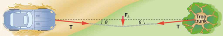
Suppose your car was mired deeply in the mud and you wanted to use the method illustrated in (Figure) to pull it out. (a) What force would you have to exert perpendicular to the center of the rope to produce a force of 12,000 N on the car if the angle is 2.00°? In this part, explicitly show how you follow the steps in the Problem-Solving Strategy for Newton’s laws of motion. (b) Real ropes stretch under such forces. What force would be exerted on the car if the angle increases to 7.00° and you still apply the force found in part (a) to its center?

What force is exerted on the tooth in (Figure) if the tension in the wire is 25.0 N? Note that the force applied to the tooth is smaller than the tension in the wire, but this is necessitated by practical considerations of how force can be applied in the mouth. Explicitly show how you follow steps in the Problem-Solving Strategy for Newton’s laws of motion.

• Use Newton’s laws since we are looking for forces.

The x -components of the tension cancel. \(\sum {F}_{x}=0\).

• This seems reasonable, since the applied tensions should be greater than the force applied to the tooth.

(Figure) shows Superhero and Trusty Sidekick hanging motionless from a rope. Superhero’s mass is 90.0 kg, while Trusty Sidekick’s is 55.0 kg, and the mass of the rope is negligible. (a) Draw a free-body diagram of the situation showing all forces acting on Superhero, Trusty Sidekick, and the rope. (b) Find the tension in the rope above Superhero. (c) Find the tension in the rope between Superhero and Trusty Sidekick. Indicate on your free-body diagram the system of interest used to solve each part.

A nurse pushes a cart by exerting a force on the handle at a downward angle \(\text{35.0º}\) below the horizontal. The loaded cart has a mass of 28.0 kg, and the force of friction is 60.0 N. (a) Draw a free-body diagram for the system of interest. (b) What force must the nurse exert to move at a constant velocity?

Construct Your Own Problem Consider the tension in an elevator cable during the time the elevator starts from rest and accelerates its load upward to some cruising velocity. Taking the elevator and its load to be the system of interest, draw a free-body diagram. Then calculate the tension in the cable. Among the things to consider are the mass of the elevator and its load, the final velocity, and the time taken to reach that velocity.

Construct Your Own Problem Consider two people pushing a toboggan with four children on it up a snow-covered slope. Construct a problem in which you calculate the acceleration of the toboggan and its load. Include a free-body diagram of the appropriate system of interest as the basis for your analysis. Show vector forces and their components and explain the choice of coordinates. Among the things to be considered are the forces exerted by those pushing, the angle of the slope, and the masses of the toboggan and children.

Unreasonable Results (a) Repeat (Figure) , but assume an acceleration of \(1\text{.}{\text{20 m/s}}^{2}\) is produced. (b) What is unreasonable about the result? (c) Which premise is unreasonable, and why is it unreasonable?

Unreasonable Results (a) What is the initial acceleration of a rocket that has a mass of \(1\text{.}\text{50}×{\text{10}}^{6}\phantom{\rule{0.25em}{0ex}}\text{kg}\) at takeoff, the engines of which produce a thrust of \(2\text{.}\text{00}×{\text{10}}^{6}\phantom{\rule{0.25em}{0ex}}\text{N}\)? Do not neglect gravity. (b) What is unreasonable about the result? (This result has been unintentionally achieved by several real rockets.) (c) Which premise is unreasonable, or which premises are inconsistent? (You may find it useful to compare this problem to the rocket problem earlier in this section.)

Intro to Physics for Non-Majors Copyright © 2012 by OSCRiceUniversity is licensed under a Creative Commons Attribution 4.0 International License , except where otherwise noted.

Share This Book

• TPC and eLearning
• What's NEW at TPC?
• Read Watch Interact
• Practice Review Test
• Teacher-Tools
• Subscription Selection
• Seat Calculator
• Ad Free Account
• Edit Profile Settings
• Classes (Version 2)
• Student Progress Edit
• Task Properties
• Export Student Progress
• Task, Activities, and Scores
• Metric Conversions Questions
• Metric System Questions
• Metric Estimation Questions
• Significant Digits Questions
• Proportional Reasoning
• Acceleration
• Distance-Displacement
• Dots and Graphs
• Graph That Motion
• Match That Graph
• Name That Motion
• Motion Diagrams
• Pos'n Time Graphs Numerical
• Pos'n Time Graphs Conceptual
• Up And Down - Questions
• Balanced vs. Unbalanced Forces
• Change of State
• Force and Motion
• Mass and Weight
• Match That Free-Body Diagram
• Net Force (and Acceleration) Ranking Tasks
• Newton's Second Law
• Normal Force Card Sort
• Recognizing Forces
• Air Resistance and Skydiving
• Solve It! with Newton's Second Law
• Which One Doesn't Belong?
• Component Addition Questions
• Head-to-Tail Vector Addition
• Projectile Mathematics
• Trajectory - Angle Launched Projectiles
• Trajectory - Horizontally Launched Projectiles
• Vector Addition
• Vector Direction
• Which One Doesn't Belong? Projectile Motion
• Forces in 2-Dimensions
• Being Impulsive About Momentum
• Explosions - Law Breakers
• Hit and Stick Collisions - Law Breakers
• Case Studies: Impulse and Force
• Impulse-Momentum Change Table
• Keeping Track of Momentum - Hit and Stick
• Keeping Track of Momentum - Hit and Bounce
• What's Up (and Down) with KE and PE?
• Energy Conservation Questions
• Energy Dissipation Questions
• Energy Ranking Tasks
• LOL Charts (a.k.a., Energy Bar Charts)
• Match That Bar Chart
• Words and Charts Questions
• Name That Energy
• Stepping Up with PE and KE Questions
• Case Studies - Circular Motion
• Circular Logic
• Forces and Free-Body Diagrams in Circular Motion
• Gravitational Field Strength
• Universal Gravitation
• Angular Position and Displacement
• Linear and Angular Velocity
• Angular Acceleration
• Rotational Inertia
• Balanced vs. Unbalanced Torques
• Getting a Handle on Torque
• Torque-ing About Rotation
• Properties of Matter
• Fluid Pressure
• Buoyant Force
• Sinking, Floating, and Hanging
• Pascal's Principle
• Flow Velocity
• Bernoulli's Principle
• Balloon Interactions
• Charge and Charging
• Charge Interactions
• Charging by Induction
• Conductors and Insulators
• Coulombs Law
• Electric Field
• Electric Field Intensity
• Polarization
• Case Studies: Electric Power
• Know Your Potential
• Light Bulb Anatomy
• I = ∆V/R Equations as a Guide to Thinking
• Parallel Circuits - ∆V = I•R Calculations
• Resistance Ranking Tasks
• Series Circuits - ∆V = I•R Calculations
• Series vs. Parallel Circuits
• Equivalent Resistance
• Period and Frequency of a Pendulum
• Pendulum Motion: Velocity and Force
• Energy of a Pendulum
• Period and Frequency of a Mass on a Spring
• Horizontal Springs: Velocity and Force
• Vertical Springs: Velocity and Force
• Energy of a Mass on a Spring
• Decibel Scale
• Frequency and Period
• Closed-End Air Columns
• Name That Harmonic: Strings
• Rocking the Boat
• Wave Basics
• Matching Pairs: Wave Characteristics
• Wave Interference
• Waves - Case Studies
• Color Addition and Subtraction
• Color Filters
• If This, Then That: Color Subtraction
• Light Intensity
• Color Pigments
• Converging Lenses
• Curved Mirror Images
• Law of Reflection
• Refraction and Lenses
• Total Internal Reflection
• Who Can See Who?
• Formulas and Atom Counting
• Atomic Models
• Bond Polarity
• Entropy Questions
• Cell Voltage Questions
• Heat of Formation Questions
• Reduction Potential Questions
• Oxidation States Questions
• Measuring the Quantity of Heat
• Hess's Law
• Oxidation-Reduction Questions
• Galvanic Cells Questions
• Thermal Stoichiometry
• Molecular Polarity
• Quantum Mechanics
• Balancing Chemical Equations
• Bronsted-Lowry Model of Acids and Bases
• Classification of Matter
• Collision Model of Reaction Rates
• Density Ranking Tasks
• Dissociation Reactions
• Complete Electron Configurations
• Elemental Measures
• Enthalpy Change Questions
• Equilibrium Concept
• Equilibrium Constant Expression
• Equilibrium Calculations - Questions
• Equilibrium ICE Table
• Intermolecular Forces Questions
• Ionic Bonding
• Lewis Electron Dot Structures
• Limiting Reactants
• Line Spectra Questions
• Mass Stoichiometry
• Measurement and Numbers
• Metals, Nonmetals, and Metalloids
• Metric Estimations
• Metric System
• Molarity Ranking Tasks
• Mole Conversions
• Name That Element
• Names to Formulas
• Names to Formulas 2
• Nuclear Decay
• Particles, Words, and Formulas
• Periodic Trends
• Precipitation Reactions and Net Ionic Equations
• Pressure Concepts
• Pressure-Temperature Gas Law
• Pressure-Volume Gas Law
• Chemical Reaction Types
• Significant Digits and Measurement
• States Of Matter Exercise
• Stoichiometry Law Breakers
• Stoichiometry - Math Relationships
• Subatomic Particles
• Spontaneity and Driving Forces
• Gibbs Free Energy
• Volume-Temperature Gas Law
• Acid-Base Properties
• Energy and Chemical Reactions
• Chemical and Physical Properties
• Valence Shell Electron Pair Repulsion Theory
• Writing Balanced Chemical Equations
• Mission CG1
• Mission CG10
• Mission CG2
• Mission CG3
• Mission CG4
• Mission CG5
• Mission CG6
• Mission CG7
• Mission CG8
• Mission CG9
• Mission EC1
• Mission EC10
• Mission EC11
• Mission EC12
• Mission EC2
• Mission EC3
• Mission EC4
• Mission EC5
• Mission EC6
• Mission EC7
• Mission EC8
• Mission EC9
• Mission RL1
• Mission RL2
• Mission RL3
• Mission RL4
• Mission RL5
• Mission RL6
• Mission KG7
• Mission RL8
• Mission KG9
• Mission RL10
• Mission RL11
• Mission RM1
• Mission RM2
• Mission RM3
• Mission RM4
• Mission RM5
• Mission RM6
• Mission RM8
• Mission RM10
• Mission LC1
• Mission RM11
• Mission LC2
• Mission LC3
• Mission LC4
• Mission LC5
• Mission LC6
• Mission LC8
• Mission SM1
• Mission SM2
• Mission SM3
• Mission SM4
• Mission SM5
• Mission SM6
• Mission SM8
• Mission SM10
• Mission KG10
• Mission SM11
• Mission KG2
• Mission KG3
• Mission KG4
• Mission KG5
• Mission KG6
• Mission KG8
• Mission KG11
• Mission F2D1
• Mission F2D2
• Mission F2D3
• Mission F2D4
• Mission F2D5
• Mission F2D6
• Mission KC1
• Mission KC2
• Mission KC3
• Mission KC4
• Mission KC5
• Mission KC6
• Mission KC7
• Mission KC8
• Mission AAA
• Mission SM9
• Mission LC7
• Mission LC9
• Mission NL1
• Mission NL2
• Mission NL3
• Mission NL4
• Mission NL5
• Mission NL6
• Mission NL7
• Mission NL8
• Mission NL9
• Mission NL10
• Mission NL11
• Mission NL12
• Mission MC1
• Mission MC10
• Mission MC2
• Mission MC3
• Mission MC4
• Mission MC5
• Mission MC6
• Mission MC7
• Mission MC8
• Mission MC9
• Mission RM7
• Mission RM9
• Mission RL7
• Mission RL9
• Mission SM7
• Mission SE1
• Mission SE10
• Mission SE11
• Mission SE12
• Mission SE2
• Mission SE3
• Mission SE4
• Mission SE5
• Mission SE6
• Mission SE7
• Mission SE8
• Mission SE9
• Mission VP1
• Mission VP10
• Mission VP2
• Mission VP3
• Mission VP4
• Mission VP5
• Mission VP6
• Mission VP7
• Mission VP8
• Mission VP9
• Mission WM1
• Mission WM2
• Mission WM3
• Mission WM4
• Mission WM5
• Mission WM6
• Mission WM7
• Mission WM8
• Mission WE1
• Mission WE10
• Mission WE2
• Mission WE3
• Mission WE4
• Mission WE5
• Mission WE6
• Mission WE7
• Mission WE8
• Mission WE9
• Vector Walk Interactive
• Name That Motion Interactive
• Kinematic Graphing 1 Concept Checker
• Kinematic Graphing 2 Concept Checker
• Graph That Motion Interactive
• Two Stage Rocket Interactive
• Rocket Sled Concept Checker
• Force Concept Checker
• Free-Body Diagrams Concept Checker
• Free-Body Diagrams The Sequel Concept Checker
• Skydiving Concept Checker
• Elevator Ride Concept Checker
• Vector Addition Concept Checker
• Vector Walk in Two Dimensions Interactive
• Name That Vector Interactive
• River Boat Simulator Concept Checker
• Projectile Simulator 2 Concept Checker
• Projectile Simulator 3 Concept Checker
• Hit the Target Interactive
• Turd the Target 1 Interactive
• Turd the Target 2 Interactive
• Balance It Interactive
• Go For The Gold Interactive
• Egg Drop Concept Checker
• Fish Catch Concept Checker
• Exploding Carts Concept Checker
• Collision Carts - Inelastic Collisions Concept Checker
• Its All Uphill Concept Checker
• Stopping Distance Concept Checker
• Chart That Motion Interactive
• Roller Coaster Model Concept Checker
• Uniform Circular Motion Concept Checker
• Horizontal Circle Simulation Concept Checker
• Vertical Circle Simulation Concept Checker
• Race Track Concept Checker
• Gravitational Fields Concept Checker
• Orbital Motion Concept Checker
• Angular Acceleration Concept Checker
• Balance Beam Concept Checker
• Torque Balancer Concept Checker
• Aluminum Can Polarization Concept Checker
• Charging Concept Checker
• Name That Charge Simulation
• Coulomb's Law Concept Checker
• Electric Field Lines Concept Checker
• Put the Charge in the Goal Concept Checker
• Circuit Builder Concept Checker (Series Circuits)
• Circuit Builder Concept Checker (Parallel Circuits)
• Circuit Builder Concept Checker (∆V-I-R)
• Circuit Builder Concept Checker (Voltage Drop)
• Equivalent Resistance Interactive
• Pendulum Motion Simulation Concept Checker
• Mass on a Spring Simulation Concept Checker
• Particle Wave Simulation Concept Checker
• Boundary Behavior Simulation Concept Checker
• Slinky Wave Simulator Concept Checker
• Simple Wave Simulator Concept Checker
• Wave Addition Simulation Concept Checker
• Standing Wave Maker Simulation Concept Checker
• Color Addition Concept Checker
• Painting With CMY Concept Checker
• Stage Lighting Concept Checker
• Filtering Away Concept Checker
• InterferencePatterns Concept Checker
• Young's Experiment Interactive
• Plane Mirror Images Interactive
• Who Can See Who Concept Checker
• Optics Bench (Mirrors) Concept Checker
• Name That Image (Mirrors) Interactive
• Refraction Concept Checker
• Total Internal Reflection Concept Checker
• Optics Bench (Lenses) Concept Checker
• Kinematics Preview
• Velocity Time Graphs Preview
• Moving Cart on an Inclined Plane Preview
• Stopping Distance Preview
• Cart, Bricks, and Bands Preview
• Fan Cart Study Preview
• Friction Preview
• Coffee Filter Lab Preview
• Friction, Speed, and Stopping Distance Preview
• Up and Down Preview
• Projectile Range Preview
• Ballistics Preview
• Juggling Preview
• Marshmallow Launcher Preview
• Air Bag Safety Preview
• Colliding Carts Preview
• Collisions Preview
• Engineering Safer Helmets Preview
• Push the Plow Preview
• Its All Uphill Preview
• Energy on an Incline Preview
• Modeling Roller Coasters Preview
• Hot Wheels Stopping Distance Preview
• Ball Bat Collision Preview
• Energy in Fields Preview
• Weightlessness Training Preview
• Roller Coaster Loops Preview
• Universal Gravitation Preview
• Keplers Laws Preview
• Kepler's Third Law Preview
• Charge Interactions Preview
• Sticky Tape Experiments Preview
• Wire Gauge Preview
• Voltage, Current, and Resistance Preview
• Light Bulb Resistance Preview
• Series and Parallel Circuits Preview
• Thermal Equilibrium Preview
• Linear Expansion Preview
• Heating Curves Preview
• Electricity and Magnetism - Part 1 Preview
• Electricity and Magnetism - Part 2 Preview
• Vibrating Mass on a Spring Preview
• Period of a Pendulum Preview
• Wave Speed Preview
• Slinky-Experiments Preview
• Standing Waves in a Rope Preview
• Sound as a Pressure Wave Preview
• DeciBel Scale Preview
• DeciBels, Phons, and Sones Preview
• Sound of Music Preview
• Shedding Light on Light Bulbs Preview
• Models of Light Preview
• Electromagnetic Radiation Preview
• Electromagnetic Spectrum Preview
• EM Wave Communication Preview
• Digitized Data Preview
• Light Intensity Preview
• Concave Mirrors Preview
• Object Image Relations Preview
• Snells Law Preview
• Reflection vs. Transmission Preview
• Magnification Lab Preview
• Reactivity Preview
• Ions and the Periodic Table Preview
• Periodic Trends Preview
• Intermolecular Forces Preview
• Melting Points and Boiling Points Preview
• Reaction Rates Preview
• Ammonia Factory Preview
• Stoichiometry Preview
• Nuclear Chemistry Preview
• Gaining Teacher Access
• Tasks and Classes
• Tasks - Classic
• Subscription
• Subscription Locator
• 1-D Kinematics
• Newton's Laws
• Vectors - Motion and Forces in Two Dimensions
• Momentum and Its Conservation
• Work and Energy
• Circular Motion and Satellite Motion
• Thermal Physics
• Static Electricity
• Electric Circuits
• Vibrations and Waves
• Sound Waves and Music
• Light and Color
• Reflection and Mirrors
• About the Physics Interactives
• Task Tracker
• Usage Policy
• Newtons Laws
• Vectors and Projectiles
• Forces in 2D
• Momentum and Collisions
• Circular and Satellite Motion
• Balance and Rotation
• Electromagnetism
• Waves and Sound
• Atomic Physics
• Forces in Two Dimensions
• Work, Energy, and Power
• Circular Motion and Gravitation
• Sound Waves
• 1-Dimensional Kinematics
• Circular, Satellite, and Rotational Motion
• Einstein's Theory of Special Relativity
• Waves, Sound and Light
• QuickTime Movies
• About the Concept Builders
• Pricing For Schools
• Directions for Version 2
• Measurement and Units
• Relationships and Graphs
• Rotation and Balance
• Vibrational Motion
• Reflection and Refraction
• Teacher Accounts
• Task Tracker Directions
• Kinematic Concepts
• Kinematic Graphing
• Wave Motion
• Sound and Music
• About CalcPad
• 1D Kinematics
• Vectors and Forces in 2D
• Simple Harmonic Motion
• Rotational Kinematics
• Rotation and Torque
• Rotational Dynamics
• Electric Fields, Potential, and Capacitance
• Transient RC Circuits
• Light Waves
• Units and Measurement
• Stoichiometry
• Molarity and Solutions
• Thermal Chemistry
• Acids and Bases
• Kinetics and Equilibrium
• Solution Equilibria
• Oxidation-Reduction
• Nuclear Chemistry
• Newton's Laws of Motion
• Work and Energy Packet
• Static Electricity Review
• NGSS Alignments
• 1D-Kinematics
• Projectiles
• Circular Motion
• Magnetism and Electromagnetism
• Graphing Practice
• About the ACT
• ACT Preparation
• For Teachers
• Other Resources
• Solutions Guide
• Solutions Guide Digital Download
• Motion in One Dimension
• Work, Energy and Power
• TaskTracker
• Other Tools
• Algebra Based Physics
• Frequently Asked Questions
• Purchasing the Download
• Purchasing the CD
• Purchasing the Digital Download
• About the NGSS Corner
• NGSS Search
• Force and Motion DCIs - High School
• Energy DCIs - High School
• Wave Applications DCIs - High School
• Force and Motion PEs - High School
• Energy PEs - High School
• Wave Applications PEs - High School
• Crosscutting Concepts
• The Practices
• Physics Topics
• NGSS Corner: Activity List
• NGSS Corner: Infographics
• About the Toolkits
• Position-Velocity-Acceleration
• Position-Time Graphs
• Velocity-Time Graphs
• Newton's First Law
• Newton's Second Law
• Newton's Third Law
• Terminal Velocity
• Projectile Motion
• Forces in 2 Dimensions
• Impulse and Momentum Change
• Momentum Conservation
• Work-Energy Fundamentals
• Work-Energy Relationship
• Roller Coaster Physics
• Satellite Motion
• Electric Fields
• Circuit Concepts
• Series Circuits
• Parallel Circuits
• Describing-Waves
• Wave Behavior Toolkit
• Standing Wave Patterns
• Resonating Air Columns
• Wave Model of Light
• Plane Mirrors
• Curved Mirrors
• Teacher Guide
• Using Lab Notebooks
• Current Electricity
• Light Waves and Color
• Reflection and Ray Model of Light
• Refraction and Ray Model of Light
• Classes (Legacy Version)
• Teacher Resources
• Subscriptions

• Newton's Laws
• Einstein's Theory of Special Relativity
• About Concept Checkers
• School Pricing
• Newton's Laws of Motion
• Newton's First Law
• Newton's Third Law

Work-Energy Practice Problems Video Tutorial

The Work-Energy Practice Problems Video Tutorial focuses on the use of work-energy concepts to solve problems. After providing a background and a short strategy, Mr. H steps through detailed solutions to six example problems involving work and energy. Learn how to use the concepts to solve for speed, height, and distance.  The video lesson answers the following question:

• How do you use the work-energy relationship to solve problems involving speed, height, and distance?

View Video Tutorial

Help us help you.

Physics Problems with Solutions

• Electric Circuits
• Electrostatic
• Calculators
• Practice Tests
• Simulations

• Uniform Acceleration Motion: Problems with Solutions

Problems on velocity and uniform acceleration are presented along with detailed solutions and tutorials can also be found in this website.

From rest, a car accelerated at 8 m/s 2 for 10 seconds. a) What is the position of the car at the end of the 10 seconds? b) What is the velocity of the car at the end of the 10 seconds? Solution to Problem 1

With an initial velocity of 20 km/h, a car accelerated at 8 m/s 2 for 10 seconds. a) What is the position of the car at the end of the 10 seconds? b) What is the velocity of the car at the end of the 10 seconds? Solution to Problem 2

A car accelerates uniformly from 0 to 72 km/h in 11.5 seconds. a) What is the acceleration of the car in m/s 2 ? b) What is the position of the car by the time it reaches the velocity of 72 km/h? Solution to Problem 3

An object is thrown straight down from the top of a building at a speed of 20 m/s. It hits the ground with a speed of 40 m/s. a) How high is the building? b) How long was the object in the air? Solution to Problem 4

A train brakes from 40 m/s to a stop over a distance of 100 m. a) What is the acceleration of the train? b) How much time does it take the train to stop? Solution to Problem 5

A boy on a bicycle increases his velocity from 5 m/s to 20 m/s in 10 seconds. a) What is the acceleration of the bicycle? b) What distance was covered by the bicycle during the 10 seconds? Solution to Problem 6

a) How long does it take an airplane to take off if it needs to reach a speed on the ground of 350 km/h over a distance of 600 meters (assume the plane starts from rest)? b) What is the acceleration of the airplane over the 600 meters? Solution to Problem 7

Starting from a distance of 20 meters to the left of the origin and at a velocity of 10 m/s, an object accelerates to the right of the origin for 5 seconds at 4 m/s 2 . What is the position of the object at the end of the 5 seconds of acceleration? Solution to Problem 8

What is the smallest distance, in meters, needed for an airplane touching the runway with a velocity of 360 km/h and an acceleration of -10 m/s 2 to come to rest? Solution to Problem 9

Problem 10:

To approximate the height of a water well, Martha and John drop a heavy rock into the well. 8 seconds after the rock is dropped, they hear a splash caused by the impact of the rock on the water. What is the height of the well. (Speed of sound in air is 340 m/s). Solution to Problem 10

Problem 11:

A rock is thrown straight up and reaches a height of 10 m. a) How long was the rock in the air? b) What is the initial velocity of the rock? Solution to Problem 11

Problem 12:

A car accelerates from rest at 1.0 m/s 2 for 20.0 seconds along a straight road . It then moves at a constant speed for half an hour. It then decelerates uniformly to a stop in 30.0 s. Find the total distance covered by the car. Solution to Problem 12

More References and links

• Velocity and Speed: Tutorials with Examples
• Velocity and Speed: Problems with Solutions
• Acceleration: Tutorials with Examples
• Uniform Acceleration Motion: Equations with Explanations

Popular Pages

• Privacy Policy

• Exam Center
• Ticket Center
• Flash Cards

Magnetic Field: Solved Problems for grade 12 and AP Physics

On this page, some Problems on magnetic fields for high school and colleges are solved. Each section is separated for easier reading. 

Magnetic Field Problems: Force on a single Moving Charge

Problem (1): A proton moves with a speed of $2\times 10^6 \,\rm m/s$ at an angle of $30^\circ$ with the direction of a magnetic field of $0.2\,\rm T$ in the negative $y$-direction.  (a) What is the magnitude and direction of the magnetic force on the proton? (b) What acceleration does undergo by the proton?

Solution : The magnitude of the magnetic force on a single charge moving at speed of $v$ in a uniform magnetic field of $B$ is determined by the formula $F=qvB\sin \theta$ where $\theta$ is the angle between velocity and magnetic field. $q$ is also the magnitude of the charge, which in this case is $q=1.6\times 10^{-19}\,\rm C$. (a) Substituting all numerical values into the above equation, we have \begin{align*} F&=qvB\sin\theta \\\\ &=(1.6\times 10^{-19})(2\times 10^6)(0.3) \sin 30^\circ \\\\ &=4.8\times 10^{-14}\,\rm N \end{align*}  An extremely small force. This was the magnitude of the magnetic force. To find the direction of the magnetic force on a positive moving charge , we should use the right-hand rule. 

First, identify the directions of $\vec{B}$ and $\vec{v}$ as illustrated in the figure below. Now, according to this rule, put your right fingers along the direction of the charge's velocity $\vec{v}$, then curl your fingers toward the magnetic field $\vec{B}$ through the smaller angle. As a result, your thumb will point in the direction of the magnetic force $\vec{F}$ exerted on the positive charge.

In this case, the thumb points out of the page $\odot$. 

(b) Applying Newton's second law, $F=ma$ and solving for $a$ gives \[a=\frac{F}{m}=\frac{4.8\times 10^{-14}}{1.67\times 10^{-27}}=2.87\times 10^{13}\,\rm \frac{m}{s^2}\] Although the magnetic force exerted on the proton was quite small, it experiences a huge acceleration since its mass is also extremely small.

Problem (2): An electron experiences a force of $3.5\times 10^{-15}\,\rm N$ when moving at an angle of $37^\circ$ with the direction of a magnetic field of $2.5\times 10^{-3}\,\rm T$. How fast was the electron?

Solution : Again, the magnitude of the magnetic force exerted by a uniform magnetic field $B$ on a charged particle moving at $v$ with an angle of $\theta$ relative to the $\vec{B}$ is found to be $F=qvB\sin\theta$. Substituting the numerical values into it and solving for $v$, gives \begin{align*} v&=\frac{F}{qB\sin\theta} \\\\ &=\frac{3.5\times 10^{-15}}{(1.6\times 10^{-19})(2.5\times 10^{-3})\sin 37^\circ} \\\\ &=13.7\times 10^6\quad\rm m/s \end{align*} Note that in this formula, only the magnitude of the electric charge is included not its sign. The sign of charge determines the direction of the magnetic force on it. 

Problem (3): In the following diagrams, find the direction of the magnetic force on a negative charge. ($\otimes$ and $\odot$ indicate the directions into and out of the page, respectively.)

Solution : Notice that in this magnetic field Problem, the charge is negative, so the right-hand rule must be applied with caution. According to this rule, put outstretched fingers of your right hand along the direction of the velocity $\vec{v}$ and curl them toward the magnetic field vector $\vec{B}$ through the smaller angle between them. In this case, your thumb points in the direction of the force. 

This instruction is only for positive charges. If the charge was negative, simply reverse the direction of the force. 

By doing so, the correct force direction on each diagram is shown below. The blue dotted arrows show the force direction if the charge had been positive. 

In the right lower diagram the angle between $\vec{B}$ and $\vec{v}$ is $\theta=180^\circ$, so $\sin \theta=0$, and no force is applied to the particle, $F=0$.

Solution : Place your right-hand fingers in the direction of the velocity $v$ and curl them toward the direction of the magnetic field $B$. The direction of the thumb is in the direction of the force. Note that $\otimes$ and $\odot$ represent vectors pointing into the page and out of the page, respectively. 

In the left lower diagram the angle $\theta=180^\circ$, so $\sin 180^\circ=0$, and the force is zero. Pay attention to the sign of the electric charge. For a negative charge, the force direction obtained by the right-hand rule must be reversed.

Solution : (a) Substituting all known values into the following formula and solve for $F$.\begin{align*} F&=qvB\sin\theta \\ &=(1.6\times 10^{-19})(7.5\times 10^6)(45) \sin 45^\circ \\ &=3.8\times 10^{-11}\,\rm N \end{align*}  (b) The right-hand rule gives us the direction of the magnetic force into the plane of the page, $\otimes$. Place the fingers of your right hand along the velocity vector (red arrow) and rotate them toward the magnetic field. As a result, your thumb, which shows the direction of the force, points into the page, $\otimes$.

Problem (6): An alpha particle moving at a speed of $2\times 10^7 \,\rm m/s$ toward the positive $z$-direction perpendicularly enters a uniform magnetic field $\vec{B}$ and experiences an acceleration of $1.0\times 10^{13}\,\rm m/s^2$ in the positive $x$-direction. Find the magnitude and direction of the magnetic field? 

Solution : The mass of an alpha particle is four times $m_{\alpha}=4m_p$ and its charge is twice $q_{\alpha}=2e$ that of a proton.

The alpha particle's velocity is given as $\vec{v}=2\times 10^7\, (+\hat{k})\quad \rm m/s$. 

In this magnetic field Problem, the magnitude and direction of the acceleration acquired by the alpha particle was given. We can use these information to find the magnitude and direction of the applied force to it as below \begin{align*} F&=m_{\alpha}a \\\\ &=(4)(1.67\times 10^{-27})(1.0\times 10^{13}) \\\\ &=6.68\times 10^{-14}\quad \rm N \end{align*} This force directed toward the positive $x$-direction, i.e., $+\hat{i}$, in the same direction of the acceleration.

As you can see, in the following diagram the angle between $\vec{v}$ and $\vec{B}$ is $90^\circ$, so $\sin \theta=1$. 

After collecting all these the given information, use the magnetic force formula, $F=qvB\sin\theta$, and solve for $B$ to find the unknown magnitude of the magnetic field \begin{align*} B&=\frac{F}{qv\sin\theta}\\\\ &=\frac{6.68\times 10^{-14}}{(2)(1.6\times 10^{-19}) (2\times 10^7)} \\\\ &=0.01\quad \rm T\end{align*} Now, apply the right-hand rule for a positive charge to find the direction of $\vec{B}$. Here, we choose a coordinate system in which out of the page indicates the positive $z$-direction. 

Hold your right hand so that the four fingers point in the $\vec{v}$ (out of the page) and the thumb points toward the $\vec{F}$ (to the right). In this situation, your palm faces in the direction of the magnetic field (up the page). 

  Problem (7): An electron with a kinetic energy of $1.5\,\rm keV$ perpendicularly enters a $0.02-\rm T$ magnetic field. Determine the radius of its path as it moves through this uniform field? 

Solution : First note that $\rm keV$ is a unit of energy in the subatomic level that converts into the usual units of energy, the joules, as below \begin{align*} \rm 1\,keV &=1\times 10^3 \times (1.6\times 10^{-19}) \,J \\ &=1.6\times 10^{-16}\,J\end{align*} By knowing the kinetic energy $K=\frac 12 mv^2$, we can find the particle's velocity as below \begin{align*} v&=\sqrt{\frac{2K}{m}} \\\\ &=\sqrt{\frac{2(1.5)(1.6\times 10^{-16})}{9.11\times 10^{-31}}} \\\\&=2.3\times 10^7\,\rm m/s \end{align*} When a charged particle enters a region of uniform magnetic field at right angle with a speed of $v$, the magnetic field forces it to move in a circular path of radius $r$. This force, whose magnitude is found by $qvB\sin\theta$, serves as a centripetal force radially toward the center of the circle. As we learned in the circular motion Problems section, the acceleration that the object acquire is $a_c=\frac{mv^2}{r}$. Consequently, we have \begin{gather*} F=ma_c \\\\ qvB\sin 90^\circ=\frac{mv^2}{r} \\\\ \Rightarrow \quad r=\frac{mv}{qB} \end{gather*} It is better to memorize this important formula. It always gives the radius of a charged particle moving through a uniform $\vec{B}$ perpendicularly. 

Hence, the value of radius is obtained as follows \begin{align*} r&=\frac{(9.11\times 10^{-31})(2.3\times 10^7)}{(1.6\times 10^{-19})(0.02)} \\\\ &=0.65\times 10^{-2}\,\rm m\end{align*} Therefore, this electron having such energy when enters a $0.02\,\rm T$ field bends around a circle of radius $0.65\,\rm mm$.  For more information about this bending, refer to the helical motion in a magnetic field .

Problem (8): An electron undergoes the greatest force of magnitude $3.2\times 10^{-13}\,\rm N$, vertically upward, when it travels northward at a speed of $5\times 10^6 \,\rm m/s$ in a uniform magnetic field of unknown strength. What is the magnitude and direction of the magnetic field? 

Solution : in all magnetic field questions, the greatest force occurs when the angle between $\vec{v}$ and $\vec{B}$ is $90^\circ$. In this case, $\sin\theta=1$. By solving the equation $F=qvB\sin\theta$ for $B$ and substituting the numbers into it, we get \begin{align*} B&=\frac{F}{qv} \\\\ &=\frac{3.2\times 10^{-13}}{(1.6\times 10^{-19})(5\times 10^6)} \\\\ &=0.4\,\rm T \end{align*} To find the direction of the field, first of all, set a coordinate system and specify all the directions on it as below. In this standard coordinate system, used when geographical direction included in the Problem, we assume north and south directions as into $\otimes$ and out of the page $\odot$, respectively.

Place the four fingers of your right hand in the direction of velocity $\vec{v}$ so that your thumb points to the force direction. In this case, your palm faces toward the magnetic field. This is the right-hand rule for a positive charge. 

Doing so, your palm will be toward the left (or west) but the electric charge of the electron is negative so you must reverse that direction (which is shown as a red dotted arrow) to find the correct direction of the field.

Problem (9): A proton traveling with a speed of $2.4\times 10^6\,\rm m/s$ through a uniform magnetic field of strength $2.5\,\rm T$ experiences a force of magnitude $4.8\times 10^{-13}\,\rm N$. At what angle does the electron enter the field? 

Solution : here, the unknown is the angle between $\vec{v}$ and $\vec{B}$. Applying the magnetic force formula, $F=qvB\sin\theta$, and solving for the unknown angle $\theta$ gives \begin{align*} \sin\theta &=\frac{F}{qvB} \\\\ &=\frac{4.8\times 10^{-13}}{(1.6\times 10^{-19})(2.4\times 10^6)(2.5)} \\\\&= 0.5 \end{align*} Taking the inverse sine of both sides, gives us the desired angle \[\theta=30^\circ\] 

Problem (10): The path of a negatively charged particle traveling through a magnetic field is shown in the figure below. What is the direction of the $\vec{B}$ field? 

Solution : 

Magnetic Field Problems: Force on Electric Current

Problem (11): In each of the following diagrams, a current-carrying wire is shown into a uniform external magnetic field. Find the direction of the magnetic force for each diagram.

Solution : Place outstretched fingers of your right hand along the direction of the current. For the left diagram, your fingers must point down the page. Now, curl them toward the magnetic field $B$ which is out of the plane of the page. As a result, your thumbs, which represent the force, points to the left. 

For the right diagram, there is an interesting point. If look closely, the current is out of the page and the field is into the page, so the angle between them is $180^\circ$ and we know that $\sin 180^\circ=0$. Consequently, there is no force acting on this wire. 

Problem (12): Find the magnitude of the force per meter exerted on a straight wire carrying a current of $3.5\,\rm A$ through a magnetic field of $0.85\,\rm T$ when  (a) it is placed perpendicular to the $\vec{B}$. (b) it makes an angle of $37^\circ$ with the field. 

Solution : When a straight wire of length $\ell$ carrying a current $i$ passes through a uniform external magnetic field $\vec{B}$, it experiences a force of magnitude $F=i\ell B\sin \theta$ where $\theta$ is the angle between the direction of the current and $\vec{B}$. 

The force ''per meter'' means the force acted on one meter of the wire, so $\ell=1\,\rm m$. 

(a) In this case, we have $\theta=90^\circ$, so $\sin\theta=1$. Thus, the magnitude of the force is found to be \begin{align*} F&=i\ell B\sin\theta \\&=(3.5)(1)(0.85) \\&=2.975\quad \rm N \end{align*} (b) Similarly, we have \begin{align*} F&=i\ell B\sin\theta \\&=(3.5)(1)(0.85) \sin 37^\circ \\&=1.785\quad \rm N \end{align*} 

Problem (13): A straight wire carrying a current of $4\,\rm A$ is placed perpendicularly in a uniform magnetic field of strength $0.45\,\rm T$. What is the magnitude of the magnetic force on a $35-\rm cm$-long section of this wire? 

Solution : All the required information to substitute into the magnetic force formula is given. Hence, we have \begin{align*} F&=i\ell B\sin\theta \\&=(4)(0.35)(0.45) \sin 90^\circ \\&=0.63\quad \rm N \end{align*} 

Problem (14): An straight section of a wire $0.40\,\rm m$ long carrying a steady current of $2.5\,\rm A$ toward the $+x$ direction lies in a region where a uniform magnetic field of strength $B=1.5\,\rm T$ to the $+z$ direction is present. What is the magnitude and direction of the magnetic force on this section of wire?

Solution : In this magnetic field Problem, the angle between $\vec{B}$ and the direction of the electric current is $90^\circ$, so $\sin\theta=1$. The magnitude of the magnetic force is also determined as below \begin{align*} F&=i\ell B\sin \theta \\ &=(2.5)(0.40)(1.5) \\ &=1.5\quad \rm N\end{align*} To find the direction of the force acting on the wire, do the following:  Point the fingers of your right hand in the direction of the current $i$ and curl them toward the magnetic field direction. Your thumb, then, points in the direction of the magnetic force. This is the right-hand rule for finding the magnetic force on a current-carrying wire in a uniform $\vec{B}$. 

Problem (15): At a location where the Earth's magnetic field is $0.5\,\rm G$ from south to north, there is a straight wire of length $2\,\rm m$ that carries a current of $1.5\,\rm A$. In each of the following situations, find the magnitude and direction of the magnetic force exerted on the wire due to the earth's magnetic field?  (a) a current flowing from west to east. (b) a current flowing vertically upward. (c) a current flowing north to south. 

Solution : The magnitude of the magnetic force is obtained by the equation $F=i\ell B\sin\theta$ and its direction is also found by the right-hand rule. To solve such magnetic field Problems, first set up a coordinate system and specify each direction on it as below. In this coordinate system south and north directions are shown by the symbols $\odot$ and $\otimes$ means out of and into the page, respectively.

The Earth's magnetic field is from south to north, which we can imagine as an arrow points into the page, i.e., $\otimes$. The gauss, $\rm G$ is another unit for magnetic field and is related to the tesla by $\rm 1\, G=10^{-4} \, T$.

  Problem (16): In a region of space, a magnetic force per unit length of $0.24\,\rm N/m$ toward the positive $z$-axis exerts on a current of $I=10\,\rm A$ directed along the positive $y$-direction and perpendicular to the magnetic field $\vec{B}$. Determine the magnitude and direction of the magnetic field?

Solution : the magnitude of the magnetic force on a wire of length $\ell$ carrying current $i$ in a uniform external magnetic field $\vec{B}$, is determined by the following formula \[F=i\ell B\sin\theta\] where $\theta$ is the angle between the direction of the current and the direction of the magnetic field. When this angle is $90^\circ$, the magnetic force acted on the wire is maximum.

Here, the maximum ($\theta=90^\circ$) force per unit length was given $F/\ell=0.24\,\rm N/m$. Substituting the given data into the above formula and solving for $B$ gives \begin{align*} B&=\frac{F}{i\ell} \\\\ &=\frac{0.24}{10}\\\\ &=0.024\quad \rm T \end{align*} The right-hand rule gives us the direction of $\vec{B}$. 

To find the magnetic force direction on a wire carrying current in a uniform magnetic field, the following version of the right-hand rule must be applied. 

We were asked to make a situation in which the tension in the wires be zero. This holds when the downward conductor's weight force $mg$ is balanced with an upward magnetic force $i\ell B$. Note that, here, the angle between $\vec{B}$ and the wire is $\theta=90^\circ$, so $\sin \theta=1$.

Magnetic Field Due to a Long Straight Wire

Problem (18): A current of $20\,\rm A$ flows vertically upward in a straight wire. What is the magnitude and direction of the magnetic field due to this long wire at a location $15\,\rm cm$ away and on the left side of the wire?

Solution : The magnitude of the magnetic field due to a long straight wire near to it is found as follows \[B=\frac{\mu_0 I}{2\pi r} \] where $\mu_0=4\pi\times 10^{-7}\,\rm T\cdot m/A$ is called the permeability of free space. Plug in the known values gives \begin{align*} B&=\frac{(4\pi\times 10^{-7})(20)}{2\pi\times 0.15} \\\\ &=2\times 10^{-5}\,\rm T\end{align*} To find the direction of the magnetic field due this long wire, we must use the following version of the right-hand rule: 

Grasp the wire in your right hand so that the thumb points in the direction of the current. Now, wrap your four fingers around the wire. This is the direction of the $\vec{B}$. 

Doing so, in this case, at the point $P$ on the left side of the wire the fingers will come out of the paper, $\otimes$. 

Similarly, on the right side, the four fingers will come into the paper, $\otimes$. These are the directions of the $\vec{B}$ at those points.   

Author : Dr. Ali Nemati Published : 3/2/2022

© 2015 All rights reserved. by Physexams.com

• school Campus Bookshelves
• menu_book Bookshelves
• perm_media Learning Objects
• login Login
• how_to_reg Request Instructor Account
• hub Instructor Commons
• Download Page (PDF)
• Download Full Book (PDF)
• Periodic Table
• Physics Constants
• Scientific Calculator
• Reference & Cite
• Tools expand_more
• Readability

selected template will load here

This action is not available.

1.8: Solving Problems in Physics

• Last updated
• Save as PDF
• Page ID 46031

\( \newcommand{\vecs}[1]{\overset { \scriptstyle \rightharpoonup} {\mathbf{#1}} } \)

\( \newcommand{\vecd}[1]{\overset{-\!-\!\rightharpoonup}{\vphantom{a}\smash {#1}}} \)

\( \newcommand{\id}{\mathrm{id}}\) \( \newcommand{\Span}{\mathrm{span}}\)

( \newcommand{\kernel}{\mathrm{null}\,}\) \( \newcommand{\range}{\mathrm{range}\,}\)

\( \newcommand{\RealPart}{\mathrm{Re}}\) \( \newcommand{\ImaginaryPart}{\mathrm{Im}}\)

\( \newcommand{\Argument}{\mathrm{Arg}}\) \( \newcommand{\norm}[1]{\| #1 \|}\)

\( \newcommand{\inner}[2]{\langle #1, #2 \rangle}\)

\( \newcommand{\Span}{\mathrm{span}}\)

\( \newcommand{\id}{\mathrm{id}}\)

\( \newcommand{\kernel}{\mathrm{null}\,}\)

\( \newcommand{\range}{\mathrm{range}\,}\)

\( \newcommand{\RealPart}{\mathrm{Re}}\)

\( \newcommand{\ImaginaryPart}{\mathrm{Im}}\)

\( \newcommand{\Argument}{\mathrm{Arg}}\)

\( \newcommand{\norm}[1]{\| #1 \|}\)

\( \newcommand{\Span}{\mathrm{span}}\) \( \newcommand{\AA}{\unicode[.8,0]{x212B}}\)

\( \newcommand{\vectorA}[1]{\vec{#1}}      % arrow\)

\( \newcommand{\vectorAt}[1]{\vec{\text{#1}}}      % arrow\)

\( \newcommand{\vectorB}[1]{\overset { \scriptstyle \rightharpoonup} {\mathbf{#1}} } \)

\( \newcommand{\vectorC}[1]{\textbf{#1}} \)

\( \newcommand{\vectorD}[1]{\overrightarrow{#1}} \)

\( \newcommand{\vectorDt}[1]{\overrightarrow{\text{#1}}} \)

\( \newcommand{\vectE}[1]{\overset{-\!-\!\rightharpoonup}{\vphantom{a}\smash{\mathbf {#1}}}} \)

Learning Objectives

• Describe the process for developing a problem-solving strategy.
• Explain how to find the numerical solution to a problem.
• Summarize the process for assessing the significance of the numerical solution to a problem.

Problem-solving skills are clearly essential to success in a quantitative course in physics. More important, the ability to apply broad physical principles—usually represented by equations—to specific situations is a very powerful form of knowledge. It is much more powerful than memorizing a list of facts. Analytical skills and problem-solving abilities can be applied to new situations whereas a list of facts cannot be made long enough to contain every possible circumstance. Such analytical skills are useful both for solving problems in this text and for applying physics in everyday life.

As you are probably well aware, a certain amount of creativity and insight is required to solve problems. No rigid procedure works every time. Creativity and insight grow with experience. With practice, the basics of problem solving become almost automatic. One way to get practice is to work out the text’s examples for yourself as you read. Another is to work as many end-of-section problems as possible, starting with the easiest to build confidence and then progressing to the more difficult. After you become involved in physics, you will see it all around you, and you can begin to apply it to situations you encounter outside the classroom, just as is done in many of the applications in this text.

Although there is no simple step-by-step method that works for every problem, the following three-stage process facilitates problem solving and makes it more meaningful. The three stages are strategy, solution, and significance. This process is used in examples throughout the book. Here, we look at each stage of the process in turn.

Strategy is the beginning stage of solving a problem. The idea is to figure out exactly what the problem is and then develop a strategy for solving it. Some general advice for this stage is as follows:

• Examine the situation to determine which physical principles are involved . It often helps to draw a simple sketch at the outset. You often need to decide which direction is positive and note that on your sketch. When you have identified the physical principles, it is much easier to find and apply the equations representing those principles. Although finding the correct equation is essential, keep in mind that equations represent physical principles, laws of nature, and relationships among physical quantities. Without a conceptual understanding of a problem, a numerical solution is meaningless.
• Make a list of what is given or can be inferred from the problem as stated (identify the “knowns”) . Many problems are stated very succinctly and require some inspection to determine what is known. Drawing a sketch be very useful at this point as well. Formally identifying the knowns is of particular importance in applying physics to real-world situations. For example, the word stopped means the velocity is zero at that instant. Also, we can often take initial time and position as zero by the appropriate choice of coordinate system.
• Identify exactly what needs to be determined in the problem (identify the unknowns). In complex problems, especially, it is not always obvious what needs to be found or in what sequence. Making a list can help identify the unknowns.
• Determine which physical principles can help you solve the problem . Since physical principles tend to be expressed in the form of mathematical equations, a list of knowns and unknowns can help here. It is easiest if you can find equations that contain only one unknown—that is, all the other variables are known—so you can solve for the unknown easily. If the equation contains more than one unknown, then additional equations are needed to solve the problem. In some problems, several unknowns must be determined to get at the one needed most. In such problems it is especially important to keep physical principles in mind to avoid going astray in a sea of equations. You may have to use two (or more) different equations to get the final answer.

The solution stage is when you do the math. Substitute the knowns (along with their units) into the appropriate equation and obtain numerical solutions complete with units . That is, do the algebra, calculus, geometry, or arithmetic necessary to find the unknown from the knowns, being sure to carry the units through the calculations. This step is clearly important because it produces the numerical answer, along with its units. Notice, however, that this stage is only one-third of the overall problem-solving process.

Significance

After having done the math in the solution stage of problem solving, it is tempting to think you are done. But, always remember that physics is not math. Rather, in doing physics, we use mathematics as a tool to help us understand nature. So, after you obtain a numerical answer, you should always assess its significance:

• Check your units . If the units of the answer are incorrect, then an error has been made and you should go back over your previous steps to find it. One way to find the mistake is to check all the equations you derived for dimensional consistency. However, be warned that correct units do not guarantee the numerical part of the answer is also correct.
• Check the answer to see whether it is reasonable. Does it make sense? This step is extremely important: –the goal of physics is to describe nature accurately. To determine whether the answer is reasonable, check both its magnitude and its sign, in addition to its units. The magnitude should be consistent with a rough estimate of what it should be. It should also compare reasonably with magnitudes of other quantities of the same type. The sign usually tells you about direction and should be consistent with your prior expectations. Your judgment will improve as you solve more physics problems, and it will become possible for you to make finer judgments regarding whether nature is described adequately by the answer to a problem. This step brings the problem back to its conceptual meaning. If you can judge whether the answer is reasonable, you have a deeper understanding of physics than just being able to solve a problem mechanically.
• Check to see whether the answer tells you something interesting. What does it mean? This is the flip side of the question: Does it make sense? Ultimately, physics is about understanding nature, and we solve physics problems to learn a little something about how nature operates. Therefore, assuming the answer does make sense, you should always take a moment to see if it tells you something about the world that you find interesting. Even if the answer to this particular problem is not very interesting to you, what about the method you used to solve it? Could the method be adapted to answer a question that you do find interesting? In many ways, it is in answering questions such as these science that progresses.

Help | Advanced Search

Physics > Fluid Dynamics

Title: an analysis and solution of ill-conditioning in physics-informed neural networks.

Abstract: Physics-informed neural networks (PINNs) have recently emerged as a novel and popular approach for solving forward and inverse problems involving partial differential equations (PDEs). However, achieving stable training and obtaining correct results remain a challenge in many cases, often attributed to the ill-conditioning of PINNs. Nonetheless, further analysis is still lacking, severely limiting the progress and applications of PINNs in complex engineering problems. Drawing inspiration from the ill-conditioning analysis in traditional numerical methods, we establish a connection between the ill-conditioning of PINNs and the ill-conditioning of the Jacobian matrix of the PDE system. Specifically, for any given PDE system, we construct its controlled system. This controlled system allows for adjustment of the condition number of the Jacobian matrix while retaining the same solution as the original system. Our numerical findings suggest that the ill-conditioning observed in PINNs predominantly stems from that of the Jacobian matrix. As the condition number of the Jacobian matrix decreases, the controlled systems exhibit faster convergence rates and higher accuracy. Building upon this understanding and the natural extension of controlled systems, we present a general approach to mitigate the ill-conditioning of PINNs, leading to successful simulations of the three-dimensional flow around the M6 wing at a Reynolds number of 5,000. To the best of our knowledge, this is the first time that PINNs have been successful in simulating such complex systems, offering a promising new technique for addressing industrial complexity problems. Our findings also offer valuable insights guiding the future development of PINNs.

Submission history

Access paper:.

• Other Formats

References & Citations

• Google Scholar
• Semantic Scholar

BibTeX formatted citation

Bibliographic and Citation Tools

Code, data and media associated with this article, recommenders and search tools.

• Institution

arXivLabs: experimental projects with community collaborators

arXivLabs is a framework that allows collaborators to develop and share new arXiv features directly on our website.

Both individuals and organizations that work with arXivLabs have embraced and accepted our values of openness, community, excellence, and user data privacy. arXiv is committed to these values and only works with partners that adhere to them.

Have an idea for a project that will add value for arXiv's community? Learn more about arXivLabs .