presentation neurobehavioral systems linux

JavaScript seems to be disabled in your browser. For the best experience on our site, be sure to turn on Javascript in your browser.

• AUD - Australian Dollar
• USD - US Dollar
• Create an Account
• Compare Products

MMBT-S + Presentation (package)

Package includes an MMBT-S Trigger Interface Box + 1-year Presentation (by Neurobehavioral Systems) code license. Presentation connects seamlessly with the MMBT-S Trigger Interface Box and lets you send trigger markers with ease to your biosignal amplifier!

This package is a complete trigger interface box + stimulus presentation software bundle and comes with an MMBT-S + 1-year Presentation code license.

The MMBT-S is a low-cost trigger interface to be used especially for notebook computers that lack an LPT / Printer Port / Parallel Port / PCMCIA Express Port. 8 data bits (TTL) are sent via the MMBT-S (virtual COM port) to the LPT trigger input of any given biosignal amplifier (e.g. EEG system). The delay has been measured to be within the sub-millisecond range.

Package: This package includes an MMBT-S Trigger Interface Box, a USB connection cable, hardware drivers, manual and one 1-year Presentation code license.

Technical Note 

MMBT-S trigger interface box can be run in two different modes: Pulse Mode and Simple Mode . In Pulse Mode, the MMBT-S trigger interface box automatically sets trigger markers LOW after 8ms HIGH period; whereas, in Simple Mode, the MMBT-S trigger interface box keeps the appropriate trigger marker HIGH, which needs to be pulled LOW manually. The runtime mode of the MMBT-S trigger interface box can be adjusted using the runtime switch next to the USB socket.

• Sub-millisecond trigger marker transfer delay 
• Runs with major Psychological Experiment and Stimulus Presentation Software
• Windows 7/8/8.1/10/11, Mac OS X / macOS and Linux compatible
• Acts as a virtual COM port
• Connects via USB to the stimulus/experiment computer and outputs 8 trigger bits via a D-SUB 25 (a.k.a. printer port)
• Can be run in two different runtime modes:  Pulse Mode  or  Simple Mode  for high flexibility when transferring trigger markers
• 8 data bits (TTL)

System Compatibility

The following systems are only a list of tested biosignal amplifiers that work with the MMBT-S trigger interface box. Every biosignal amplifier with a standard TTL trigger input (pins 2-9 as trigger inputs and pins 20-25 as ground) will work without any issues. Should you have any concerns, do not hesitate to contact us via the  Contact Page . The MMBT-S trigger interface box has been successfully tested with the following biosignal amplifier systems:

• ActiveTwo, Biosemi
• ActiChamp / BrainAmp, Brainproducts
• DSI-4 / DSI-7 / DSI-24 / DSI-VR300 / DSI-Hybrid, Wearable Sensing
• fNIR Imaging System, BIOPAC Systems, Inc.
• LABNIRS / LIGHTNIRS, Shimadzu
• All MP-systems (incl. BSL, MP36, MP160 etc.), BIOPAC Systems, Inc. *
• neuvo, NeuroScan Compumedics
• SynAmps RT, NeuroScan Compumedics

Other not listed biosignal amplifiers with a standard TTL (transistor-transistor logic) trigger input should work equally fine.

* for MP150/MP160 connect the MMBT-S through CBL110C to an STP100C/STP100D; for MP35/36 use STP35B.

Our Promise

If you have questions about installing and running Presentation, click here .

If you have questions about how to program Presentation, click here .

Navigation Menu

Search code, repositories, users, issues, pull requests..., provide feedback.

We read every piece of feedback, and take your input very seriously.

Saved searches

Use saved searches to filter your results more quickly.

To see all available qualifiers, see our documentation .

neurobehavioralsystems

Here are 7 public repositories matching this topic..., douwehorsthuis / active-and-passive-inhibition-experiment-cued-boss.

Active and passive go-no-go Presentation® NeuroBehavioral Systems' experiment

• Updated Jan 11, 2022

CognitiveNeuroLab / Oddball_experiments

Oddball paradigms

• Updated Aug 20, 2021

DouweHorsthuis / Visual_working_memory_experiment

Visual Working Memory experiment for Presentation® NeuroBehavioral Systems

• Updated Aug 6, 2021

DouweHorsthuis / NeuroBS_presenation_experiment_logfile_bdf_to_RT

Calculation the RT of data from experiments ran in Presentation® (Neurobehavioral Systems) using BDF (biosemi EEG data) or the logfiles created by the program it self

• Updated May 4, 2021

DouweHorsthuis / Flanker_task_experiment

Flanker task experiment for Presentation® NeuroBehavioral Systems, This task is created for the Cystinosis experiment battery (2021)

DouweHorsthuis / Adding-Eyelink-to-experiment

This is presentation code that add eyetracking to your paradigm

• Updated Jan 25, 2022

CognitiveNeuroLab / swat-experiment

Paradigm FKA Swat kids updated. Now contains eyetracking, the ISI is created differently and the the the response window is changed.

Improve this page

Add a description, image, and links to the neurobehavioralsystems topic page so that developers can more easily learn about it.

Curate this topic

Add this topic to your repo

To associate your repository with the neurobehavioralsystems topic, visit your repo's landing page and select "manage topics."

• Skip to main content
• Skip to header right navigation
• Skip to site footer

Fast, Accurate, Reliable Eye Tracking

EyeLink Eye Tracker Learning Resources

In addition to our legendary support service, we have a range of resources that will help you get your eye-tracking research running smoothly – from setting up your EyeLink system through creating an eye-tracking task to collecting and analyzing high-quality eye-tracking data. We have listed some key resources in the tabs below. You will need to register with our Support Forum to access many of these resources. All links will work after logging into the support forum in the same browser as this website.

• Equipment Setup
• Stimulus Presentation
• Data Analysis
• Hardware Integration

Eye Tracker Setup

Setting up your eye tracker correctly is a really important step and is key to ensuring optimal data quality. We have a range of resources on the support forum that will help you set up your eye tracker and become familiar with its use, including quick-start guides and detailed video tutorials.

EyeLink 1000 Plus

• EyeLink 1000 Plus User Manual and Installation Guide
• Quick Start Guides (Laptop and Dell Workstation Configurations)
• Equipment and Participant Setup Videos

EyeLink Portable Duo

• EyeLink Portable Duo User Manual and Installation Guide
• Quick Start Guides (Laptop and Tripod Mount Configurations)

Stimulus Presentation Software

EyeLink systems can interface with a wide range of stimulus presentation software packages, including commercial products such as E-Prime and Presentation, as well as software such as Psychtoolbox, OpenSesame, and PsychoPy. You could even program tasks and control EyeLink systems using Python and other languages. In all cases, the stimulus presentation software can control the eye tracker (e.g., starting and stopping recording), send messages into the data file (e.g., marking stimulus onset or participant response), and receive gaze data during recording over the link (enabling gaze-contingent paradigms). You can of course use our own powerful and intuitive stimulus presentation software – Experiment Builder, which makes programming complex eye-tracking tasks very straightforward.

Experiment Builder

SR Research Experiment Builder is our drag-and-drop program for making computer-based psychology and neuroscience experiments. It’s easy to use but incredibly powerful. Experiment Builder can be downloaded and used in evaluation mode for 30 days without a license.

• Experiment Builder Installers (Windows and macOS)
• Experiment Builder FAQs
• Experiment Builder User Manual

Experiment Builder is very easy to learn, and our 12-part video tutorial series is a great place to start. It leads you through Experiment Builder’s key features in the context of a simple Picture-Response eye-tracking experiment. For a detailed overview of the topics covered and to access the video series itself, please visit our Support Forum:

• Experiment Builder Video Tutorials

We have many webinars that demonstrate features of Experiment Builder in the context of specific eye-tracking tasks or highlight more advanced features:

• Implementing the Visual World Paradigm in Experiment Builder
• Implementing the RSVP Paradigm in Experiment Builder
• Implementing Habituation Procedures in Experiment Builder
• Implementing the Invisible Boundary Crossing Paradigm in Experiment Builder
• Implementing Text / Reading Experiments in Experiment Builder
• How to Build Non-Eye Tracking Experiments in Experiment Builder
• Implementing the Accumulated Looking Paradigm in Experiment Builder
• Repeating Blocks Based on Participant Performance in Experiment Builder
• Performing Different Types of Trials In the Same Experiment in Experiment Builder
• Randomizing Variables Outside of Data Sources in Experiment Builder
• Data Source Randomization in Experiment Builder
• Timing Control in Experiment Builder
• Integrating EyeLink and EEG / MRI with Experiment Builder
• Custom Randomization and Basic Custom Class Usage Experiment Builder
• Recording and Analysing Pupil Data (Pupillometry)
• Psycholinguistics Studies

Finally, we have a large number of commented experiment templates and example projects that you can use as a starting point for your own projects or as a way to learn more about Experiment Builder. For a complete list of templates, click the link below:

• Detailed List of Experiment Builder Templates

SR Research WebLink is a software solution that allows EyeLink users to track eye movements while participants view and interact with dynamic media such as websites, online games, and computer software. The WebLink software package is presently available as a Windows-only application. A license is required to run the WebLink software. However, demo licenses are available for limited-time trial periods. Below is a link to the installer and manual.

• WebLink Installer
• WebLink User Manual

Psychtoolbox

Psychtoolbox for Matlab comes with native support for the EyeLink eye-tracking systems, and many example scripts that demonstrate the full range of integration – from basic control of the eye tracker, through implementing gaze-contingent tasks, to adding integration messages for Data Viewer analysis software. These resources are available from the support forum:

• Getting Started with EyeLink and Psychtoolbox – Installation Instructions, Commands, Templates/Example Projects, and Syntax
• Webinar-Programming EyeLink Experiments Using Psychtoolbox for Matlab

Psychology Software Tools’ E-prime software can be integrated with EyeLink systems via the user script and inline scripts embedded within your Experiment, or by the E-Prime EyeLink Extension . Example scripts demonstrate the full range of integration functionality, including examples of how to implement gaze-contingent tasks.

• Getting Started with EyeLink and E-Prime – Instructions / Templates and more

NBS Presentation

Neurobehavioral Systems Presentation software can be integrated with EyeLink systems through function calls via the PresLink Extension. We provide example scripts that illustrate the full range of integration functionality, including gaze-contingent stimulus presentation and Data Viewer integration.

• Getting Started with EyeLink and Presentation – Instructions, Example Projects, and More

PsychoPy comes with native support for the EyeLink eye-tracking systems via PyLink, our Python wrapper for our core SDK. Example scripts illustrate the full range of EyeLink integration using the pygame and PsychoPy graphics libraries.

• Getting Started with EyeLink and PsychoPy – Installation, Example Projects, and More

OpenSesame is an open-source stimulus presentation software that is based on Python. EyeLink integration can be achieved via PyLink and via an Eyelink plugin for OpenSesame. Follow the link below for OpenSesame resources.

• Getting Started with EyeLink and OpenSesame – Installation, plugin, example projects, and more

Programming Languages

Our Software Development Kit enables experimental tasks to be implemented in a wide range of programming languages, including C, C# and Python via the PyLink wrapper. The Software Development Kit is absolutely free and can be downloaded from the support forum.

• Getting Started with Python and PyLink
• Software Development Kit/ API

Eye Tracking Data Analysis

Analyzing eye-tracking data can seem like a daunting task, but we have a range of resources to help, including our powerful and intuitive Data Viewer Analysis Software . EyeLink Data Files can also be converted to ASCII or imported directly into Matlab.

Data Viewer

EyeLink Data Viewer is a powerful software tool for analyzing EyeLink data. Data Viewer supports EDF files recorded by EyeLink I, II, 1000, 1000 Plus, and Portable Duo. Links to the Data Viewer Installers, Software License Installation, User Manual, and Frequently Asked Questions are below.

• Data Viewer Installers
• Data Viewer User Manual
• Data Viewer FAQs

Data Viewer is easy to learn, and a great place to start is with our video tutorial series:

• Data Viewer Video Tutorials

You can see Data Viewer in action, and learn about some of its more advanced features in our webinar series, available on the support forum.

• New Data Viewer Features
• Data Analysis for the Visual World Paradigm Using Data Viewer
• EyeLink Data Viewer Integration Messaging Protocol

There are a number of ways in which you can work with EyeLink Data Files (EDF Files) in Matlab. You can convert the files to ASCII or import the EyeLink Data Files directly. More information on both of these approaches is available on the Support Forum – just follow the link:

• Getting Started with Matlab for Data Analysis

Ascii Conversion

EyeLink Data Files can be converted into Ascii, and read directly into statistics software such as R / SPSS, or imported into Excel or Python data tables for further processing and analysis.

• EDF2ASC Conversion Utility

EyeLink Eye Tracker Integration

EyeLink systems can be integrated with a wide range of other neurophysiological recording devices, including EEG and fNIRS equipment. A range of common integration solutions is outlined below. More detailed technical information is available on the support forum.

BioSemi produces state-of-the-art EEG instruments for researchers. Integrating Biosemi EEG hardware with an EyeLink eye tracker is very easy, requiring a simple trigger cable. Our stimulus presentation software, Experiment Builder has dedicated biometric device control nodes that streamline the integration process. For more information, please see our BioSemi and EyeLink section on the Hardware Integration page .

Brain Products

Brain Products provides EEG hardware and software solutions for neurophysiological research. The hardware integration between Brain Products EEG systems and our eye trackers involves a combination of TCP/IP and TTL communication. Experiment Builder has dedicated nodes for easy synchronization and integration. For more information, please see our Brain Products and EyeLink section on the Hardware Integration page .

Compumedics Neuroscan

Compumedics Neuroscan is a lead­ing provider of tech­nolo­gies for high-density EEG record­ings and electromagnetic source local­iza­tion. Integrating Neuroscan EEG hardware with EyeLink systems is very straightforward and simply requires a trigger cable. SR Research Experiment Builder has dedicated nodes that facilitate integrating Neuroscan EEG with EyeLink systems. More integration information is available in our EyeLink-Compumedics Neuroscan section on the Hardware Integration page .

g.tec is a medical engineering company with 20 years of experience in brain-computer interfaces. They have a page outlining the integration between the EyeLink 1000 Plus and their g.Nautilus dry or gel-based wireless EEG via their g.EYEtracking Interface . Please go to our dedicated section on the Hardware Integration page for more information regarding the g.tec and EyeLink integration.

Magstim EGI

Magstim-EGI are pioneers in the field of dense-array EEG recording. We have worked closely with Magstim-EGI to bring very high levels of integration between EyeLink systems and Net Station 2. Our stimulus presentation software Experiment Builder can directly control EGI systems and EyeLink eye trackers. For more information please go to our dedicated section on the Hardware Integration page .

NIRx provides integrated solutions for fNIRS neuroimaging. Tests conducted at NIRx headquarters confirm that, unlike some other infrared eye trackers, EyeLink systems do not create any interference with the NIRS signal. Integrating their hardware with EyeLink systems is very simple. More information is available on our NIRx and EyeLink section on the Hardware Integration page .

The Brain & Behavior Laboratory is the cognitive neuroscience research group headed by Assistant Professor Jonas Vibell at the Department of Psychology at University of Hawai'i at Mānoa. The group is associated with both the Department of Psychology and the John A. Burns School of Medicine. We collaborate with a diverse but select group of universities, hospitals and industry partners across the world including University of Hong Kong and Oxford University.

At the Brain and Behavior Laboratory, we investigate brain and behavior using psychophysics and brain-imaging tools. We have a 68-channel Synamps2 electroencephalograph from Neuroscan and active electrodes from Brainvision. We test attention and perception using visual, auditory and tactile stimulation. We use commercial software such as Matlab, Scan (Neuroscan), Presentation (Neurobehavioral systems), e-Prime, and EMSE; and open-source tools such as EEGLab, Psychophysics Toolbox and Open Sesame for stimulus presentation and analyses. We also have access to other brain imaging tools such as fMRI, tDCS and TMS. Please email us if you are interested in joining one of our EEG/ERP Crash courses. The skills learned in an EEG/ERP lab are transferable to many areas of research and to practical applications of science in medicine, engineering, computer-human interaction, machine learning, signal processing, etc.

Thank you for visiting nature.com. You are using a browser version with limited support for CSS. To obtain the best experience, we recommend you use a more up to date browser (or turn off compatibility mode in Internet Explorer). In the meantime, to ensure continued support, we are displaying the site without styles and JavaScript.

• View all journals
• My Account Login
• Explore content
• About the journal
• Publish with us
• Sign up for alerts
• Open access
• Published: 14 November 2022

Representations and decodability of diverse cognitive functions are preserved across the human cortex, cerebellum, and subcortex

• Tomoya Nakai   ORCID: orcid.org/0000-0001-5225-0894 1 , 2 &
• Shinji Nishimoto 1 , 3 , 4  

Communications Biology volume  5 , Article number:  1245 ( 2022 ) Cite this article

2866 Accesses

2 Citations

28 Altmetric

Metrics details

• Cognitive neuroscience
• Neural decoding

Which part of the brain contributes to our complex cognitive processes? Studies have revealed contributions of the cerebellum and subcortex to higher-order cognitive functions; however, it has been unclear whether such functional representations are preserved across the cortex, cerebellum, and subcortex. In this study, we use functional magnetic resonance imaging data with 103 cognitive tasks and construct three voxel-wise encoding and decoding models independently using cortical, cerebellar, and subcortical voxels. Representational similarity analysis reveals that the structure of task representations is preserved across the three brain parts. Principal component analysis visualizes distinct organizations of abstract cognitive functions in each part of the cerebellum and subcortex. More than 90% of the cognitive tasks are decodable from the cerebellum and subcortical activities, even for the novel tasks not included in model training. Furthermore, we show that the cerebellum and subcortex have sufficient information to reconstruct activity in the cerebral cortex.

Similar content being viewed by others

Functional boundaries in the human cerebellum revealed by a multi-domain task battery

Quantitative models reveal the organization of diverse cognitive functions in the brain

A connectivity-based parcellation improved functional representation of the human cerebellum

Introduction.

Humans can perform various cognitive tasks, such as speech, calculation, memory retrieval, and decision-making. A central question of cognitive neuroscience is which part of the brain contributes to these higher-order cognitive functions. The cerebral cortex (or neocortex) has long been considered to play critical roles in human intelligence 1 , 2 , whereas recent cross-species comparison across primates suggested that the expansion of cortical size or neuronal numbers is debatable 3 , 4 . In contrast to the cerebral cortex, the cerebellum contains four times the number of neurons 5 . During evolution, the cerebellar volume increased relative to the cerebral cortex in humans and other primates 6 . Cross-species comparison also revealed larger subcortical volumes, such as the hippocampus and amygdala, than in other primates 7 . Functional magnetic resonance imaging (fMRI) also demonstrated altered functional cortico-subcortical networks in humans compared with marmoset 8 . These previous studies suggest a possible contribution of functional reorganization of the cerebellum and subcortex to our higher-order cognitive functions.

Recent neuroimaging studies have shown the contribution of the cerebellum to multiple cognitive domains, such as motor coordination 9 , 10 , language 11 , emotion 12 , working memory 13 , and cognitive control 14 , as well as partly overlapping networks of multiple cognitive functions 15 , 16 , 17 , 18 . Particularly, King et al. measured brain activity while subjects performed 47 task conditions and revealed functional parcellation comprising of 10 distinct functional subregions of the cerebellum 17 .

Subcortex subregions are also associated with multiple cognitive abilities. For example, the hippocampus is involved in episodic memory 19 , 20 , spatial navigation 21 , learning and retrieval of sequential events 22 . The amygdala is involved in emotion recognition 23 , 24 , uncertainty processing 25 , and decision making 26 . Thalamus has been associated with multiple cognitive functions 27 , 28 , 29 and is considered to play the role of the “hub” in cortico-subcortical networks 30 . These previous studies have shown the contributions of the cerebellum and subcortex to higher-order cognitive functions, yet their representational organization has not been examined in a quantitative way.

Voxel-wise encoding models have been used to quantitatively evaluate various sensory features for their predictive performance of brain activity 31 , as well as their modulation by selective attention 32 , 33 . Voxel-wise modeling also allows us to decode and reconstruct various visual images and movies from brain activity 34 , 35 , 36 . These methods have also been applied to higher-order brain functions, such as semantics 33 , 37 , 38 , 39 , 40 , 41 , 42 and emotion information 43 , 44 . Particularly, using both sparse task-type and continuous cognitive factor features, we visualized the cortical organization of 103 cognitive tasks in an earlier study and significantly decoded 95% of tasks based on the brain activity of the cerebral cortex 45 . However, it has not yet been examined how such representations differ among various brain parts, namely the cortex, cerebellum, and subcortex. To address these issues, we reanalyzed our previous fMRI data 45 and constructed voxel-wise encoding and decoding models independently using cortical, cerebellar, and subcortical voxels (Fig.  1 ). The current approach reveals representations of abstract cognitive functions not only in the cerebral cortex but also in the cerebellum and subcortex.

Some figures were modified from one of our previous studies 45 . a The subjects performed 103 naturalistic tasks while the brain activity was measured using functional magnetic resonance imaging. Ten example tasks were shown. b Schematic of the encoding model fitting using the sparse task-type and continuous cognitive factor features. Three different encoding models were constructed using ridge regression, with cortical, cerebellar, and subcortical voxels.

Brain representations of task structures were preserved across the cortex, cerebellum, and subcortex

To examine whether the representations of diverse cognitive tasks were similar across the cortex, cerebellum, and subcortex, we constructed a series of encoding models using sparse task-type features composed of one-hot vectors corresponding to the 103 tasks. Therefore, we visualized the representational structures of cognitive tasks using the representational similarity matrix (RSM) based on the weight matrices of the task-type encoding models for each region (Fig.  2a–c ). The RSM was obtained by calculating the Pearson’s correlation coefficients between the averaged weights of all task pairs across three time delays, concatenated across six subjects. The order of the 103 tasks in the RSMs were determined using hierarchical clustering analysis with the weight matrix of the cerebral cortex (Fig.  2a ) and further applied to the orders of the other RSM of the cerebellum and subcortex (Fig.  2 b, c, respectively). Overall, task structures were preserved across the cortex, cerebellum, and subcortex, which was quantified by positive correlation coefficients between elements of the RSM of the cortex and cerebellum (Spearman’s correlation coefficient, ρ  = 0.861; Fig.  2d ) as well as between those of the cortex and subcortex ( ρ  = 0.624; Fig.  2e ). Meanwhile, we also found a difference across the three brain parts. The standard deviation (SD) of representational task similarities was larger in the cortex than in the cerebellum and subcortex (Fig.  2f ), suggesting that the structure of cognitive tasks is more distinctively organized in the cortex compared to the cerebellum and subcortex.

a – c The representational similarity matrix (RSM) was constructed based on task similarity (Pearson’s correlation coefficient) between each task pairs for the a cortex, b cerebellum, and c subcortex. Task similarity was calculated using weight vectors of all voxels included in the target region, concatenated across six subjects. A total of 103 tasks were ordered based on hierarchical clustering analysis for the cortical data. Task similarity was transformed to the rank percentile for the purpose of visualization. Task similarities were plotted d for the cortex and cerebellum, and e for the cortex and subcortex ( n = 5,253). f Standard deviation of task similarities across the cortex, cerebellum, and subcortex.

103 cognitive tasks varied in their visual and auditory inputs, and some tasks required motor outputs. The similarity of task structures across the three brain parts could be obtained merely by the difference of task-specific sensorimotor information. To exclude such a possibility, we first extracted visual features using the motion energy (ME) model, auditory features using the modulation transfer function (MTF) model, and motor features using the button response (BR) model (see Motion energy features , Modulation transfer function features , and Button response features subsections in Methods for detail) and concatenated those features to obtain sensorimotor features. We then performed the encoding model analyses 50 times within the training dataset using sensorimotor features and excluded the reliably predicted voxels (having a prediction accuracy of at least r  = 0.3) from further analyses ( sensorimotor voxels , Supplementary Fig.  1 , Supplementary Table  1 ). RSMs were then obtained after excluding sensorimotor voxels. The task structures were not largely affected by this analysis (Supplementary Fig.  2 ). We again found significant correlations between the elements of the RSM of the cortex and cerebellum ( ρ  = 0.832) (Supplementary Fig.  2a ) and between those of the cortex and subcortex ( ρ  = 0.671) (Supplementary Fig.  2b ). We found similar results with the other thresholds ( r  = 0.2, 0.1) for selecting sensorimotor voxels (Supplementary Note  1 ). These results indicate that the abstract tasks structures were similar across the cortex, cerebellum, and subcortex.

Metadata-based interpretation of the task organizations in the cerebellum and subcortex

Although the similarity-based analyses in the previous section showed different representation patterns of 103 tasks in the cortex, cerebellum, and subcortex, it was unclear what cognitive factors contributed to these organizations. To interpret cognitive factors related to those tasks, we first performed principal component analysis (PCA) on the averaged weight matrix of the task-type model concatenated across six subjects. The resultant PCs were then associated with independent cognitive factors using a metadata-based reverse inference analysis. For each of the PC score maps, we calculated Pearson’s correlation coefficients with the 715 reverse inference maps taken from the Neurosynth database 46 . The top and bottom 10 terms of each PC provided their objective interpretations (Supplementary Tables  2 , 3 ). For the sake of intelligibility, we only presented the results of the top five PCs.

For the cerebellum, PC1 was associated with introspection and emotion terms on the positive side (top 10 terms; “theory mind,” “disgust”) and executive function and motor terms on the negative side (bottom 10 terms; “working memory,” “motor”). Contrarily, PC2 was associated with executive function terms on the positive side (“working memory,” “execution”) and introspection terms on the negative side (“autobiographical,” “theory mind”). PC3 was associated with language terms on the positive side (“sentence,” “comprehension”) and motor terms on the negative side (“motor,” “finger”). PC4 was associated with motor terms on the positive side (“finger,” “sensorimotor”) and language terms on the negative side (“reading,” “linguistic”). PC5 was associated with executive function terms on the positive side (“cognitive task,” “execution”) and motor terms on the negative side (“finger,” “motor”).

For the subcortex, PC1 was associated with emotion terms on the positive side (“emotion,” “valence”), whereas it was associated with motor terms on the negative side (“finger,” “movement”). PC2 was associated with memory terms on the positive side (“memory,” “retrieval”) and somatosensory terms on the negative side (“pain,” “somatosensory”). PC3 was associated with motor terms on the positive side (“muscle,” “finger”) and emotion terms on the negative side (“pain,” “emotion”). PC4 was also associated with motor terms on the positive side (“preparation,” “motor”) and somatosensory terms on the negative side (“pain,” “somatosensory”). PC5 was associated with memory terms on the positive side (“retrieval,” “memory”) and motor terms on the negative side (“finger,” “sensorimotor”).

Visualization of representational structures of diverse tasks in the 2-dimensional cognitive spaces

To provide a visual representation of diverse cognitive functions in different brain regions, we mapped all tasks onto 2-dimensional cognitive spaces using the loadings of the first and second PCs as the x-axis and y-axis, respectively (Cerebellum, Fig.  3a , Supplementary Fig.  3 ; Subcortex, Fig.  4a , Supplementary Fig.  4 ; see the visualization for the cortical voxels in our previous study 45 ). The top five PCs explained 30.1% of the variances in the cerebellum weight matrix and 25.0% of the variances in the subcortex weight matrix (Figs.  3 b, 4b ). The 2D map based on the cerebellum showed consistent task organization with the metadata-based interpretation of PCs. Introspection tasks (“ImagineFuture”, “RecallFace”) are colored in red and located on the right side (i.e., on the positive side of the PC1). Tasks related to the executive function (“CalcHard”, “PropLogic”) are colored in green and located on top (i.e., on the positive side of the PC2). Language tasks (“Sarcasm”, “WordMeaning”) are colored in blue. The 2D map obtained based on the subcortex also showed consistent task organization with the metadata-based interpretation of PCs. Emotional tasks (“RateHappyPic”, “RateDisgustPic”) are colored in red and located on the right side (i.e., on the positive side of the PC1). Memory tasks (“LetterFluency”, “RecallFace”) are colored in green and located on top (i.e., on the positive side of the PC2). Motor tasks (“PressOrdHard”, “PressLeft”) are colored in blue.

a Color and spatial visualization of the cognitive space. Colors indicate the normalized loadings of the top three principal components [PC1, red; PC2, green; PC3, blue] of the task-type model weights (concatenated across subjects), mapped onto the two-dimensional cognitive space based on the loadings of PC1 and PC2. Each PC is labeled based on metadata-based interpretation analysis (Supplementary Table  2 ). All tasks are presented in white letters. For a better visibility, only 30 tasks are shown in white. b Variance explained in the PCA. The explained variance of the original weight matrix of the task-type model was plotted for each PC. c , d Examples of task selectivity for voxels in the functional subregions in the cerebellum (multi-domain task battery (MDTB) parcellation 17 ) of c MDTB_2 (Right-hand presses), and d MDTB_8 (Word comprehension), mapped onto the same two-dimensional cognitive space as a for subject ID01. Tasks with positive and negative weight values in c and d were indicated in yellow and cyan, respectively. The circle size was modulated based on the absolute weight value.

a Color and spatial visualization of the cognitive space. Colors indicate the normalized loadings of the top three principal components [PC1, red; PC2, green; PC3, blue] of the task-type model weights (concatenated across subjects), mapped onto the two-dimensional cognitive space based on the loadings of PC1 and PC2. Each PC is labeled based on metadata-based interpretation analysis (Supplementary Table  3 ). All tasks are presented in white letters. For a better visibility, only 30 tasks are shown in white. b Variance explained in the PCA. The explained variance of the original weight matrix of the task-type model was plotted for each PC. c – d Examples of task selectivity for subcortical voxels in the c left hippocampus and d right caudate, mapped onto the same two-dimensional cognitive space as a for subject ID01. Tasks with positive and negative weight values in c and d were indicated in yellow and cyan, respectively. The circle size was modulated based on the absolute weight value.

To scrutinize representational differences in each subregion of the cerebellum and subcortex, we visualized average weight values of 103 tasks in each subregion (Figs.  3 c–d, 4c–d ). Based on the previous multiple task study 17 , we used function-based multi-domain task battery (MDTB) parcellations of the cerebellum. For example, motor movement tasks such as “Press Right” had a positive weight in MDTB_2 regions of interests (ROI) (labeled as “Right-hand presses,” Fig.  3c ). “Language” tasks had a positive weight in MDTB_8 ROI (labeled as “Word Meaning,” Fig.  3d ) (see the results of other subregions in Supplementary Fig.  5 ). These functional associations were consistent with functional parcellation labels 17 , indicating that functional organization in the cerebellum was well captured by the visualization method of the current study.

A similar analysis was also performed for the subcortex subregions. For example, memory and imagery tasks had a positive weight in the left hippocampus (Fig.  4c ), whereas demanding tasks, such as calculation, had a positive weight in the right caudate (Fig.  4d ) (see the results of other subregions in Supplementary Fig.  6 ). These results showed how representations of multiple cognitive functions are distributed in the subcortex.

Decoding of novel cognitive tasks from the activity of the cortex, cerebellum, and subcortex

To examine the specificity of how multiple cognitive tasks were represented in the different parts of the brain, we constructed decoding models for each, the cerebral cortex, cerebellum, and subcortex (Fig.  5a ). To further assess the generalizability of the decoding models to novel tasks, we extracted 715 latent cognitive factors related to each of the 103 tasks and constructed cognitive factor feature matrices. Cognitive factor features were calculated based on Pearson’s correlation coefficients between the weight maps of the task-type model and reverse inference maps of the Neurosynth 46 (see the Cognitive factor features subsection in Methods for details). We then trained a decoding model to estimate the cognitive factor features for 80% of the tasks and decoded the remaining 20%.

a The decoding model was constructed using 80% of the tasks in the training dataset and applied to the 20% left-out tasks in the test dataset using brain activity with hemodynamic temporal delays. The decoding accuracy was examined by calculating task score for each target time point. b Histogram of task decoding accuracies for subject ID01, using a binary classification (Supplementary Fig.  7 show the other subjects). The red line indicates the chance-level accuracy (0.5). Filled bars indicate tasks that were decoded with significant accuracy (one-sided sign test, n = 102, P  < 0.05, FDR-corrected). c Histogram of task decoding accuracies represented by average task score ( n = 715). The red line indicates the chance-level accuracy (0). d – e Scatter plot of the task score of decoded tasks for 103 tasks by d the cortex and cerebellum models and e the cortex and subcortex models ( n = 103).

The decoding model of the cerebral cortex significantly decoded more than 95% of the cognitive tasks (decoding accuracy, mean ± SD, 0.952 ± 0.009; Fig.  5b top, Supplementary Tables  4 – 5 ) (see Supplementary Fig.  7 for the data of the other subjects). Significance of the decoded accuracy was further evaluated using a one-sided sign test; more than 99% of tasks were significantly decoded (mean ± SD, 99.5% ± 0.5% of the tasks were significant; P  < 0.05, false discovery rate [FDR]-corrected). We also found that more than 90% of the cognitive tasks were significantly decoded using only cerebellar voxels (decoding accuracy, mean ± SD, 0.918 ± 0.015; 97.1% ± 1.9% of the tasks were significant; Fig.  5b middle) or subcortical voxels (decoding accuracy, mean ± SD, 0.856 ± 0.013; 92.7% ± 2.2% of the tasks were significant; Fig.  5b bottom), although the overall decoding accuracies were smaller than that of the decoding model based on the cortical voxels. To check the robustness of our decoding results, we performed permutation tests by randomly shuffling task labels in the test dataset for a total of 5,000 times. This analysis showed that tasks were significantly decoded in all three brain regions for all subjects ( P  < 0.001).

The above one-vs.-one method provided very high decoding accuracy for all three brain parts; thus, the variability of decoding performances across tasks was unclear because of this ceiling effect. To examine such variability, we quantified decoding accuracy using task score (see Methods for details). We found that 99.5% ± 0.5% of tasks were significantly decoded using cortical activity (decoding accuracy, mean ± SD, 0.592 ± 0.018; Fig.  5c top, Supplementary Tables  6 – 7 ), 98.7% ± 0.5% of tasks were significantly decoded using cerebellar activity (decoding accuracy, 0.520 ± 0.027; Fig.  5c middle), and 95.5% ± 2.3% of tasks were significantly decoded using subcortical activity (decoding accuracy, 0.404 ± 0.020; Fig.  5c bottom) (See Supplementary Fig.  7 for the data of the other subjects). Permutation tests also showed that tasks were significantly decoded in all three brain regions for all subjects ( P  < 0.001).

To further examine whether the observed decoding accuracy is affected by low-level sensorimotor factors, we constructed a decoding model without sensorimotor voxels (see Methods for details). The model decoded most cognitive tasks from cortical (decoding accuracy, mean ± SD, 0.950 ± 0.008; 99.2% ± 0.7% of the tasks were significant), cerebellar (decoding accuracy, 0.915 ± 0.015; 96.8% ± 2.1% of the tasks were significant), and subcortical activities (decoding accuracy, 0.856 ± 0.012; 92.4% ± 2.1% of the tasks were significant) (Supplementary Fig.  8 , Supplementary Tables  4 – 5 ). These results indicated that the cortex, cerebellum, and subcortex have abstract representations of cognitive functions, which can distinguish diverse cognitive tasks.

Decoding performances were similar between the cortex and cerebellum (Spearman’s correlation coefficient, mean ± SD, ρ  = 0.808 ± 0.020; Fig.  5d ), as well as between the cortex and subcortex ( ρ  = 0.627 ± 0.060; Fig.  5e , Supplementary Fig.  9 ). Positive correlations of decoding performances were again found after excluding the sensorimotor voxels (between the cortex and cerebellum, ρ  = 0.838 ± 0.025; cortex and subcortex, ρ  = 0.671 ± 0.081, Supplementary Fig.  10 ), indicating that even the cerebellar and subcortical voxels can cover a sufficient portion of our cognitive space to be generalized to novel tasks.

To test decoding performance in a model-independent way, we also decoded over 100 tasks directly from brain activity using a support vector machine (Supplementary Fig.  11 , Supplementary Tables  8 – 9 ). Note that this analysis did not decode novel tasks. We discovered that most tasks were significantly decoded from cortical (decoding accuracy, mean ± SD, 0.975 ± 0.021; all tasks were significant; one-sided sign tests, P  < 0.05, FDR-corrected), cerebellar (decoding accuracy, 0.875 ± 0.006; 98.7% ± 3.2% of the tasks were significant), and subcortical activities (decoding accuracy, 0.756 ± 0.037; 95.0% ± 4.3% of the tasks were significant).

Reconstruction of cortical activity from cerebellar and subcortical activities

Finally, we tested whether the activity in the cerebral cortex can be reconstructed from activities in the cerebellum and subcortex (Fig.  6a ). We first applied PCA to the brain activity of the cerebellum and subcortex and reduced it to 2,000 dimensions. This analysis preserved 89.2% ± 1.7% (mean ± SD) and 93.8% ± 1.2% of variances of the activity in the cerebellum and subcortex, respectively. We thus used these activities as feature matrices in encoding models to predict cortical activity. The cerebellum encoding model significantly predicted the activity of 95.7% ± 1.6% of cortical voxels (prediction accuracy, 0.385 ± 0.022; Fig.  6b , Supplementary Fig.  12 ). The subcortex encoding model significantly predicted the activity of 94.1% ± 2.7% of cortical voxels (prediction accuracy, 0.320 ± 0.025; Fig.  6c , Supplementary Fig.  13 ). The cerebellum + subcortex encoding model significantly predicted the activity of 96.3% ± 2.3% of cortical voxels (prediction accuracy, 0.392 ± 0.033; Figs.  6 d, e, Supplementary Fig.  14 ). The prediction performances of the above three models were relatively high compared with the encoding models using sparse task-type features (0.296 ± 0.055; 82.6% ± 7.2% of the cortical voxels were significant) and cognitive factor features (0.337 ± 0.049; 87.9% ± 5.2% of the cortical voxels were significant) (Fig.  6f ).

a Reconstruction analysis of cortical activity from cerebellar and subcortical activities. Principal component analysis was applied to the original response matrices of the cerebellum and subcortex to reduce their dimensions to 2,000. These matrices were then used as feature matrices to predict cortical activity. b – d Cortical map of model prediction accuracy using the b cerebellum, c subcortex, and d cerebellum + subcortex encoding models, mapped on the flattened cortical sheets of subject ID01 ( n = 412, P  < 0.05, FDR-corrected; dashed line indicates the threshold). e Normalized actual (blue) and reconstructed (red) brain activity in the example cortical voxel of subject ID01, based on the cerebellum + subcortex encoding model. f Bar plots of mean prediction accuracy (left) and percent significant voxels (right) of cerebellum, subcortex, cerebellum + subcortex, task-type, and cognitive factor encoding models. Error bar, SD (calculated across subjects, n = 6).

To exclude the possibility that the prediction performances of cerebellum and subcortex models are caused by correlated noise among three brain parts, we constructed additional encoding models after subtracting average brain response across the entire brain in each time point. These models again predicted activity in most cortical regions (prediction accuracy of the cerebellum model 0.365 ± 0.020; the subcortex model, 0.295 ± 0.016; the cerebellum + subcortex model, 0.365 ± 0.029). These results indicate that a large part of the cortical activity can be reconstructed based on the cerebellar and subcortical activities.

In the current study, we examined representations of abstract cognitive functions stored in the cerebellum and subcortex using a voxel-wise modeling approach. Representational similarity analysis (RSA) revealed similar task structures across the cortex, cerebellum, and subcortex. By using cerebellar and subcortical activities, we decoded a large portion of cognitive tasks, including novel tasks that were not included in the model training. Encoding model analysis further supports our findings that the cerebellum and subcortex contain sufficient information to reconstruct cortical activity.

In our previous study of voxel-wise modeling of cognitive functions, we focused only on the activity of the cerebral cortex 45 . In the current study, we extended our previous approach to the cerebellum and subcortex, which contrasted with most previous voxel-wise modeling studies focused on the activity in the cerebral cortex. One previous study examined the cerebellum’s contribution to multiple linguistic information using a voxel-wise modeling approach, which revealed a distribution of higher-order semantic concepts in the cerebellum 47 . Another voxel-wise modeling study used movie stimuli and reported emotion representations distributed in the subcortical regions and cerebellum 43 . In addition to the linguistic and emotional information, the current study also covered a wide variety of cognitive domains using a larger number of tasks compared with previous studies 15 , 16 , 17 , 18 , providing a powerful tool to comprehensively compare functional organizations between the cortex, cerebellum, and subcortex.

Although the RSM showed a smaller SD in the cerebellum and subcortex than in the cortex, such difference in task similarity might be caused by the low signal-to-noise ratio (SNR) in the cerebellum and subcortex, rather than by the intrinsic distinctiveness of task representations. It is possible that task representations are equally distinct in the cerebellum and subcortex but are less clear due to the signal/noise quality of the current fMRI measurement. Further improvement in the measurement of cerebellar and subcortical activity is needed to disentangle the SNR effect from the distinctiveness of task representations across different brain regions.

The metadata-based inference analysis revealed that both positive and negative sides of the top five PCs were associated with introspection/emotion, executive function, language, and motor terms. The involvement of the cerebellum in these cognitive factors has been reported in various previous studies (e.g., motor 9 , 10 , language 11 , 47 , emotion/introspection 12 , 48 , and executive function 14 , 49 ). We further investigated the functional contributions of cerebellum subregions to these cognitive factors using the functional parcellation of King et al. (2019) 17 . We adopted functional ROIs (fROIs) instead of anatomical ROIs because the study reported the dissociation between anatomical and functional parcellation. In line with this, fROIs have functional labels, which would be appropriate for testing the validity of the current study. Consistent with functional labels, we found that motor tasks such as “PressRight” had a larger weight than “PressLeft” in the cerebellar subregion MDTB_2 (Right-hand presses), whereas “PressLeft” had a larger weight in the MDTB_1 (Left-hand presses) (Fig.  3c , Supplementary Fig.  5a ). Language-related tasks such as “WordMeaning” and “MoralPersonal” had larger weights on the positive side of PC3 (colored blue in Fig.  3a , related to language terms) in the MDTB_7 (Narratives) and MDTB_8 (Word comprehension) (Fig.  3d , Supplementary Fig.  5f ). Demanding tasks such as “CalcHard” and “RelationLogic” had larger weights on the negative side of the PC1 and positive side of the PC2 (related to executive function terms) in the MDTB-5 and MDTB-6 (Divided attention) (Supplementary Fig.  5d , 5e ). Imagination and recall tasks such as “RecallFace” and “ImagineFuture” had larger weights on the positive side of PC1 (related to introspection terms) in the MDTB_10 (Autobiographical recall) (Supplementary Fig.  5h ). These results confirmed the validity of functional parcellation in the cerebellum and demonstrated the diversity of task representations even within the same fROIs.

As for the subcortex, both positive and negative sides of the top five PCs were associated with emotion, memory, and motor terms, whereas the negative sides were further associated with somatosensory terms. The association of these terms was likely due to the contribution of subcortex subregions. The bilateral amygdala had larger weights on the positive side of PC1 (related to emotion terms; Supplementary Fig.  6c, d ), which is consistent with previous studies reporting involvement of this region in emotion recognition 23 , 24 . The bilateral hippocampus was more weighted on the positive side of PC2 (related to emotion and memory terms; Fig.  4d and Supplementary Fig.  6b ), which was consistent with previous studies in episodic memory and retrieval 19 , 20 , 22 . The bilateral caudate was more weighted on the negative side of PC1 (related to motor terms; Fig.  4d and Supplementary Fig.  6b ), in line with previous studies of motor control and learning 50 , 51 . The bilateral thalamus was more weighted on the negative side of PC2 (related to somatosensory terms; Fig.  4d and Supplementary Fig.  6b ), which is consistent with the widely-known view of this region as a pathway of sensory information 52 , 53 . Note that we used anatomical ROIs in the analysis of subcortex subregions. Although a recent study provided a detailed parcellation based on functional connectivity gradients 54 , we did not adopt this parcellation because the functional labels were not provided for this atlas. Further investigation may clarify distinct cognitive spaces within each subcortical structure using such parcellation.

To exclude the possibility that similar task representations were caused simply by low-level sensorimotor components, we performed additional analysis by excluding voxels that were predictable by the sensorimotor features. This analysis was more conservative than the analysis adopted in our previous study, which concatenated sensorimotor features with the target features 45 or quantitatively assessed the ratio of explained variances 33 , 39 . This is because the current approach excludes voxels which may contain both sensorimotor and task-related information. Although the current approach may underestimate representational similarity and decodability across the three brain parts, it more robustly ruled out the possible contribution of sensorimotor features. The current approach also had another advantage that allowed us to perform decoding analysis after excluding sensorimotor voxels, in contrast to the previous approach that was applicable only for encoding models. We thus concluded that the high decoding performance of the cortex, cerebellum, and subcortex was not caused by the sensorimotor components of the multiple tasks.

In order to reconstruct the cerebral activity from the cerebellar and subcortical activities, we adopted the voxel-to-voxel encoding modeling technique 55 , 56 , 57 . The voxel-to-voxel encoding models use brain activity as input instead of stimulus-induced features and can capture unexplained variances by the latter features 57 . These models outperformed encoding models using task-type or cognitive factor features, indicating that the cerebellum and subcortex shared sufficient information of cognitive functions with the cerebral cortex, which was not fully captured by stimulus-induced features. The voxel-to-voxel modeling paved the way for the construction of appropriate features to represent human cognitive functions. Future works are necessary to clarify in more detail functional similarity and distinctions across the cortex, cerebellum, and subcortex.

As stated in our previous study 45 , six healthy subjects (aged 22–33 years, 2 females & 4 males; referred to as ID01–ID06) with normal vision and hearing participated in the current experiment. All subjects were right-handed (laterality quotient = 70–100), as assessed using the Edinburgh inventory 58 . Written informed consent was obtained from all subjects prior to their participation in the study. This experiment was approved by the ethics and safety committee of the National Institute of Information and Communications Technology in Osaka, Japan.

Stimuli and procedure

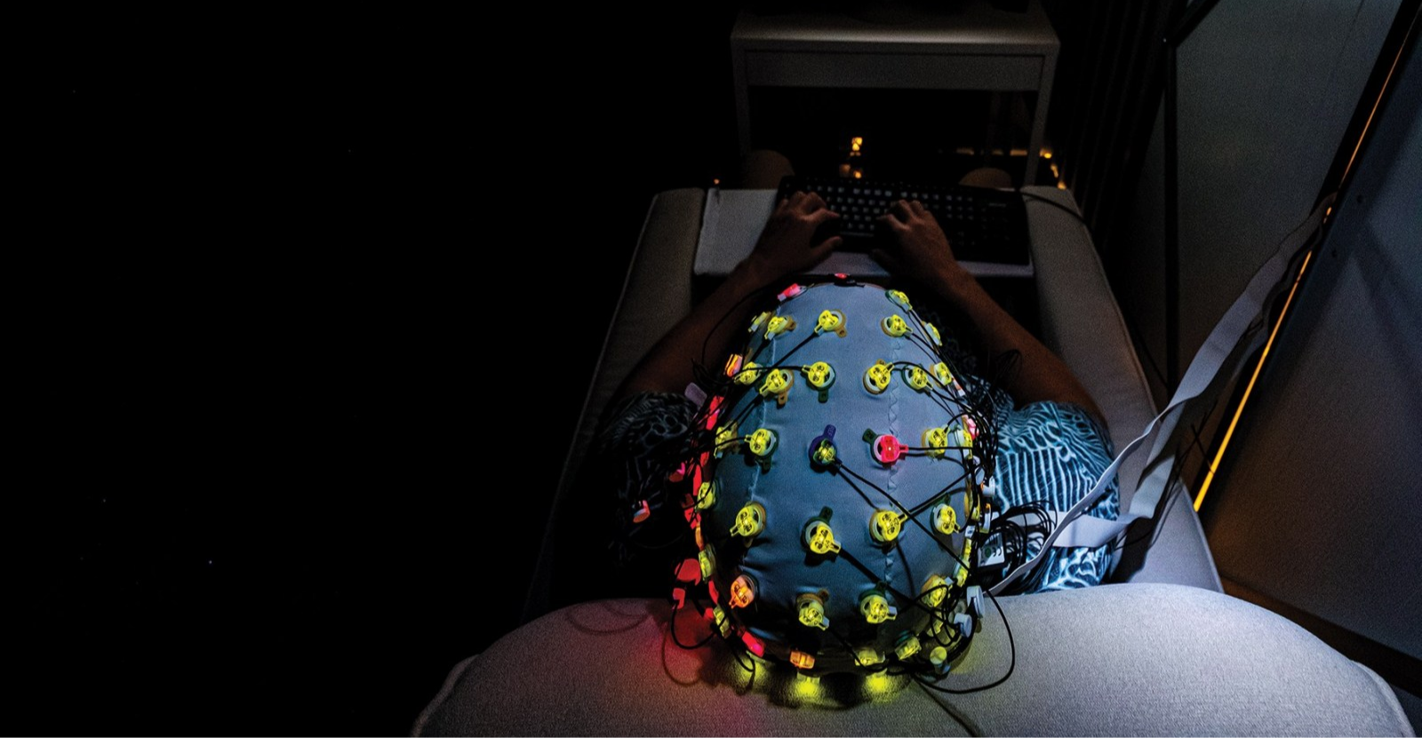
As explained in the earlier study 45 , we prepared 103 naturalistic tasks that could be performed without any pre-experimental training (see Supplementary Note  2 for the detailed description of each task). Tasks were selected to include as many cognitive domains as possible. Each task had 12 instances; 8 instances were used in the training runs, whereas 4 were used in the test runs. The stimuli were presented on a projector screen inside the scanner (21.0 × 15.8° of visual angle at 30 Hz). The root-mean square of the auditory stimuli was normalized. During scanning, subjects wore MR-compatible ear tips. The experiment was performed for 3 days, with six runs performed each day. Presentation software (Neurobehavioral Systems, Albany, CA, USA) was used to control the stimulus presentation and collection of behavioral data. To measure button responses, optic response pads with two buttons in each of the left and right hands were used (HHSC-2×2, Current Designs, Philadelphia, PA, USA).

The experiment consisted of 18 runs, with 12 training runs and 6 test runs. Each run contained 77–83 trials with a duration of 6–12 s per trial. To keep subjects attentive and engaged and to ensure all runs had the same length, a 2-s feedback for the preceding task (correct or incorrect) was presented 9–13 times per run. In addition to the task, 6 s of imaging without a task was inserted at the beginning and at the end of each run; the former was discarded in the analysis. The duration of a single run was 556 s. In the training runs, task order was pseudorandomized, as some tasks depended on each other and were therefore presented close to each other in time (e.g., the tasks “MemoryDigit” and “MatchDigit”). In the test runs, 103 tasks were presented four times in the same order across all six runs (but with different instances for each repetition). There was no overlap between the instances in the training runs and test runs. No explanation of the tasks was given to the subjects prior to the experiment. During the fMRI experiment, subjects were instructed on how to perform each task by the instruction text that was shown as a part of the stimuli. Subjects only underwent a short training session on how to use the buttons used to respond.

MRI data acquisition

The experiment was conducted using a 3.0 T scanner (TIM Trio; Siemens, Erlangen, Germany) with a 32-channel head coil. We scanned 72 interleaved axial slices that were 2.0-mm thick without a gap, parallel to the anterior and posterior commissure line, using a T2*-weighted gradient echo multiband echo-planar imaging sequence [repetition time (TR) = 2,000 ms, echo time (TE) = 30 ms, flip angle (FA) = 62°, field of view (FOV) = 192 × 192 mm 2 , resolution = 2 × 2 mm 2 , MB factor = 3]. We obtained 275 volumes for each run, with each following three dummy images. For anatomical reference, high-resolution T1-weighted images of the whole brain were also acquired from all subjects with a magnetization-prepared rapid acquisition gradient echo sequence (MPRAGE, TR = 2,530 ms, TE = 3.26 ms, FA = 9°, FOV = 256 × 256 mm 2 , voxel size = 1 × 1 × 1 mm 3 ).

fMRI data preprocessing

Motion correction in each run was performed using the statistical parametric mapping toolbox (SPM12; Wellcome Trust Centre for Neuroimaging, London, UK; http://www.fil.ion.ucl.ac.uk/spm/ ). All volumes were aligned to the first echo planar image for each subject. Low-frequency drift was removed using a median filter with a 120-s window. The slice timing correction was performed to the first slice of each scan. The response for each voxel was then normalized by subtracting the mean response and scaling it to the unit variance. We used FreeSurfer 59 , 60 to identify the cortical surfaces from the anatomical data and register them to the voxels of the functional data. For each subject, the voxels identified in the cerebral cortex (53,345–66,695 voxels per subject), cerebellum (12,505–15,262 voxels per subject), and subcortex were used in the analysis (5,384–6,622 voxels per subject). For the subcortex, voxels in the bilateral hippocampus, caudate, amygdala, accumbens, pallidum, putamen, and thalamus were included. Note that we refined preprocessing parameters (e.g., using SPM12 instead of SPM8 and adding slice timing correction) compared with our previous study 45 , which resulted in a slightly different distribution of representational similarities and decoding accuracies in the cerebral cortex.

Task-type features

The task-type features were composed of one-hot vectors, which were assigned 1 or 0 for each time bin, indicating whether one of the 103 tasks was performed in that period. The total number of task-type features was thus 103.

Encoding model fitting

In the encoding model, cortical activity in each voxel was fitted with a finite impulse response model that captured the slow hemodynamic response and its coupling with neural activity 35 , 61 . The feature matrix F E [T × 3 N] was modeled by concatenating sets of [T × N] feature matrices with three temporal delays of 2, 4, and 6 s (T = # of samples; N = # of features). The cortical response R E [T × V] was then modeled by multiplying the feature matrix F E with the weight matrix W E [3 N × V] (V = # of voxels):

We used an L2-regularized linear regression using the training dataset to obtain the weight matrix W E . The training dataset consisted of 3,336 samples (6,672 s). The optimal regularization parameter was assessed using 10-fold cross-validation, with the 18 different regularization parameters ranging from 1 to 2 17 .

The test dataset consisted of 412 samples (824 s, repeated four times). To reshape the data spanning over six test runs into the four times-repeated dataset, we discarded 6 s of the no-task period at the end of each run as well as the 2-s feedback periods at the end of the third and sixth test runs. Four repetitions of the test dataset were averaged to increase the signal-to-noise ratio. Prediction accuracy was calculated using Pearson’s correlation coefficient between the predicted signal and measured signal in the test dataset.

Evaluation of optimal regularization parameters

To keep the scale of the weight values consistent across subjects, we performed a resampling procedure to assess the optimal regularization parameter used for group RSA and PCA 38 . To this end, we randomly divided the training dataset into training samples (80%) and validation samples (20%) for each subject and performed model fitting using an L2-regularized linear regression. This procedure was repeated 50 times. The resultant prediction accuracies were averaged across the six subjects for each parameter. We selected the optimal regularization parameter that provided the highest mean prediction accuracy across subjects. This regularization parameter was used for model fitting for group RSA and PCA.

Representational similarity analysis

To examine hierarchical relations across tasks, we conducted an RSA. First, we concatenated the weight matrix of predictive voxels of the task-type model across six subjects. Concatenation of the estimated weights was performed to obtain a group-level representation that provides a common basis that is comparable across subjects 37 , 38 . To choose predictive voxels, for each subject, we selected the voxels that exhibited a significant prediction accuracy with P  < 0.05 (with FDR correction) and averaged three time delays for each task. We then obtained the RSM by calculating the Pearson’s correlation coefficients between the averaged weights of all task pairs. A dendrogram of the 103 tasks was then obtained using the task dissimilarity (1 - correlation coefficient) as a distance metric, using the minimum distance as a linkage criterion. For the purpose of visualization, tasks were reordered based on the dendrogram obtained using the cortical data.

Principal component analysis of task-type weights

For each brain region (cortex, cerebellum, or subcortex), we performed PCA on the weight matrix of the task-type model concatenated across six subjects. We selected the voxels that showed significant prediction accuracy with P  < 0.05 (with FDR correction) and averaged three time delays for each task. To show the structure of the cognitive space, 103 tasks were mapped onto the two-dimensional space using the loadings of PC1 (first PC) and PC2 as the x-axis and y-axis, respectively. The tasks were further colored in red, green, and blue based on the relative PCA loadings in PC1, PC2, and PC3, respectively.

To represent the cortical organization of the cognitive space for each subject, we extracted and normalized the PCA scores from each subject’s voxels. The resultant cortical map indicated the relative contribution of each cortical voxel to the target PC (denoted as PCA score map ).

To obtain an objective interpretation of the PCs, we performed metadata-based inference of the cognitive factors related to each PC. We used Neurosynth as a metadata reference of the past neuroimaging literature 46 . From the approximately 3,000 terms in the database, we manually selected 715 terms that covered the comprehensive cognitive factors while also avoiding redundancy. In particular, we removed several plural terms that also had their singular counterpart (e.g., “concept” and “concepts”) and past tense verbs that also had their present counterpart (e.g., “judge” and “judged”) from the dataset. We also excluded those terms that indicated anatomical regions (e.g., “parietal”). We used the reverse inference map of the Neurosynth database for each of the 715 selected terms. The reverse inference map indicated the likelihood of a given term being used in a study if the activity was observed at a particular voxel. Each reverse inference map in the MNI152 space was then registered to the subjects’ reference echo planar imaging (EPI) data using FreeSurfer 59 , 60 . For each of the PCA score maps, we calculated Pearson’s correlation coefficients with the 715 registered reverse inference maps, which resulted in a cognitive factor vector with 715 elements. Terms with higher correlation coefficient values were regarded as contributing more to the target PC.

Cognitive factor features

To obtain task representations using continuous features in the human cognitive space, we transformed sparse task-type features into latent cognitive factor feature space. We used the reverse inference map of the Neurosynth database 46 for each of the 715 terms selected. Each reverse inference map in the Neurosynth database in MNI152 space was registered to the subjects’ reference EPI data using FreeSurfer 59 , 60 .

We then calculated the Pearson’s correlation coefficients between the weight map for each task in the task-type model and the registered reverse inference maps. This resulted in the [103 × 715] coefficient matrix. We next obtained the cognitive transform function (CTF) for each subject by averaging the coefficient matrices of the other five subjects. The CTF served to transform the feature values of the 103 tasks into the 715-dimensional latent feature space. The feature matrix of the cognitive factor model was then obtained by multiplying the CTF with the feature matrix of the task-type model. Note that the CTF (and the resultant feature matrix) of each target subject was independent of their own data. The total number of cognitive factor features was 715.

Exclusion of sensorimotor voxels

To exclude the possible effect of low-level sensorimotor features on prediction and decoding performances, we performed an additional encoding model fitting using sensorimotor components. Sensorimotor features were obtained by concatenating ME features (visual), MTF features (auditory), and BR features (motor) (see the following subsections for details). Our previous studies validated the efficacy of these feature in controlling sensorimotor information 33 , 44 , 45 . Moreover, ME and MTF features are easier to interpret than neural network features because they explicitly modeled neuronal response patterns in the early visual and auditory cortices. For each subject, we randomly divided the training dataset into training (80%) and validation samples (20%) and performed model fitting using an L2-regularized linear regression. This procedure was repeated 50 times. The reliably predicted voxels by this analysis (having a mean prediction accuracy of at least 0.3) were called as sensorimotor voxels and were excluded from some of the analyses as described in the Result section.

Motion energy features

We used the ME model that has been used in previous studies 35 , 44 , 45 and provided in a public repository ( https://github.com/gallantlab/motion_energy_matlab ). First, movie frames and pictures were spatially downsampled to 96 × 96 pixels. The RGB pixel values were then converted into the Commission International de l’Eclairage (CIE) LAB color space, and the color information was subsequently discarded. The luminance (L*) pattern was passed through a bank of three-dimensional spatiotemporal Gabor wavelet filters. The outputs of the two filters with orthogonal phases (quadrature pairs) were squared and summed to yield local ME. ME was compressed with a log-transformation and temporally downsampled to 0.5 Hz. Filters were tuned to six spatial frequencies (0, 1.5, 3.0, 6.0, 12.0, 24.0 cycles per image) and three temporal frequencies (0, 4.0, 8.0 Hz), without directional parameters. Filters were positioned on a square grid that covered the screen. The adjacent filters were separated by 3.5 standard deviations of their spatial Gaussian envelopes. The total number of ME features was 1,395.

Modulation transfer function features

A sound cochleogram was generated using a bank of 128 overlapping bandpass filters ranging from 20 to 10,000 Hz. The window size was set to 25 ms and the hop size to 10 ms. The filter output was averaged across 2 s (TR). We further extracted the features from the MTF model 62 , which we provided in a public repository ( https://osf.io/ea2jc/ ). For each cochleogram, a convolution with modulation-selective filters was then calculated. The outputs of the two filters with orthogonal phases (quadrature pairs) were squared and summed to yield the local modulation energy. Modulation energy was then log-transformed, averaged across 2 s, and further averaged within each of the 10 nonoverlapping frequency ranges logarithmically spaced along the frequency axis. The filter outputs of the upward and downward sweep directions were used. Modulation-selective filters were tuned to five spectral modulation scales (0.50, 1.0, 2.0, 4.0, 8.0 cycles per octave) and five temporal modulation rates (4.0, 8.0, 16.0, 32.0, 64.0 Hz). The total number of MTF features was 1,000.

Button response features

The BR features were constructed based on the number of button responses within 1 s for each of the four buttons, with the right two buttons pressed by the right thumb and the left two buttons pressed by the left thumb. The total number of BR features was four.

Decoding model fitting

In the decoding model, the cortical response matrix R D [T × 3 V] was modeled using concatenating sets of [T × V] matrices with temporal delays of 2, 4, and 6 s. The feature matrix F D [T × N] was modeled by multiplying the cortical response matrix R D with the weight matrix W D [3 V × N]:

The weight matrix W D was estimated using an L2-regularized linear regression with the training dataset, following the same procedure for the encoding model fitting.

Decoding with novel tasks

In order to examine the generalizability of our models, we performed encoding and decoding analyses with novel tasks not used during model training (Fig.  5a ). We randomly divided the 103 tasks into five task groups. A single task group contained 20–21 tasks. We performed five independent model fittings, each with a different task group as the target. From the training dataset, we excluded the time points during which the target tasks were performed and those within 6 s after the presentation of the target tasks. In the test dataset, we used only the time points during which the target tasks were performed and those within 6 s after the presentation of the target tasks. This setting allowed us to assume that the activity induced by the target task group and that induced by the other four task groups (training task groups) did not overlap, thus enabling us to investigate prediction and decoding accuracies for novel tasks. We performed encoding and decoding model fitting with the training task group, which was composed of 82–83 tasks. For model testing, we concatenated the predicted responses or decoded features of the five task groups. Responses or features for the time points that were duplicated were then averaged across the five task groups. Note that encoding and decoding with the novel tasks were only possible with the cognitive factor model because the original tasks needed to be transformed into the latent feature space.

For the decoding analysis with novel tasks, we measured the similarity between the CTF of each task and each decoded cognitive factor vector using Pearson’s correlation coefficients for each time point. We refer to the correlation coefficient as the task score . We then calculated the time-averaged task scores for each task, and then performed decoding using the one-vs.-one method. For each target task, a series of binary classifications were performed between the target task and each of the remaining 102 tasks. The decoding accuracy was then calculated as a ratio that the target task had higher task score in this procedure. The one-vs-one decoding accuracy (ranged [0, 1], chance level = 0.5) can be considered as a standardized measure of the task score-based decoding accuracy (ranged [−1, 1], chance level = 0).

To evaluate whether the cerebellum and subcortex contain rich information to reconstruct cortical activity, we constructed additional encoding models using the cerebellar and subcortical activities as feature matrices. We first applied PCA to the original brain response matrices of the cerebellum and subcortex to reduce their dimensions to 2,000. Response matrices of the cerebellum and subcortex were independently used in the cerebellum and subcortex encoding models, respectively. For the cerebellum + subcortex encoding model, concatenated brain response matrix (totally 4,000 dimensions) was used as a feature matrix. The above encoding models were constructed and evaluated similarly as described in the encoding model fitting section.

Statistics and reproducibility

Statistical significance of encoding models (412 samples, one-sided) was computed by comparing estimated correlations with the null distribution of correlations between the two independent Gaussian random vectors with the same length as the test dataset 38 . The statistical threshold was set at P  < 0.05 and corrected for multiple comparisons using the FDR procedure 63 . The statistical significance of the decoding accuracy (for both one-vs-one and task score-based methods) was tested for each task using the one-sided sign test (102 samples; P  < 0.05, with FDR correction) 64 , which is a nonparametric statistical test used in previous decoding studies 45 , 65 , 66 , 67 . The significance of average decoding accuracy (across tasks) was further tested using the permutation test ( P  < 0.05). Specifically, task labels in the test dataset were randomly shuffled 5,000 times, and p -values were calculated (for both one-vs-one and task score-based methods) based on the resultant null distribution of average decoding accuracy. Results from the six subjects were considered as replications of the analyses. All model fitting and analyses were conducted using custom software written on MATLAB. For data visualization on the cortical maps, pycortex was used 68 .

Reporting summary

Further information on research design is available in the  Nature Portfolio Reporting Summary linked to this article.

Data availability

The raw MRI data are available at the OpenNeuro.org ( https://openneuro.org/datasets/ds002306 ) 69 . Source data underlying Figs.  2 d–f, 3 b, 4 b, 5 b–e, and 6f are provided in Supplementary Data  1 , 2 , 3 , 4 , and 5 , respectively. Other data are available from the corresponding author upon reasonable request.

Code availability

The MATLAB code for building encoding and decoding models are available at the Open Science Framework (OSF) repository associated with our previous study 45 ( https://osf.io/ea2jc/ ). Additional codes used in the current study and the datasets generated and/or analyzed during the current study are available upon request.

Roth, G. & Dicke, U. Evolution of the brain and intelligence. Trends Cogn. Sci. 9 , 250–257 (2005).

Article   PubMed   Google Scholar  

Dunbar, R. I. M. Neocortex size as a constraint on group size in primates. J. Hum. Evol. 22 , 469–493 (1992).

Article   Google Scholar  

Barton, R. A. & Venditti, C. Human frontal lobes are not relatively large. Proc. Natl Acad. Sci. U. S. A. 110 , 9001–9006 (2013).

Article   CAS   PubMed   PubMed Central   Google Scholar  

Gabi, M. et al. No relative expansion of the number of prefrontal neurons in primate and human evolution. Proc. Natl Acad. Sci. U. S. A. 113 , 9617–9622 (2016).

Azevedo, F. A. C. et al. Equal numbers of neuronal and nonneuronal cells make the human brain an isometrically scaled-up primate brain. J. Comp. Neurol. 513 , 532–541 (2009).

Barton, R. A. & Venditti, C. Rapid evolution of the cerebellum in humans and other great apes. Curr. Biol. 24 , 2440–2444 (2014).

Article   CAS   PubMed   Google Scholar  

Barger, N., Hanson, K. L., Teffer, K., Schenker-Ahmed, N. M. & Semendeferi, K. Evidence for evolutionary specialization in human limbic structures. Front. Hum. Neurosci. 8 , 277 (2014).

Article   PubMed   PubMed Central   Google Scholar  

Hori, Y. et al. Cortico-subcortical functional connectivity profiles of resting-state networks in marmosets and humans. J. Neurosci. 40 , 9236–9249 (2020).

Roberts, R. E., Bain, P. G., Day, B. L. & Husain, M. Individual differences in expert motor coordination associated with white matter microstructure in the cerebellum. Cereb. Cortex 23 , 2282–2292 (2013).

Vinueza Veloz, M. F. et al. Cerebellar control of gait and interlimb coordination. Brain Struct. Funct. 220 , 3513–3536 (2015).

Murdoch, B. E. The cerebellum and language: historical perspective and review. Cortex 46 , 858–868 (2010).

Adamaszek, M. et al. Consensus paper: cerebellum and emotion. Cerebellum 16 , 552–576 (2017).

Küper, M. et al. Cerebellar fMRI Activation Increases with Increasing Working Memory Demands. Cerebellum 15 , 322–335 (2016).

D’Mello, A. M., Gabrieli, J. D. E. & Nee, D. E. Evidence for hierarchical cognitive control in the human cerebellum. Curr. Biol. 30 , 1881–1892.e3 (2020).

Guell, X., Gabrieli, J. D. E. & Schmahmann, J. D. Triple representation of language, working memory, social and emotion processing in the cerebellum: convergent evidence from task and seed-based resting-state fMRI analyses in a single large cohort. Neuroimage 172 , 437–449 (2018).

Ashida, R., Cerminara, N. L., Edwards, R. J., Apps, R. & Brooks, J. C. W. Sensorimotor, language, and working memory representation within the human cerebellum. Hum. Brain Mapp. 40 , 4732–4747 (2019).

King, M., Hernandez-Castillo, C. R., Poldrack, R. A., Ivry, R. B. & Diedrichsen, J. Functional boundaries in the human cerebellum revealed by a multi-domain task battery. Nat. Neurosci. 22 , 1371–1378 (2019).

Keren-Happuch, E., Chen, S.-H. A., Ho, M.-H. R. & Desmond, J. E. A meta-analysis of cerebellar contributions to higher cognition from PET and fMRI studies. Hum. Brain Mapp. 35 , 593–615 (2014).

Burgess, N., Maguire, E. A. & O’Keefe, J. The human hippocampus and spatial and episodic memory. Neuron 35 , 625–641 (2002).

Zeidman, P. & Maguire, E. A. Anterior hippocampus: the anatomy of perception, imagination and episodic memory. Nat. Rev. Neurosci. 17 , 173–182 (2016).

Epstein, R. A., Patai, E. Z., Julian, J. B. & Spiers, H. J. The cognitive map in humans: spatial navigation and beyond. Nat. Neurosci. 20 , 1504–1513 (2017).

Davachi, L. & DuBrow, S. How the hippocampus preserves order: the role of prediction and context. Trends Cogn. Sci. 19 , 92–99 (2015).

Phelps, E. & Ledoux, J. Neural systems underlying emotion behavior: From animal models to human function. Neuron 48 , 175–187 (2005).

Salzman, C. D. & Fusi, S. Emotion, cognition, and mental state representation in amygdala and prefrontal cortex. Annu. Rev. Neurosci. 33 , 173–202 (2010).

FeldmanHall, O., Glimcher, P., Baker, A. L., NYU PROSPEC Collaboration & Phelps, E. A. The functional roles of the amygdala and prefrontal cortex in processing uncertainty. J. Cogn. Neurosci. 31 , 1742–1754 (2019).

Gangopadhyay, P., Chawla, M., Dal Monte, O. & Chang, S. W. C. Prefrontal–amygdala circuits in social decision-making. Nat. Neurosci. 24 , 5–18 (2020).

Saalmann, Y. B. & Kastner, S. The cognitive thalamus. Front. Syst. Neurosci. 9 , 39 (2015).

Halassa, M. M. & Kastner, S. Thalamic functions in distributed cognitive control. Nat. Neurosci. 20 , 1669–1679 (2017).

Wolff, M. & Vann, S. D. The cognitive thalamus as a gateway to mental representations. J. Neurosci. 39 , 3–14 (2019).

Bell, P. T. & Shine, J. M. Subcortical contributions to large-scale network communication. Neurosci. Biobehav. Rev. 71 , 313–322 (2016).

Naselaris, T., Kay, K. N., Nishimoto, S. & Gallant, J. L. Encoding and decoding in fMRI. Neuroimage 56 , 400–410 (2011).

Çukur, T., Nishimoto, S., Huth, A. G. & Gallant, J. L. Attention during natural vision warps semantic representation across the human brain. Nat. Neurosci. 16 , 763–770 (2013).

Nakai, T., Yamaguchi, H. Q. & Nishimoto, S. Convergence of modality invariance and attention selectivity in the cortical semantic circuit. Cereb. Cortex 31 , 4825–4839 (2021).

Kay, K. N., Naselaris, T., Prenger, R. J. & Gallant, J. L. Identifying natural images from human brain activity. Nature 452 , 352–355 (2008).

Nishimoto, S. et al. Reconstructing visual experiences from brain activity evoked by natural movies. Curr. Biol. 21 , 1641–1646 (2011).

Naselaris, T., Olman, C. A., Stansbury, D. E., Ugurbil, K. & Gallant, J. L. A voxel-wise encoding model for early visual areas decodes mental images of remembered scenes. Neuroimage 105 , 215–228 (2015).

Huth, A. G., Nishimoto, S., Vu, A. T. & Gallant, J. L. A continuous semantic space describes the representation of thousands of object and action categories across the human brain. Neuron 76 , 1210–1224 (2012).

Huth, A. G., de Heer, W. A., Griffiths, T. L., Theunissen, F. E. & Gallant, J. L. Natural speech reveals the semantic maps that tile human. Cereb. cortex. Nat. 532 , 453–458 (2016).

Google Scholar  

de Heer, W. A., Huth, A. G., Griffiths, T. L., Gallant, J. L. & Theunissen, F. E. The hierarchical cortical organization of human speech processing. J. Neurosci. 37 , 6539–6557 (2017).

Nishida, S. & Nishimoto, S. Decoding naturalistic experiences from human brain activity via distributed representations of words. Neuroimage 180 , 232–242 (2018).

Nishida, S., Blanc, A., Maeda, N., Kado, M. & Nishimoto, S. Behavioral correlates of cortical semantic representations modeled by word vectors. PLoS Comput. Biol. 17 , e1009138 (2021).

Popham, S. F. et al. Visual and linguistic semantic representations are aligned at the border of human visual cortex. Nat. Neurosci. 24 , 1628–1636 (2021).

Horikawa, T., Cowen, A. S., Keltner, D. & Kamitani, Y. The neural representation of visually evoked emotion Is high-dimensional, categorical, and distributed across transmodal brain regions. iScience 23 , 101060 (2020).

Koide-Majima, N., Nakai, T. & Nishimoto, S. Distinct dimensions of emotion in the human brain and their representation on the cortical surface. Neuroimage 222 , 117258 (2020).

Nakai, T. & Nishimoto, S. Quantitative models reveal the organization of diverse cognitive functions in the brain. Nat. Commun. 11 , 1142 (2020).

Yarkoni, T., Poldrack, R. A., Nichols, T. E., Van Essen, D. C. & Wager, T. D. Large-scale automated synthesis of human functional neuroimaging data. Nat. Methods 8 , 665–670 (2011).

LeBel, A., Jain, S. & Huth, A. G. Voxelwise Encoding Models Show That Cerebellar Language Representations Are Highly Conceptual. J. Neurosci. 41 , 10341–10355 (2021).

Van Overwalle, F., Ma, Q. & Heleven, E. The posterior crus II cerebellum is specialized for social mentalizing and emotional self-experiences: a meta-analysis. Soc. Cogn. Affect. Neurosci. 15 , 905–928 (2020).

Koziol, L. F., Budding, D. E. & Chidekel, D. From movement to thought: executive function, embodied cognition, and the cerebellum. Cerebellum 11 , 505–525 (2012).

Choi, Y., Shin, E. Y. & Kim, S. Spatiotemporal dissociation of fMRI activity in the caudate nucleus underlies human de novo motor skill learning. Proc. Natl Acad. Sci. U. S. A. 117 , 23886–23897 (2020).

Hardwick, R. M., Rottschy, C., Miall, R. C. & Eickhoff, S. B. A quantitative meta-analysis and review of motor learning in the human brain. Neuroimage 67 , 283–297 (2013).

Sherman, S. M. Thalamus plays a central role in ongoing cortical functioning. Nat. Neurosci. 19 , 533–541 (2016).

Halassa, M. M. & Sherman, S. M. Thalamocortical Circuit Motifs: A General Framework. Neuron 103 , 762–770 (2019).

Tian, Y., Margulies, D. S., Breakspear, M. & Zalesky, A. Topographic organization of the human subcortex unveiled with functional connectivity gradients. Nat. Neurosci. 23 , 1421–1432 (2020).

Anzellotti, S., Caramazza, A. & Saxe, R. Multivariate pattern dependence. PLoS Comput. Biol. 13 , e1005799 (2017).

Nishida, S. et al. Brain-mediated transfer learning of convolutional neural networks. AAAI 34 , 5281–5288 (2020).

Mell, M. M., St-Yves, G. & Naselaris, T. Voxel-to-voxel predictive models reveal unexpected structure in unexplained variance. Neuroimage 238 , 118266 (2021).

Oldfield, R. C. The assessment and analysis of handedness: the Edinburgh inventory. Neuropsychologia 9 , 97–113 (1971).

Dale, A. M., Fischl, B. & Sereno, M. I. Cortical surface-based analysis. I. Segmentation and surface reconstruction. Neuroimage 9 , 179–194 (1999).

Fischl, B., Sereno, M. I. & Dale, A. M. Cortical surface-based analysis. II: Inflation, flattening, and a surface-based coordinate system. Neuroimage 9 , 195–207 (1999).

Kay, K. N., David, S. V., Prenger, R. J., Hansen, K. A. & Gallant, J. L. Modeling low-frequency fluctuation and hemodynamic response timecourse in event-related fMRI. Hum. Brain Mapp. 29 , 142–156 (2008).

Nakai, T., Koide-Majima, N. & Nishimoto, S. Correspondence of categorical and feature-based representations of music in the human brain. Brain Behav. 11 , e01936 (2021).

Benjamini, Y. & Hochberg, Y. Controlling the false discovery rate: A practical and powerful approach to multiple testing. J. R. Stat. Soc. 57 , 289–300 (1995).

Hollander, Myles, Douglas A. Wolfe, and Eric Chicken. Nonparametric Statistical Methods.pdf. (John Wiley & Sons, 2013).

Rutishauser, U., Aflalo, T., Rosario, E. R., Pouratian, N. & Andersen, R. A. Single-Neuron Representation of Memory Strength and Recognition Confidence in Left Human Posterior Parietal Cortex. Neuron 97 , 209–220.e3 (2018).

Pereira, F. et al. Toward a universal decoder of linguistic meaning from brain activation. Nat. Commun. 9 , 963 (2018).

Sergent, C. et al. Bifurcation in brain dynamics reveals a signature of conscious processing independent of report. Nat. Commun. 12 , 1149 (2021).

Gao, J. S., Huth, A. G., Lescroart, M. D. & Gallant, J. L. Pycortex: an interactive surface visualizer for fMRI. Front. Neuroinform. 9 , 23 (2015).

Nakai, T., & Nishimoto, S. Over 100 Task fMRI Dataset. OpenNeuro. [Dataset] https://doi.org/10.18112/openneuro.ds002306.v1.0.3 . (2020)

Download references

Acknowledgements

We thank MEXT/JSPS KAKENHI (grant numbers JP17K13083 and JP18H05091 in #4903 (Evolinguistics) for T.N., JP15H05311 and JP18H05522 for S.N.) as well as JST CREST JPMJCR18A5 and ERATO JPMJER1801 (for S.N.) for the partial financial support to this study. The funders had no role in the study design, data collection and analysis, decision to publish, or preparation of the manuscript.

Author information

Authors and affiliations.

Center for Information and Neural Networks, National Institute of Information and Communications Technology, Suita, Japan

Tomoya Nakai & Shinji Nishimoto

Lyon Neuroscience Research Center (CRNL), INSERM U1028 - CNRS UMR5292, University of Lyon, Bron, France

Tomoya Nakai

Graduate School of Frontier Biosciences, Osaka University, Suita, Japan

Shinji Nishimoto

Graduate School of Medicine, Osaka University, Suita, Japan

You can also search for this author in PubMed   Google Scholar

Contributions

T.N. and S.N. designed the study; T.N. collected and analyzed the data; T.N. and S.N. wrote the manuscript.

Corresponding author

Correspondence to Tomoya Nakai .

Ethics declarations

Competing interests.

The authors declare no competing interests.

Peer review

Peer review information.

Communications Biology thanks the anonymous reviewers for their contribution to the peer review of this work. Primary Handling Editors: Stefano Palminteri, Karli Montague-Cardoso and Christina Karlsson Rosenthal.  Peer reviewer reports are available.

Additional information

Publisher’s note Springer Nature remains neutral with regard to jurisdictional claims in published maps and institutional affiliations.

Supplementary information

Peer review file, supplementary information, description of additional supplementary files, supplementary data 1, supplementary data 2, supplementary data 3, supplementary data 4, supplementary data 5, reporting summary, rights and permissions.

Open Access This article is licensed under a Creative Commons Attribution 4.0 International License, which permits use, sharing, adaptation, distribution and reproduction in any medium or format, as long as you give appropriate credit to the original author(s) and the source, provide a link to the Creative Commons license, and indicate if changes were made. The images or other third party material in this article are included in the article’s Creative Commons license, unless indicated otherwise in a credit line to the material. If material is not included in the article’s Creative Commons license and your intended use is not permitted by statutory regulation or exceeds the permitted use, you will need to obtain permission directly from the copyright holder. To view a copy of this license, visit http://creativecommons.org/licenses/by/4.0/ .

Reprints and permissions

About this article

Cite this article.

Nakai, T., Nishimoto, S. Representations and decodability of diverse cognitive functions are preserved across the human cortex, cerebellum, and subcortex. Commun Biol 5 , 1245 (2022). https://doi.org/10.1038/s42003-022-04221-y

Download citation

Received : 05 April 2022

Accepted : 03 November 2022

Published : 14 November 2022

DOI : https://doi.org/10.1038/s42003-022-04221-y

Share this article

Anyone you share the following link with will be able to read this content:

Sorry, a shareable link is not currently available for this article.

Provided by the Springer Nature SharedIt content-sharing initiative

By submitting a comment you agree to abide by our Terms and Community Guidelines . If you find something abusive or that does not comply with our terms or guidelines please flag it as inappropriate.

Quick links

• Explore articles by subject
• Guide to authors
• Editorial policies

Sign up for the Nature Briefing newsletter — what matters in science, free to your inbox daily.

Neurobehavioral Systems

Headquartered in beautiful Berkeley, California, Neurobehavioral Systems has been developing high-precision scientific software for more than two decades.

Built upon Presentation® — our flagship stimulus delivery software — we have developed the CCAB to make accurate cognitive testing accessible to all.

Meet the Team

David l. woods, phd.

CEO, Co-Founder

Peter Pebler

CTO, Co-Founder

Kristin Geraci, PhD

Director, Product

Kathleen Hall, PhD

Director, Research Operations

Isabella Jaramillo

Nate whitehill-nigl.

Office Manager

Matthew Grivich, PhD

Software Engineer

Research Associate

Mike Blank, PhD

Technical Lead

National Institutes of Health | National Institute on Aging

U.s. department of veterans affairs, university of california, davis, garrett williams.

Research Project Manager

Gabe Sucich

Emily geagan.

Matthew is a software engineer at NBS. He primarily contributes to the development and timing validation of Presentation, the stimulus engine used in the CCAB.

Matthew’s background is at the intersection of technology and science, where he develops tools that scientists can rely on to perform ground-breaking research.

After co-founding NBS, Mr. Pebler created Presentation®

— the most powerful stimulus delivery software system for neuroscience, which has advanced the research of tens of thousands of scientists around the world for 20 years. He continues to utilize his 24 years of software development experience to ensure a solid foundation for every piece of technology NBS creates.

Mr. Pebler has a BS and MS in physics, from Yale and UC Berkeley.

Mr. Kahly serves as Research Associate at NBS, where he is responsible for ensuring the smooth day-to-day operation of NBS’s research initiatives.

After finishing her degree in Cognitive Psychology at UC Santa Cruz, Dr. Geraci joined NBS as a Content Developer in 2005. She has learned and grown with the company, honing her research skills, programming, and business acumen to become Director of Product.

Dr. Geraci has overseen the addition of myriad Presentation features over the years and continues to innovate with the development of CCAB testing and advanced data analysis.

Dr. Hall joined NBS as the Research Operations Director in 2021, and oversees research initiatives and the development of the CCAB.

During her graduate studies in linguistics at Northwestern University, Dr. Hall obtained extensive training in conducting behavioral experiments, with a focus on psycholinguistics and the representation and processing of syntactic constraints. Currently, Dr. Hall is focused on making cognitive testing more accessible to under-served populations, including leading translation initiatives to bring the CCAB to speakers of varied languages.

Dr. Woods is a co-founder and CEO of NBS who has helped direct the development of Presentation® software for the past 20 years.

During Dr. Woods’s long research career in cognitive neuroscience at UC Davis and the VA, he developed early versions of selected CCAB tests.

In 2017, Dr. Woods moved to NBS where he is currently CEO and the PI on an NIA-funded SBIR grant that supports normative data collection using redesigned CCAB tests that incorporate consensus ASR, neural text-to-speech, and tele-medical control through the CCAB Examiner interface.

An official website of the United States government

The .gov means it’s official. Federal government websites often end in .gov or .mil. Before sharing sensitive information, make sure you’re on a federal government site.

The site is secure. The https:// ensures that you are connecting to the official website and that any information you provide is encrypted and transmitted securely.

• Publications
• Account settings

Preview improvements coming to the PMC website in October 2024. Learn More or Try it out now .

• Advanced Search
• Journal List

OpenSesame: An open-source, graphical experiment builder for the social sciences

Sebastiaan mathôt.

Department of Cognitive Psychology, Vrije Universiteit, Van der Boechorststraat 1, 1081 HV Amsterdam, The Netherlands

Daniel Schreij

Jan theeuwes.

In the present article, we introduce OpenSesame, a graphical experiment builder for the social sciences. OpenSesame is free, open-source, and cross-platform. It features a comprehensive and intuitive graphical user interface and supports Python scripting for complex tasks. Additional functionality, such as support for eyetrackers, input devices, and video playback, is available through plug-ins. OpenSesame can be used in combination with existing software for creating experiments.

Introduction

A little over 20 years ago, Schneider ( 1988 ) estimated that it took a professional programmer approximately 160 h to implement a new experimental paradigm. Fortunately, things have changed since then. Advances in both software and hardware have made it possible for unskilled programmers to develop their experiments rapidly, using any of the available “point-and-click” software packages (for a comparison, see Stahl, 2006 ). Scientists who prefer programming over the use of a graphical interface also benefit from the power of modern, high-level programming languages, which have substantially improved the readability and reduced the amount of code required to perform most tasks.

Another important development is the increased availability of high-quality, free experimental software. Currently, there are at least eight free software packages that are viable tools for creating experiments (see Table  1 ). However, these packages occupy a relatively small niche, mostly because they do not offer the type of fully graphical interface that many users have come to expect. Therefore, researchers who are most comfortable in a graphical environment generally use proprietary software.

An overview of software for creating experiments

* Source-code is not available

** Depends on MATLAB (The MathWorks, 1998 ), a proprietary software package, for full functionality. Offers limited support for Octave (Eaton, 2002 ), an open-source MATLAB clone

*** Uses a form-based interface

**** Offers limited support for Mac OS and Linux

In the present article, we introduce OpenSesame, a new experiment builder. OpenSesame is unique in that it is free, cross-platform, and arguably, offers the most intuitive and comprehensive graphical user interface (GUI) currently available. For complex tasks, which cannot be performed through the GUI, OpenSesame supports Python scripting (Van Rossum & Drake, 2011 ). A wide range of experiments can be created, including psychophysical experiments, speeded response time tasks, eye-tracking studies, and questionnaires.

In the first section of the present article, we provide a nontechnical description of the functionality offered by OpenSesame. In the second section, we describe how OpenSesame compares with, and can be used in combination with, existing software. The third section deals with timing considerations and is followed by the fourth section, in which the results of a benchmark experiment are described.

OpenSesame is freely available for download from http://www.cogsci.nl/opensesame . Documentation, a step-by-step tutorial, example experiments, and plug-ins can be found in the documentation area at http://osdoc.cogsci.nl/ . The version of OpenSesame reviewed in the present article is 0.24. At the time of writing, OpenSesame has been downloaded more than 10,000 times (nonunique downloads from cogsci.nl and via bit-torrent), and there is an active support forum.

Usage and functionality

System requirements.

OpenSesame does not impose strict system requirements. Installation packages are available for Windows XP/Vista/7 and Ubuntu/Debian Linux. OpenSesame has been extensively tested on those platforms. At the time of writing, packages for Mac OS are also available but have been labeled “experimental” pending further testing. On other platforms, users will need to manually install the software on which OpenSesame depends and run OpenSesame from the source code. Instructions for running OpenSesame from source are provided online.

The processing power required to run OpenSesame depends strongly on the type of experiment. For a typical experiment, consisting of a sequence of static stimulus displays followed by response collection, the requirements are very modest, and any relatively modern computer system will suffice (we have successfully run OpenSesame on a low-end netbook; 2-GB Ram, 1.66-GHz Intel Atom N270). When using complex stimuli, such as high-definition video, the user will need to evaluate for him- or herself whether the computer system is up to the task.

The graphical user interface

After starting OpenSesame, the user is presented with a GUI (see Fig.  1 ). The structure of the experiment is depicted graphically as a tree structure in the overview area (Fig.  1b ). An experiment consists of a collection of items , which are self-contained parts of the experiment (i.e., conceptually distinct units). Items can be added to the experiment by dragging them from the item toolbar (Fig.  1a ) onto the overview area. Items can be edited by selecting them in the overview area, after which the appropriate controls appear in the tab area (Fig.  1c ).

The OpenSesame graphical user interface on start-up. a The item toolbar contains icons that can be dragged into the overview area. b The overview area represents the experiment as a tree-structure. c The tab area contains tabs for editing items and getting context-sensitive help. By clicking on an item in the overview area, a tab with the appropriate controls opens. By clicking on one of the blue “help” buttons, a context-sensitive help tab opens. d The structure of an example experiment shown in the overview area

There are 10 core items that provide the basic functionality for creating an experiment (see Table  2 for an overview; functionality can be extended as described in the Usage and functionality: Plug-ins section). Examples of items are the sketchpad , which handles the presentation of a single stimulus display, and the keyboard_response , which handles the collection of a single keyboard press. Two special items are the loop and the sequence , which control the structure of the experiment. A sequence item sequentially calls a number of other items. A loop item repeatedly calls a single other item, while varying the values of independent variables. By combining items in various ways, arbitrary experimental paradigms can be constructed (Fig.  1d ).

An overview of the 10 core items

Variables and conditional (“if”) statements

One of the biggest challenges when designing a GUI is to offer sufficient flexibility. In OpenSesame, this flexibility is achieved through the support of variables and conditional (“if”) statements.

Variables can be built in (e.g., subject_nr ), set by items (e.g., response_time , which is set by keyboard_response items), or specified by the user in loop items (see Fig.  2a ). These variables can be used throughout the GUI, by entering [variable_name] in places where you would normally encounter a static value. For example, if the user has defined a variable called SOA , this variable can be used to control the duration of a sketchpad item (i.e., a stimulus display) by entering [SOA] in the duration field (Fig.  2b ). Analogously, feedback of the average response times can be given by adding the text “Your average response time was [avg_rt]msg” to a feedback item (Fig.  2c ).

Using variables and conditional (“if”) statements. a Independent variables can be defined in a loop item. b By entering [SOA] in the duration field of a sketchpad item, the variable SOA is used to control the presentation duration of the sketchpad. This assumes that SOA has been defined elsewhere in the experiment. c By using [avg_rt] and [acc] as part of the text in a feedback item, appropriate feedback can be given to the user. The variables avg_rt and acc are set automatically by the various response items (e.g., keyboard_response ). d Conditional statements can be used to control which items from a sequence will be called. By entering [correct] = 1 in the “Run if…” field of “green_fixation,” the item will be called only if the variable correct has been set to 1 . The variable correct is set automatically by the various response items

Particularly powerful is the possibility of combining the what-you-see-is-what-you-get sketchpad drawing tool (shown in Fig.  2b, c ) with the use of variables. The drawing tool automatically generates a simple script that defines the elements in the sketchpad . By replacing the static coordinates, colors, sizes, and so forth with variables, the user can create a flexible stimulus display in an intuitive way. For example, if you insert an image (from the file fork_left.png ) in the center of the display, OpenSesame will generate the following line of script (taken from the affordances_orientation example experiment, available online):

By right clicking on the object, you are given the possibility of editing this line. The static values can be replaced by variables, and thus the presented image, as well as the image's size, can be made variable (this will result in the object being hidden from the drawing tool, with the message that the sketchpad contains a variably defined object):

Conditional statements, commonly referred to as “if” statements, can be used to add even more flexibility to the GUI. Every item from a sequence item has a “Run if” parameter that is evaluated before the item is called. This can be used, for example, to show a green or red fixation dot, depending on whether the preceding response was correct (using the correct variable, which is automatically set by response items; see Fig.  2d ). Analogously, in sketchpad and feedback items, conditional statements can be used to control which elements are actually shown, by setting the “Show if” parameter.

Data output format

Usually, data logging will be handled by the logger item. Every time that a logger item is called, a single row of data is written to the output file. The output file is a plain-text comma-separated spreadsheet (.csv), in which each row typically corresponds to a trial and each column corresponds to a variable. This format is compatible with all commonly used spreadsheet software.

Alternatively or in addition, users can write arbitrary messages to the output file, using Python code in inline_script items. In this case, the format of the output file is determined by the user.

Python inline coding

Despite the flexibility of the GUI, there will sometimes be situations that require a full-fledged programming language. For this reason, OpenSesame supports Python scripting (Van Rossum & Drake, 2011 ). Python is a powerful programming language that is widely used in the scientific community and the computing world in general (the seventh most widely used programming language, according to Tiobe.com, 2011 ).

To use Python scripting, you add an inline_script item to the experiment. Rather than the knobs, buttons, and input fields that you will see when editing other items, the inline_script item offers an embedded programming editor. You can use the OpenSesame Python modules, which offer simple routines for handling display presentation, sound generation, response collection, and so forth. Alternatively, you can interact directly with the selected back-end (see the Usage and functionality: The back-end layer section). The latter option is mostly useful for advanced users who are familiar with one of the back-ends (i.e., PsychoPy [Peirce, 2007 ], PyGame, and/ or OpenGL) or if the native OpenSesame modules do not offer the desired functionality.

File format and the file pool

External files, such as images, sound files, and videos, are stored in the file pool (Fig.  3 ). Optionally, OpenSesame also copies participant data files to the file pool after an experiment has finished. The file pool is saved along with the experiment in a single .opensesame.tar.gz file. This extension is somewhat ungainly but accurately reflects that the file is a .tar.gz archive, which can be opened in most archiving tools (e.g., WinRar or FileRoller). Therefore, in the unlikely event that OpenSesame fails to open the experiment, you can still access the experiment script and any files that have been stored in the file pool.

The file pool. All files that are used in the experiment, such as images, sounds, and videos, are stored in the file pool. The file pool is saved along with the experiment, allowing for maximum portability

OpenSesame can be extended through plug-ins. Plug-ins offer graphical controls, appear in the item toolbar, and can be dragged into the experiment just like the built-in items. Therefore, from the perspective of the user, there is little difference between using a plug-in and using any of the 10 core items.

Plug-ins offer arbitrary functionality, such as support for specific devices or handling particular tasks that would otherwise have to be implemented through Python inline code. Currently, there are plug-ins available that support the Eyelink series of eyetrackers (SR Research, Mississauga, ON, Canada), the Mantra object tracker (Mathôt & Theeuwes, 2011 ), the Serial Response Box (Psychology Software Tools, Sharpsburg, PA), input devices connected to the parallel port, and video playback.

The back-end layer

OpenSesame consists of three distinct layers. The top layer handles the GUI and offers the functionality needed to create an experiment. The middle layer handles the execution of an experiment. The bottom, or back-end, layer handles the interaction with the display, sound, and input devices.

There are many different Python libraries available that could, in principle, be used in the back-end layer. Some, such as PyGame, Pyglet, and PyOpenGL, are general purpose, mostly oriented toward development of games. Others, such as PsychoPy (Peirce, 2007 ), VisionEgg (Straw, 2008 ), and PyEPL (Geller, Schleifer, Sederberg, Jacobs, & Kahana, 2007 ), have been developed specifically for creating psychological experiments.

OpenSesame is back-end independent, in the sense that different libraries can be used in the back-end layer. New back-ends can be created and added, much like plug-ins. Currently, there are three back-ends available: the legacy back-end, which uses PyGame; the psycho back-end, which uses PsychoPy (Peirce, 2007 ); and the opengl back-end, which uses PyGame in combination with PyOpenGL (see Table  3 ).

An overview of OpenSesame back-ends

From the perspective of the GUI user, there is little noticeable difference between the back-ends (although there may be small differences in anti-aliasing and font rendering). A red square will always be a red square, regardless of which library is used to draw it. Nevertheless, there are compelling reasons for having different back-ends to choose from. The first is that not all back-ends may be equally well supported on all platforms. Second, back-ends may differ in their timing properties (see the Benchmark experiment section). Third, each back-end offers unique functionality that the user can exploit when writing Python inline code. For example, if the psycho back-end is enabled, you can use the PsychoPy routines for creating visual stimuli. More generally, users can select the back-end that they are most familiar with and best suits their own approach to creating experiments.

Comparison with and interoperability with existing software

Table  1 provides a list of the most popular software for creating experiments. There are already many software packages to choose from, yet the functionality offered by OpenSesame is unique. In this section, we will focus on two packages with which OpenSesame arguably has the most in common: E-Prime (Psychology Software Tools, Sharpsburg, PA) and PsychoPy (Peirce, 2007 ).

E-Prime has been built on the legacy of the Micro Experimental Library (MEL; Schneider, 1988 ). Largely because it was one of the first programs to offer a graphical environment for creating experiments, E-Prime has, in our experience, become the de facto standard in many psychological labs around the world. There are at least four important differences between E-Prime and OpenSesame. The most obvious difference is that OpenSesame is free and open-source, whereas E-Prime is nonfree and proprietary. Because of the open character of OpenSesame and the availability of a plug-in framework, it is easy for third parties to add and modify functionality. Second, OpenSesame is cross-platform, whereas E-Prime is exclusively available for Windows. A final, crucial difference is the language that is used for inline coding. Whereas E-Prime uses E-Basic, a dialect of the well-known BASIC language, OpenSesame uses Python (see the Usage and functionality: Python inline coding section). The advantage of using Python over E-Basic is the availability of a large number of libraries, many of which are oriented toward the scientific community (e.g., Jones, Oliphant, & Peterson, 2001 ).

PsychoPy is an open-source project that has gained considerable momentum as a comprehensive and well-maintained Python library for creating psychological experiments (Peirce, 2007 ). Like OpenSesame, PsychoPy is cross-platform and open-source. And like OpenSesame, PsychoPy offers both a GUI (the “builder view”) and a set of Python libraries. However, there are substantial differences between the graphical interfaces offered by both packages. In the builder view of PsychoPy, the temporal progression of the experiment is shown, but the spatial arrangement of the stimuli is not readily apparent. In OpenSesame, the temporal progression is shown as well (in the overview area; see Fig.  1b, d ), but in addition, the user can get a visual preview of the stimulus arrangements through the sketchpad item (Fig.  1c ). Depending, of course, on the prior experience and personal preference of the user, such a preview can be very helpful. OpenSesame also offers a number of advanced features, which are not available in the PsychoPy builder view, such as integrated drawing tools, a more advanced sound synthesizer, and GUI support for widely used devices such as the Serial Response Box (Psychology Software Tools, Sharpsburg, PA) and the Eyelink series of eyetrackers (SR Research, Mississauga, ON, Canada). More generally, OpenSesame and PsychoPy differ in their target audience and core functionality. Although PsychoPy provides a GUI, the focus is on the specialized set of Python libraries, which offer high-level routines for creating complex visual stimuli, particularly those that are frequently used in psychophysical experiments (e.g., Gabor patches and random dot patterns). For this reason, PsychoPy will appeal mostly to people who prefer to code their experiments, such as MATLAB users who are looking for a viable open-source alternative. In contrast, OpenSesame offers only basic Python libraries but has a comprehensive GUI and will, therefore, appeal to users who are mostly at home in a graphical environment. As was discussed previously (see the Usage: The back-end layer section), OpenSesame and PsychoPy can be used in combination. This allows users to get “the best of both worlds” by combining the OpenSesame GUI with the PsychoPy Python libraries.

What is “millisecond precision timing”?

A common and valid question that applies to all experiment-building software is whether the timing is sufficiently precise. In our view, the best measure of a system's timing precision is the interval between the timestamp of a stimulus' presentation and the timestamp of a response, given the fastest possible responder that is not directly part of the system itself. Put more simply, the lowest possible response time is a good indication of a system's timing precision. The reason for this is that any inaccuracies in the timing of display presentation and response collection will add to the lowest possible response time. Perhaps even more importantly, the lowest possible response time should be consistent, so that any delay is fixed and does not constitute a source of noise (see also the Benchmark experiment section).

However, even when a system has “millisecond precision timing” in this sense, as most modern systems do, there are other factors that should be taken into account. First, many psychological labs, including our own, often use garden variety keyboards as input devices. Such keyboards have been designed to keep up with typing, and not to record responses with millisecond precision. As such, keyboards have been reported to have a relatively high and variable latency of up to 20 ms (however, it is debatable whether this constitutes a significant source of noise, when the much larger variability in human response times is considered; for a discussion, see Damian, 2010 ).

Computer monitors also have a number of peculiar properties. Rather than being refreshed instantaneously, monitors are refreshed line by line from the top down and, for each line, pixel by pixel from left to right. On CRT (nonflat screen) monitors, there is only a single active pixel at any given time, so pixels are “fading out” most of the time (which is why you can observe a flickering at low refresh rates). On TFT (flat screen) monitors, pixels remain active, so a refresh resembles a “flood fill” from top to bottom (which is why you do not observe flickering on a TFT monitor). Most researchers are aware that it is best to synchronize the presentation of a new display with the moment that the monitor starts refreshing from the top ( synchronization to vertical refresh , or v-sync ). However, even if this is done, displays do not appear instantaneously. With a refresh rate of 100 Hz, a stimulus presented at the top of the display will appear up to 10 ms before a stimulus presented at the bottom of the display. Another consequence of the monitor's refresh cycle is that displays cannot be presented at arbitrary points in time. Again, with a refresh rate of 100 Hz, the interval between two stimulus displays is always a multiple of 10 ms. Attempting to use different intervals will lead to dropped frames or aberrant timing.

The prepare–run strategy

Psychological experiments typically consist of short intervals, called trials , during which a participant perceives stimuli and performs a task. Timing should be controlled during a trial, but some unpredictable variation in the duration of the interval between trials is acceptable (cf. Schneider, 1988 ). Therefore, the best strategy for experimental software is to perform time-consuming tasks before a trial and to keep the operations that need to be performed during a trial to a bare minimum.

OpenSesame implements this strategy by calling each element from a sequence item twice. During the prepare phase, items are given time to prepare—for example, by generating a sound in the case of a synth item, or by creating an “offline canvas” in the case of a sketchpad . During the run phase, items simply execute a very limited number of trivial functions, such as showing a previously constructed canvas. This strategy substantially reduces the risk of timing glitches. The prepare–run strategy is implemented at the level of sequence items, which will typically contain the time-critical parts of an experiment. If a sequence is called multiple times by a loop , the loop as a whole is not prepared. Doing so would quickly lead to excessive memory usage and potentially cause, rather than prevent, timing issues.

Testing your own system

The timing properties of OpenSesame, or any other experiment builder, depend on the computer setup that is used. Therefore, OpenSesame comes with a basic test experiment ( test_suite ) that allows you to run a number of checks. Most importantly, the test experiment checks whether the reported interval between two presented sketchpads matches the specified interval. The same test allows you to verify that synchronization to the vertical refresh is enabled (see the Timing: What is “millisecond precision timing”? section). If not, “tearing,” in the form of horizontal lines running through the display, will be readily apparent.

Benchmark experiment

Even though the included test experiment allows you to run some useful checks (see the Timing: Testing your own system section), it is important to note that this form of testing relies on the computer's self-report. And this can be misleading. Specifically, the computer may report that a display has been presented when, in fact, it has only been queued and will be presented some time later. The aim of the present experiment was, therefore, to check timing precision more rigorously and to provide a list of benchmarks that allow the reader to evaluate whether OpenSesame is sufficiently precise to be useful in his or her experimental setting.

We used an artificial responder that responds, for all intents and purposes, instantaneously to an increase in light intensity. We measured the response times to a white display. Both inaccuracies in the reported time of display presentation (assuming that inaccuracies are always such that the display is presented after the reported time, and never before) and inaccuracies in the reported time of the response (assuming that inaccuracies are always such that the reported time of the response is after the actual response) add to the lowest possible response time. The lowest possible response time can therefore be used as a measure of the combined timing precision of display presentation and response collection.

Two different test systems were used (the system specifications are listed in Table  4 ). A black display was presented for 100 ms, followed by a white display. Automated responses to the white display were collected using a modified button-box that responds to an increase in light intensity (i.e., the presentation of the white display) through a photo-resistor. This photo-resistor was attached to the top-left of the monitor. To ensure that we obtained realistic results (i.e., not tweaked to optimize performance), the test experiment was created entirely using the GUI, and no Python inline code was used. The serial response box plug-in was used to interface with the button-box.

Results of the benchmark experiment

* Computer: Intel Core 2 DUO E8400, 3Ghz, 2Gb; graphics adapter: ATI Radeon EA H4350 (discrete); monitor: Samsung 2233RZ, TFT, 22 in

** Computer: Intel Core 2 DUO E8400, 3Ghz, 2Gb; graphics adapter: Intel GMA 4500, Intel Q45/Q43 Express chipset (integrated); monitor: Llyama vision master pro 454, CRT, 17 in

*** Running Gnome 2.30 with the Metacity window manager. The compositing layer (i.e., “Compiz” or “Desktop Effects”) was disabled

The experiment was run under Windows XP (Systems 1 and 2) and Ubuntu Linux 10.04 (System 2). The following combinations of resolution and refresh rate were tested: 1,680 × 1,050 at 120 Hz (System 1); 1,280 × 1,024 at 85 Gz (System 2); 1,024 × 768 at 60 Hz (System 2). A color depth of 32 bits was used in all cases. All three currently available back-ends were tested: legacy , opengl (Linux only), and psycho (see the Usage and functionality: The back-end layer section). For each test, 1,000 responses were collected. During the test, we checked visually for “tearing,” which indicates that the synchronization to the vertical refresh is not enabled.

Results and discussion

The results of the experiment are shown in Fig.  4 and, in more detail, in Table  4 . No further statistics were performed, since the data are essentially descriptive. Synchronization to the vertical refresh was enabled in all cases except for the legacy back-end on Ubuntu Linux 10.04. The results clearly show that for time-critical experiments, it is advisable to use one of the hardware accelerated back-ends, either psycho or opengl . With these, the response times are consistently below 4 ms on Windows XP and 2 ms on Ubuntu Linux 10.04. This negligible delay should be acceptable in even the most time-critical experiments.

Results of the benchmark experiment. The automated response times are shown as a Tukey box plot conform Robbins ( 2004 ). The central line reflects the median value. The rectangle shows the interquartile range (the 25th percentile to the 75th percentile). The whiskers reflect the minimum and maximum values that fall within 1.5 times the interquartile range. Dots correspond to individual observations that fall outside of 1.5 times the interquartile range

As an aside, the results do not show any evidence that display mode has an impact on performance (preparing a large canvas obviously takes more time, but this cost is hidden in the prepare phase, as is discussed in the Timing: The prepare–run strategy section). This means that there is no reason to choose a low resolution, color depth, or refresh rate, unless many of the drawing operations are performed “on the fly,” rather than prepared beforehand.

In the present article, we have introduced OpenSesame, a graphical, open-source experiment builder for the social sciences. OpenSesame complements existing experiment-building software in a number of ways.

First, OpenSesame offers the kind of fully graphical environment that, until now, was offered only by proprietary, nonfree software.

Second, OpenSesame is extensible through plug-ins (see the Usage and functionality: Plug-ins section). Among other things, this means that support for external devices can be added and, once a plug-in has been created, this novel functionality will integrate seamlessly with the user interface. Currently available plug-ins offer support for the Eyelink series of eyetrackers (SR Research, Mississauga, ON, Canada), the Mantra object tracker (Mathot & Theeuwes, 2011 ), the Serial Response Box (Psychology Software Tools, Sharpsburg, PA), input devices connected to the parallel port, and video playback.

Third, OpenSesame supports Python scripting (see the Usage and functionality: Python inline coding section). Even though the aim of OpenSesame is to have a flexible user interface that allows you to create complex experimental paradigms in a graphical way, there will sometimes be occasions where there is a need for a full programming language. Python (Van Rossum & Drake, 2011 ) is a widely used language and has excellent support for scientific applications in general (Jones et al., 2001 ) and for the design of psychological experiments in particular (Geller et al., 2007 ; Peirce, 2007 ; Straw, 2008 ).

Fourth, OpenSesame aims for interoperability with existing software. Specifically, this means that OpenSesame can use different back-ends to handle display and input operations (see the Usage and functionality: The back-end layer section). If, for example, you want to use the PsychoPy (Peirce, 2007 ) routines for creating visual stimuli, you can select the psycho back-end. When this back-end is selected, all display and input operations will be handled by PsychoPy, and you will be able to use the PsychoPy routines in your experiment. Other back-ends can be created and added in much the same way as plug-ins.

Fifth, OpenSesame is cross-platform (see the Usage and functionality: System requirements section). This is particularly useful in environments where different operating systems are being used. For example, our own lab contains a mixture of Windows XP, Mac OS, and Linux computers. With OpenSesame, experiments are fully portable between operating systems.

In summary, OpenSesame is a new graphical experiment builder for the social sciences. OpenSesame is unique in that it makes creating psychological experiments easy and accessible for everyone. And perhaps even fun.

Author Note

We would like to thank Per Sederberg for his code contributions (opengl back-end and advanced_delay plug-in), Jarik den Hartog and Cor Stoof for their technical support, the NeuroDebian team (Michael Hanke and Yaroslav Halchenko) for their expertise in Debian packaging, and Lotje van der Linden for her ideas and help with the tutorial. This research was funded by Netherlands Organization for Scientific Research Grant 463-06-014 to Jan Theeuwes.

Open Access

This article is distributed under the terms of the Creative Commons Attribution Noncommercial License which permits any noncommercial use, distribution, and reproduction in any medium, provided the original author(s) and source are credited.

• Brainard DH. The psychophysics toolbox. Spatial Vision. 1997; 10 :433–436. doi: 10.1163/156856897X00357. [ PubMed ] [ CrossRef ] [ Google Scholar ]
• Cohen JD, MacWhinney B, Flatt M, Provost J. PsyScope: An interactive graphic system for designing and controlling experiments in the psychology laboratory using Macintosh computers. Behavior Research Methods, Instruments, & Computers. 1993; 25 :257–271. doi: 10.3758/BF03204507. [ CrossRef ] [ Google Scholar ]
• Damian MF. Does variability in human performance outweigh imprecision in response devices such as computer keyboards? Behavior Research Methods. 2010; 42 :205–2011. doi: 10.3758/BRM.42.1.205. [ PubMed ] [ CrossRef ] [ Google Scholar ]
• Eaton JW. GNU Octave manual. Bristol, U.K.: Network Theory Ltd.; 2002. [ Google Scholar ]
• Forster KI, Forster JC. DMDX: A windows display program with millisecond accuracy. Behavior Research Methods, Instruments, & Computers. 2003; 35 :116–124. doi: 10.3758/BF03195503. [ PubMed ] [ CrossRef ] [ Google Scholar ]
• Geller AS, Schleifer IK, Sederberg PB, Jacobs J, Kahana MJ. PyEPL: A cross-platform experiment-programming library. Behavior Research Methods. 2007; 39 :950–958. doi: 10.3758/BF03192990. [ PMC free article ] [ PubMed ] [ CrossRef ] [ Google Scholar ]
• Jones, E., Oliphant, T., & Peterson, P. (2001). Scipy: Open source scientific tools for Python . Retrieved from http://www.scipy.org/
• Mathôt, S., & Theeuwes, J. (2011). Mantra: An open method for object and movement tracking. Behavior Research Methods . doi:10.3758/s13428-011-0105-9 [ PMC free article ] [ PubMed ]
• The MathWorks. (1998). MATLAB user's guide. Natick, MA: Author
• Mueller, S. T. (2010). The PEBL manual . Retrieved from http://pebl.sourceforge.net/
• Peirce JW. PsychoPy: Psychophysics software in Python. Journal of Neuroscience Methods. 2007; 162 :8–13. doi: 10.1016/j.jneumeth.2006.11.017. [ PMC free article ] [ PubMed ] [ CrossRef ] [ Google Scholar ]
• Robbins NB. Creating more effective graphs. 1. Hoboken, NJ: Wiley-Interscience; 2004. [ Google Scholar ]
• Schneider W. Micro experimental laboratory: An integrated system for IBM PC compatibles. Behavior Research Methods, Instruments, & Computers. 1988; 20 :206–217. doi: 10.3758/BF03203833. [ CrossRef ] [ Google Scholar ]
• Stahl C. Software for generating psychological experiments. Experimental Psychology. 2006; 53 :218–232. doi: 10.1027/1618-3169.53.3.218. [ PubMed ] [ CrossRef ] [ Google Scholar ]
• Stevens M, Lammertyn J, Verbruggen F, Vandierendonck A. Tscope: A C library for programming cognitive experiments on the MS Windows platform. Behavior Research Methods. 2006; 38 :280–286. doi: 10.3758/BF03192779. [ PubMed ] [ CrossRef ] [ Google Scholar ]
• Stoet G. PsyToolkit: A software package for programming psychological experiments using Linux. Behavior Research Methods. 2010; 42 :1096–1104. doi: 10.3758/BRM.42.4.1096. [ PubMed ] [ CrossRef ] [ Google Scholar ]
• Straw AD. Vision Egg: An open-source library for realtime visual stimulus generation. Frontiers in Neuroinformatics. 2008; 2 (4):1–10. [ PMC free article ] [ PubMed ] [ Google Scholar ]
• Tiobe.com. (2011, May). Most popular programming languages. Retrieved from http://www.tiobe.com/index.php/content/paperinfo/tpci/index.html
• Van Rossum G, Drake FL. Python language reference manual. Bristol, U.K.: Network Theory Ltd.; 2011. [ Google Scholar ]

If you have never used Presentation or created an account on this site before, you can try Presentation for 30 days for free. This trial license will allow you to run the same version of Presentation that you would with a purchased license. After the trial license has expired, we hope Presentation is suitable for your needs and that you would like to purchase a license.

Please contact us if you need more time to evaluate Presentation. If you still have questions about Presentation's capabilities that you were unable to answer while using the trial license, you can ask questions on our Forums .