

Excel Tutorial: How To Annotate A Graph In Excel
Introduction.
When it comes to presenting data in Excel, annotating graphs can make a world of difference. Not only does it add clarity and context to your visualizations, but it also helps to highlight key insights and trends. In this tutorial, we'll explore the different ways you can annotate a graph in Excel to create clear and effective data visualizations.
Key Takeaways
- Annotations in Excel are crucial for adding clarity and context to data visualizations.
- There are various types of annotations that can be added to a graph in Excel, including text, shapes, arrows, and data labels.
- Best practices for effective graph annotations include keeping them clear and concise, using them to highlight key insights, and avoiding clutter.
- Advanced annotation techniques in Excel include utilizing trendlines, error bars, callouts, leader lines, and dynamic annotations.
- Reviewing and editing annotations in Excel is important for ensuring the accuracy and effectiveness of data visualizations.
Understanding Graph Annotations in Excel
When working with graphs in Excel, it's important to understand how to effectively annotate your data to provide context and clarity. This tutorial will guide you through the process of adding annotations to your graphs in Excel.
Define what graph annotations are
Graph annotations are visual elements, such as text, shapes, or lines, that are added to a graph to provide additional information or context. They help to highlight key points, trends, or outliers within the data, making it easier for the reader to interpret the graph.
Explain the various types of annotations that can be added to a graph in Excel
Excel provides a range of tools for adding annotations to your graphs, including:
- Data labels: These are used to display the exact values of data points on the graph.
- Text boxes: These allow you to add custom text to the graph to provide explanations or additional information.
- Shapes and lines: These can be used to draw attention to specific areas of the graph, such as trend lines or highlighting a particular data point.
Provide examples of when and why annotations are useful for data interpretation
Annotations are useful in a variety of scenarios, such as:
- Highlighting specific data points or outliers that require further explanation.
- Providing context for trends or patterns within the data.
- Explaining any unusual variations or discrepancies in the data.
By adding annotations to your graphs in Excel, you can enhance the clarity and interpretability of your data, making it easier for others to understand and draw insights from the information you are presenting.
Step-by-Step Guide to Annotating a Graph in Excel
Annotating a graph in Excel is a useful feature that allows you to add text, shapes, arrows, and data labels to your graph to emphasize important points or trends. Here’s a step-by-step guide on how to annotate a graph in Excel.
How to add text annotations to a graph
- Click on the graph to select it.
- Go to the “Insert” tab and click on “Text Box.”
- Click and drag to draw a text box on the graph, then type your annotation.
- You can resize and reposition the text box as needed by clicking and dragging the edges.
How to add shapes and arrows to a graph for emphasis
- Go to the “Insert” tab and click on “Shapes” to select the shape or arrow you want to add.
- Click and drag to draw the shape or arrow on the graph, then adjust the size and position as needed.
How to add data labels to specific data points on a graph
- Right-click on the data point to which you want to add a label and select “Add Data Label.”
- The data label will appear on the data point, and you can manually adjust its position if needed.
How to customize the appearance and placement of annotations in Excel
- Click on the annotation you want to customize to select it.
- You can change the font, font size, color, and other formatting options from the “Format” tab that appears when the annotation is selected.
- To move an annotation, click and drag it to the desired position on the graph.
Best Practices for Effective Graph Annotations
When adding annotations to a graph in Excel, it's important to follow best practices to ensure that the annotations enhance the understanding of the data rather than detract from it. Here are some key guidelines to keep in mind:
- Be brief: Use succinct language to convey the message of the annotation.
- Avoid jargon: Use plain language that is easily understandable by the intended audience.
- Focus on relevance: Only include annotations that directly contribute to the understanding of the graph.
- Identify important points: Use annotations to draw attention to significant data points or trends in the graph.
- Provide context: Explain the significance of the highlighted insights to provide clarity for the audience.
- Direct attention: Use annotations to guide the audience's focus to specific areas of the graph that are important for understanding the data.
- Use restraint: Limit the number of annotations to prevent the graph from becoming visually overwhelming.
- Prioritize key points: Focus on annotating the most critical insights and avoid adding unnecessary details to the graph.
- Space out annotations: Spread out annotations evenly across the graph to prevent overcrowding in specific areas.
- Tailor the message: Adapt the language and content of the annotations to suit the knowledge level and interests of the audience.
- Provide context: Offer background information or explanations that are relevant to the audience's understanding of the data.
- Ensure clarity: Confirm that the annotations are easily comprehensible to the intended audience.
Advanced Annotation Techniques in Excel
Excel offers a variety of advanced annotation techniques that can enhance your data visualization and make your graphs more informative and insightful. In this tutorial, we will explore some advanced methods for annotating graphs in Excel.
Utilizing trendlines and error bars as annotations
- Trendlines: Trendlines can be used as annotations to show the overall trend in your data. You can add a trendline to your graph by right-clicking on the data series and selecting "Add Trendline." This can be especially helpful for highlighting long-term patterns or forecasting future trends.
- Error Bars: Error bars can be used to indicate the margin of error in your data. This can be useful for displaying the variability or uncertainty in your measurements. To add error bars, select the data series and go to the "Chart Tools" > "Layout" tab, then click on "Error Bars" and select the type of error bars you want to add.
Using callouts and leader lines for complex data visualization
- Callouts: Callouts are text boxes that can be used to provide additional information about specific data points. You can add a callout by clicking on the data point and selecting "Add Data Label" from the "Chart Tools" > "Layout" tab, then right-clicking on the label and choosing "Format Data Label" to customize it.
- Leader Lines: Leader lines can be used to connect callouts to their corresponding data points, making it easier to understand the relationship between the annotation and the data. To add a leader line, click on the callout and drag the line to the data point it is referencing.
Incorporating dynamic annotations that update automatically with the data
- Data-Driven Annotations: You can create dynamic annotations that automatically update with changes in the underlying data. This can be done by linking the annotations to specific cells in your spreadsheet using formulas or by using Excel's dynamic chart features.
- Dynamic Labels: You can also use dynamic labels to annotate your graphs, which will update automatically as the data changes. This can be particularly useful for displaying real-time or frequently updated data.
Exploring third-party add-ins for additional annotation capabilities
- Third-Party Add-Ins: There are numerous third-party add-ins available for Excel that can expand the annotation capabilities of the software. These add-ins can provide additional features, customization options, and advanced annotation tools to help you create more informative and visually appealing graphs.
- Exploring Options: Take the time to explore the various third-party add-ins available for Excel to find the one that best fits your annotation needs. Some popular add-ins for graph annotation include Think-Cell, Mekko Graphics, and Office Timeline.
Tips for Reviewing and Editing Annotations in Excel
Annotations in Excel graphs can provide valuable information and insights, but they may need to be reviewed and adjusted to ensure they are effectively communicating the data. Here are some tips for reviewing and editing annotations in Excel.
How to review and adjust the placement of annotations on a graph
- Review the placement: First, review the placement of the annotations on the graph to ensure they are not obstructing any important data points or labels.
- Adjust the placement: To adjust the placement of an annotation, simply click on it to select it. Then, drag it to the desired location on the graph.
Editing the content and formatting of annotations
- Edit the content: Double-click on the annotation to edit its content. You can change the text, font size, color, and other formatting options to make it more visually appealing and informative.
- Format the annotation: You can also format the annotation using the "Format" tab in Excel, where you can adjust the shape, border, and other visual aspects of the annotation.
Deleting or hiding annotations as needed for presentation or analysis
- Delete an annotation: To delete an annotation, simply click on it to select it, then press the "Delete" key on your keyboard.
- Hide an annotation: If you want to temporarily hide an annotation for a presentation or analysis, you can right-click on it and select "Hide" from the context menu.
By following these tips, you can effectively review and edit annotations in Excel to ensure that they enhance the understanding of your graph's data.
In conclusion, annotating graphs in Excel is a crucial component of effective data visualization. Key points to remember include using descriptive labels, adding arrows and shapes, and utilizing text boxes to explain data points. Clear and effective annotations not only enhance the understanding of the graph but also make it visually appealing. I encourage readers to practice and explore different annotation techniques in Excel to master the art of creating informative and visually appealing graphs.

Immediate Download
MAC & PC Compatible
Free Email Support
Related aticles

The Benefits of Excel Dashboards for Data Analysts

Unlock the Power of Real-Time Data Visualization with Excel Dashboards

Unlocking the Potential of Excel's Data Dashboard

Unleashing the Benefits of a Dashboard with Maximum Impact in Excel

Exploring Data Easily and Securely: Essential Features for Excel Dashboards

Unlock the Benefits of Real-Time Dashboard Updates in Excel

Unleashing the Power of Excel Dashboards

Understanding the Benefits and Challenges of Excel Dashboard Design and Development

Leverage Your Data with Excel Dashboards

Crafting the Perfect Dashboard for Excel

An Introduction to Excel Dashboards

How to Create an Effective Excel Dashboard
- Choosing a selection results in a full page refresh.

- Tips and guides
- Microsoft 365
Adding rich data labels to charts in Excel 2013
- The Microsoft 365 Marketing Team
- Personal and family
- Small business
Storytelling is a powerful communication tool, and data is essential for many decision-making tasks. Together, they can be data visualization at its best: the science and art of transforming your data so that the most important points shine through. Sometimes a basic chart will do the trick. But to make your visual message really pop, it’s often handy to add data and text to your chart. The rich data label capabilities in Excel 2013 give you tools to create visuals that tell the story behind the data with maximum impact.
The basics of data labels
To illustrate some of the features and uses of data labels, let’s first look at simple chart.

This clustered column chart shows the sales (revenue) of drinks and snacks from a neighborhood lemonade stand during one week. If I want to turn on basic data labels on the blue data series (Drinks), there are a few ways to do that. One familiar and simple way is just single click on any data value (or column, in this example) to select the entire data series that it belongs to.

Above, I have clicked all of the blue columns. Once the series is selected, I can right-click any column to pull up the context menu, then click the Add Data Labels entry.

When I click Add Data Labels , I get the following result.

To reposition any single data label, all I have to do is double-click the data label I want to move, then drag it to the desired position on the chart. Here, I have selected only the Tue value of the blue Drinks series.

Once selected, I can drag that label wherever I want it on the chart. If I drag the label far from its default location, a leader line appears by default to show what data point the data label is associated with.

Basic formatting of data labels is simple to achieve by using the Font section of the Home tab on the Excel ribbon.

Use the Formatting Task pane for advanced options
If you wish to go beyond basic text formatting and text box fills, many more formatting options are available on the Formatting Task pane. Though there are several ways to open the Formatting Task pane, the easiest is to double-click the data labels themselves. Here, I have double-clicked one of the data labels for the blue Drinks series.

In the Formatting Task Pane, you can customize the way the data labels appear, change their size and alignment, change their text properties, and even add another data series for them to include.
Text in data labels
Often, the real story doesn’t lie in all the numbers in the chart, but it’s hidden in a few key data points. Let’s reapproach our example with that in mind.
First, I’ll delete the data labels that I already put in place. To delete all the data labels for a given series, click once on any data label in the series, and this will select them all. If you press the delete key on your keyboard, all the data labels from that series will disappear from your chart. To delete any single data label, follow the same procedure, except click twice (and not too fast) on the individual data label you wish to delete.
Below, I have inserted just one data label and moved it to a roomy place in the chart. Next, I want to type custom text into the data label box to help tell the story behind the data.

To make it easier to place an insertion point in the data label, I have found that it helps to zoom in on the chart. You can do this by adjusting the zoom control on the bottom right corner of Excel’s chrome.

Then, select the value in the data label and hit the right-arrow key on your keyboard.

The story behind the data in our example is that the temperature increased significantly on Wednesday and that appeared to help drive up business at the lemonade stand. So I type some text to emphasize that point while still leaving the data label intact.

Linked data embedded in data labels
Excel 2013 also lets you put numbers from your spreadsheet into your data labels – that is, numbers that are not directly associated with the data point. Here is a quick example. Let’s say that I want to add a further annotation about the temperature on Wednesday and I want to include a data value with that annotation. Here’s how I would do it:
First, I select my data label and I type some additional text to give context to the new number I’m about to add to the data label. Then, I right-click the data label to pull up the context menu. Note the Insert Data Label Field menu item.

When I click Insert Data Label Field , Excel 2013 opens a dialog that gives me a few options to choose from. I want to pull in a data value that is calculated on my worksheet, so I select Choose Cell .

The Choose Cell option opens a familiar type of dialog that allows me to go back into my worksheet and select the cell with the value that will be shown in my data label. In this example, I select a cell that contains the value that shows how many days it has been since the temperature was this warm (26 days, in this case).

When I click OK , the value from the cell I selected (D39, here) appears in my data label. To finish it off, I type the rest of my statement and end up with a very rich data label.

Data label callouts
The data labels up to this point have used numbers and text for emphasis. Putting a data label into a shape can add another type of visual emphasis. To add a data label in a shape, select the data point of interest, then right-click it to pull up the context menu. Click Add Data Label , then click Add Data Callout . The result is that your data label will appear in a graphical callout. In this case, the category Thr for the particular data label is automatically added to the callout too.

In the image below, I clicked inside the data callout, backspaced over the Thr entry, and then typed a bit of information that explains what is behind this anomalous data point.

If you want to change the shape of a data callout, you can do so by right-clicking the data label to pull up the context menu, or by selecting the data label, then clicking Change Shape in the Format tab in the ribbon.

In this case, let’s say that for the Snacks value on Thursday, I don’t really want to show the value in the data label, but I’d like to make my point with something a bit more whimsical. For this, I turn to the rich formatting options in the Formatting Task pane we talked about earlier. Below, I have double-clicked the data label to pull up the Formatting Task pane for the data label.

I then selected Picture or Texture Fill , and clicked on Online .

Let’s say that on Thursday the lemonade stand ran out of donuts, which were the main selling item in the snacks section. I can search Office Art on the web for an image of a donut to serve as the background in my data label.

I pick an image from the results, and it’s automatically inserted into the background of my data label.

We’re almost there. The donut image is good, but it’s too small to convey the message. Also, I want to use a text comment instead of showing the data value for this point. So I re-size the data point’s bounding box, select the data value, and replace it with some clarifying text. I can adjust the text color and font size using the Font controls on the Home tab in the ribbon.

Tell us what you think
In this article, we used data labels with text, images, and shapes to help reveal the story behind the data. This example only scratches the surface of the many things you can do with data labels in Excel 2013. Have fun exploring and storytelling, and let us know in the comments how you’re putting data labels to work for you!
Add or remove data labels in a chart
To quickly identify a data series in a chart, you can add data labels to the data points of the chart. By default, the data labels are linked to values on the worksheet, and they update automatically when changes are made to these values.
Data labels make a chart easier to understand because they show details about a data series or its individual data points. For example, in the pie chart below, without the data labels it would be difficult to tell that coffee was 38% of total sales. Depending on what you want to highlight on a chart, you can add labels to one series, all the series (the whole chart), or one data point.

Note: The following procedures apply to Office 2013 and newer versions. Looking for Office 2010 steps ?
Add data labels to a chart
Click the data series or chart. To label one data point, after clicking the series, click that data point.

To change the location, click the arrow, and choose an option.
If you want to show your data label inside a text bubble shape, click Data Callout .

To make data labels easier to read, you can move them inside the data points or even outside of the chart. To move a data label, drag it to the location you want.
If you decide the labels make your chart look too cluttered, you can remove any or all of them by clicking the data labels and then pressing Delete.
Tip: If the text inside the data labels is too hard to read, resize the data labels by clicking them, and then dragging them to the size you want.
Change the look of the data labels
Right-click the data series or data label to display more data for, and then click Format Data Labels .
Click Label Options and under Label Contains , pick the options you want.
Use cell values as data labels
You can use cell values as data labels for your chart.
Click Label Options and under Label Contains , select the Values From Cells checkbox.
When the Data Label Range dialog box appears, go back to the spreadsheet and select the range for which you want the cell values to display as data labels. When you do that, the selected range will appear in the Data Label Range dialog box. Then click OK .

The cell values will now display as data labels in your chart.
Change the text displayed in the data labels
Click the data label with the text to change and then click it again, so that it's the only data label selected.
Select the existing text and then type the replacement text.
Click anywhere outside the data label.
Tip: If you want to add a comment about your chart or have only one data label, you can use a textbox.
Remove data labels from a chart
Click the chart from which you want to remove data labels.
This displays the Chart Tools , adding the Design , and Format tabs.
Do one of the following:
On the Design tab, in the Chart Layouts group, click Add Chart Element , choose Data Labels , and then click None .
Click a data label one time to select all data labels in a data series or two times to select just one data label that you want to delete, and then press DELETE.
Right-click a data label, and then click Delete .
Note: This removes all data labels from a data series.
Add or remove data labels in a chart in Office 2010
Add data labels to a chart (office 2010).
On a chart, do one of the following:
To add a data label to all data points of all data series, click the chart area.
To add a data label to all data points of a data series, click one time to select the data series that you want to label.
To add a data label to a single data point in a data series, click the data series that contains the data point that you want to label, and then click the data point again.
This displays the Chart Tools , adding the Design , Layout , and Format tabs.
On the Layout tab, in the Labels group, click Data Labels , and then click the display option that you want.

Depending on the chart type that you used, different data label options will be available.
Apply a different predefined label entry (Office 2010)
To display additional label entries for all data points of a series, click a data label one time to select all data labels of the data series.
To display additional label entries for a single data point, click the data label in the data point that you want to change, and then click the data label again.
On the Format tab, in the Current Selection group, click Format Selection .

You can also right-click the selected label or labels on the chart, and then click Format Data Label or Format Data Labels .
Click Label Options if it's not selected, and then under Label Contains , select the check box for the label entries that you want to add.
The label options that are available depend on the chart type of your chart. For example, in a pie chart, data labels can contain percentages and leader lines.
To change the separator between the data label entries, select the separator that you want to use or type a custom separator in the Separator box.
To adjust the label position to better present the additional text, select the option that you want under Label Position .
If you have entered custom label text but want to display the data label entries that are linked to worksheet values again, you can click Reset Label Text .
Create a custom label entry (Office 2010)
On a chart, click the data label in the data point that you want to change, and then click the data label again to select just that label.
Click inside the data label box to start edit mode.
To enter new text, drag to select the text that you want to change, and then type the text that you want.
To link a data label to text or values on the worksheet, drag to select the text that you want to change, and then do the following:
On the worksheet, click in the formula bar, and then type an equal sign (=).
Select the worksheet cell that contains the data or text that you want to display in your chart.
You can also type the reference to the worksheet cell in the formula bar. Include an equal sign, the sheet name, followed by an exclamation point; for example, =Sheet1!F2
Press ENTER.
Tip: You can use either method to enter percentages — manually if you know what they are, or by linking to percentages on the worksheet. Percentages are not calculated in the chart, but you can calculate percentages on the worksheet by using the equation amount / total = percentage . For example, if you calculate 10 / 100 = 0.1 , and then format 0.1 as a percentage, the number will be correctly displayed as 10% . For more information about how to calculate percentages, see Calculate percentages .
The size of the data label box adjusts to the size of the text. You cannot resize the data label box, and the text may become truncated if it does not fit in the maximum size. To accommodate more text, you may want to use a text box instead. For more information, see Add a text box to a chart .
Change the position of data labels (Office 2010)
You can change the position of a single data label by dragging it. You can also place data labels in a standard position relative to their data markers. Depending on the chart type, you can choose from a variety of positioning options.
To reposition all data labels for a whole data series, click a data label one time to select the data series.
To reposition a specific data label, click that data label two times to select it.
On the Layout tab, in the Labels group, click Data Labels , and then click the option that you want.
For additional data label options, click More Data Label Options , click Label Options if it's not selected, and then select the options that you want.
Remove data labels from a chart (Office 2010)
On the Layout tab, in the Labels group, click Data Labels , and then click None .
Add data labels
You can add data labels to show the data point values from the Excel sheet in the chart.
This step applies to Word for Mac only: On the View menu, click Print Layout .
Click the chart, and then click the Chart Design tab.
Click Add Chart Element and select Data Labels , and then select a location for the data label option.
Note: The options will differ depending on your chart type.
Note: If the text inside the data labels is too hard to read, resize the data labels by clicking them, and then dragging them to the size you want.
Click More Data Label Options to change the look of the data labels.
Change the look of your data labels
Right-click on any data label and select Format Data Labels .
Tip: If you want to add a comment about your chart or have only one data label, you can use a textbox .
Remove data labels
If you decide the labels make your chart look too cluttered, you can remove any or all of them by clicking the data labels and then pressing Delete .
Need more help?
You can always ask an expert in the Excel Tech Community or get support in Communities .

Want more options?
Explore subscription benefits, browse training courses, learn how to secure your device, and more.

Microsoft 365 subscription benefits

Microsoft 365 training

Microsoft security

Accessibility center
Communities help you ask and answer questions, give feedback, and hear from experts with rich knowledge.

Ask the Microsoft Community

Microsoft Tech Community

Windows Insiders
Microsoft 365 Insiders
Was this information helpful?
Thank you for your feedback.
Excel Quick Help
For excel, sql, r and python.
Home » Excel Charts » Add a DATA LABEL to ONE POINT on a chart in Excel
Add a DATA LABEL to ONE POINT on a chart in Excel

Purpose — to add a data label to just ONE POINT on a chart in Excel
There are situations where you want to annotate a chart line or bar with just one data label, rather than having all the data points on the line or bars labelled.

Method — add one data label to a chart line
Steps shown in the video above :.
- Click on the chart line to add the data point to.
- All the data points will be highlighted.
- Click again on the single point that you want to add a data label to.
- Right-click and select ‘ Add data label ‘
- This is the key step! Right-click again on the data point itself (not the label) and select ‘ Format data label ‘.
- You can now configure the label as required — select the content of the label (e.g. series name, category name, value, leader line), the position (right, left, above, below) in the Format Data Label pane/dialog box.
- To format the font, color and size of the label, now right-click on the label and select ‘ Font ‘.
Note: in step 5. above, if you right-click on the label rather than the data point, the option is to ‘Format data label S ‘ – i.e. plural. When you then start choosing options in the ‘ Format Data Label ‘ pane, labels will be added to all the data points.
- Kutools for Excel
- Kutools for Outlook
- Kutools for Word
- Setup Made Simple
- End User License Agreement
- Get 4 Software Bundle
- 60-Day Refund
- Tips & Tricks for Excel (3000+)
- Tips & Tricks for Outlook (1200+)
- Tips & Tricks for Word (300+)
- Excel Functions (498)
- Excel Formulas (350)
- Excel Charts
- Outlook Tutorials
- ExtendOffice GPT ExtendOffice GPT Assistant
- About Us Our Team
Feature Tutorials
- Search Search more
- Retrieve License Lost License?
- Report a Bug Bug Report
- Forum Post in Forum
How to add a note in an Excel chart?
For example, you have created a chart in Excel, and now you want to add a custom note in the chart, how could you deal with it? This article will introduce an easy solution for you.
Add a note in an Excel chart
Amazing! Using Efficient Tabs in Excel Like Chrome, Edge, Firefox and Safari! Save 50% of your time, and reduce thousands of mouse clicks for you every day!
Supposing you created a line chart as below screenshot shown, you can add a custom note in the chart as follows:
Related articles:
Create a bell curve chart template in Excel
Break chart axis in Excel
Best Office Productivity Tools
Supports Office/Excel 2007-2021 and 365 | Available in 44 Languages | Easy to Uninstall Completely
| 🤖 | : Revolutionize data analysis based on: … |
| : ... | |
| : .... | |
| : .... | |
| : ... | |
| : (Auto Text) (filter bold/italic/strikethrough...) ... | |
| : Tools ( , , ...) Types ( , ...) ( , ...) Tools ( , , ...) Tools ( , , ...) Tools ( , , ...) ... and more |
Supercharge Your Excel Skills with Kutools for Excel, and Experience Efficiency Like Never Before. Kutools for Excel Offers Over 300 Advanced Features to Boost Productivity and Save Time. Click Here to Get The Feature You Need The Most...
Office Tab Brings Tabbed interface to Office, and Make Your Work Much Easier
- Enable tabbed editing and reading in Word, Excel, PowerPoint , Publisher, Access, Visio and Project.
- Open and create multiple documents in new tabs of the same window, rather than in new windows.
- Increases your productivity by 50%, and reduces hundreds of mouse clicks for you every day!
How to Add Notes to an Excel Chart
- Small Business
- Accounting & Bookkeeping
- ')" data-event="social share" data-info="Pinterest" aria-label="Share on Pinterest">
- ')" data-event="social share" data-info="Reddit" aria-label="Share on Reddit">
- ')" data-event="social share" data-info="Flipboard" aria-label="Share on Flipboard">
How to Make a Graph With Strings in Excel
How to make and add labels on a graph in excel, how to turn vibrate off on an iphone.
- How to Remove Airplane Mode From an iPhone
- How to Rename a Worksheet in Microsoft Excel
Microsoft Excel’s quick-format chart and graph features offer a way to instantly convert your data-filled cells into a visual representation such as a pie chart or bar graph. But sometimes the charts Excel renders don’t always have enough information in them or you want more text to explain what viewers are seeing. Excel users have a couple of different ways to add notes to Excel charts, with some automatic and some requiring a slight workaround to get your notes in place.
Open Microsoft Excel. Click the “File” tab. Click “Open.” Navigate to the chart to add notes onto and double-click the name of the file.
Right-click the chart. Choose “Format Chart Area” from the fly-out menu.
Click the “Alt Text” link on the left side of the “Format Chart Area” window. Click into the “Description” text box and type a note about the chart, such as a short description of what the chart represents. Click the “Close” button.
Click the chart to enable the green “Chart Tools” tab at the top of the screen. Click the first button in the “Chart Layouts” section of the ribbon. Small text boxes are added to the chart – this will depend on the type of chart. For example, in a pie or bar chart, text boxes are added to each pie piece or bar.
Click into one of the newly added text boxes. Highlight the text Excel automatically inserted. Type directly over the text with your own note.
Click the “Insert” tab at the top of the workspace. Click the “Text Box” button on the ribbon. The cursor changes to an upside down cross.
Position the cursor on the chart and draw the text box. A blue dotted line surrounds the text box, but those lines won’t appear on the chart, they just symbolize the text box’s location.
Type the chart note. Format the text so it fits inside the text box or stands out from the chart by clicking the “Home” tab and using options such as the “Font size” or “Font color” menus on the left side of the ribbon.
Click off the chart onto a cell directly above, below or next to the chart. Click the “Review” tab at the top of the page.
Click the “New Comment” button. When the comment window appears, type the note. Click off the note and you’ll see a small red triangle in the cell with the note. This option is disabled when the chart itself is actually enabled, which is why you have to click off the chart and choose a cell near, but not on or under, the chart.
Fionia LeChat is a technical writer whose major skill sets include the MS Office Suite (Word, PowerPoint, Excel, Publisher), Photoshop, Paint, desktop publishing, design and graphics. LeChat has a Master of Science in technical writing, a Master of Arts in public relations and communications and a Bachelor of Arts in writing/English.
Related Articles
How to remove an embedded chart in excel, how to title on a line graph in microsoft excel, how to put a title on an excel spreadsheet, how to highlight two lines in excel, how to add notes to a google doc, how to make a border around a graph in excel, how to disable auto renew in mcafee, how to unlock a chart in excel, how do i create a column chart in excel & then move it to a new page in my workbook, most popular.
- 1 How to Remove an Embedded Chart in Excel
- 2 How to Title on a Line Graph in Microsoft Excel
- 3 How to Put a Title on an Excel Spreadsheet
- 4 How to Highlight Two Lines in Excel
Annotate and label charts
The Annotate Chart function provides a simple way to add comments and color to individual data points in your chart. For example, you can easily highlight specific points in a scatter plot, or you could add asterisks (“stars”, “*”) to a bar graph with a mouse click to denote statistical significance.
Colors are taken from the data cells that belong to the chart. You can choose to ‘ignore’ black and white, so that unformatted data cells (black text on white background) will not cause your graph to have all black datapoints.
Annotations (labels) can be read either from the cell comments or from a separate range of cells.
The Annotate Chart dialog offers the following options (see
Data points assume the color of the corresponding cells on the spreadsheet.
- Apply color to whole series: Check this box if you want to apply one particular color to a whole chart series, including the line between the data points, if a line is present. The color is taken from the cell that contains the chart series’ name. If the chart series does not reference a cell to obtain its name, this option has no effect. Since the color for the whole series is applied first, you can still selectively add color to specific data points by changing the color if the respective data source cells.
- Read color from foreground, then background: If set, each data point will assume the color of the text in the corresponding spreadsheet cell. If this color is an ‘ignored’ color (see below), the background color of that spreadsheet cell will be taken instead. If this background color is an ‘ignored’ color as well, the data point’s color will not be changed at all.
- Read color from background, then foreground: If set, each data point will assume the background color of the corresponding spreadsheet cell. If this color is an ‘ignored’ color (see below), the text color of that spreadsheet cell will be taken instead. If this text color is an ‘ignored’ color as well, the data point’s color will not be changed at all.
- Ignore white/black: If set, white or black colors of either text or background will not be copied to the chart. These options are checked by default, because in most cases one will not want all chart data points to assume the black color of the text in the cells.
- Read labels from comments: Labels for data points will be read from the comments of spreadsheet cells. (To add a comment to a spreadsheet cell, right-click into the cell and choose “Add comment…” from the menu.) Since Excel will automatically insert your current username into the comment, followed by a colon, you can select Strip text before first colon so that your name does not appear in the chart labels.
- Read labels from cells: Allows you to enter a custom range of cells, whose contents will be taken as data point labels (see the example below).
- Clear all labels first: Self-explaning option.
- Apply to last data point only: This option is particularly useful for line graphs in conjunction with “Read labels from cells”, if you want to make the labels appear as labels for a whole line rather than a particular data point. See the image to the right as well as an Example at the bottom of this page.
- Format significance symbols: If you use labels to add symbols of statistical significance to your chart (e.g., asterisks “*”), you can check this option to have them formatted in a bigger font automatically, as the standard font size is usually quite small for these symbols.

Annotate chart and add color
Annotate charts
The example left demonstrates how the Annotation feature works: The chart has two chart series: 1, 3, 5 in column A, and 4, 3, 2 in column B. In addition, there are some cells below the data from which the labels for the data points are to be read.
- Colors: Colors were taken from the cells that contain the chart data. Thus, in the first series, the first bar was painted green, and the second bar was painted blue. The third bar was not touched, because the corresponding cell (with the value 5) has the standard black text on white background. For the second series (4, 3, 2), the text colors of the source cells were ignored, because they are white or black. Instead, the background colors were used.
- Labels: The labels in this example were read from a user-defined range of cells (A5:B7). As you can see, the formatting of the text was applied to the chart labels, too.
Apply labels to last datapoint only
For line graphs, it is sometimes desirable to apply labels only to the last (rightmost) data point, so that it looks like the label applies to the whole line:

Chart before annotation

Chart after annotation

Tip: Quickly reset data points (Excel® 2007)
Right-click a data point in your chart and choose “Reset to Match Style” from the menu that pops up.

Discuss this
© 2008-2018 Daniel Kraus . ( Deutsches Impressum .)
Site compiled with Nanoc 4 using Bootstrap 3 with Glyphicons . More credits . Privacy statement .
Microsoft®, Windows®, Office, and Excel® are either registered trademarks or trademarks of Microsoft Corporation in the United States and/or other countries.
Daniel's XL Toolbox is an independent software product and is not affiliated with, nor has it been authorized, sponsored, or otherwise approved by Microsoft Corporation.
This page was last modified on 22 Nov 2016.
- Skip to main content
- Skip to header right navigation
- Skip to site footer
My Online Training Hub
Learn Dashboards, Excel, Power BI, Power Query, Power Pivot
Labelling Events in Excel Charts
Plotting data over time can reveal patterns and trends, but often blips in the data require further explanation. We can help our user by labelling events in Excel charts to highlight key points in time that may explain those blips or patterns revealed in the data.
For example, the chart below monitors Phil’s average running pace per kilometre in mm:ss format. December was a busy social month and Phil “fell off the wagon”, a few times. We can see after each blip in his training routine that his average times suffer, and it takes quite a few days of training to get back on track.

Watch the Video Tutorial
| Please subscribe to my channel: |
Download the File
Enter your email address below to download the sample workbook.
Download the Excel Workbook . Note: This is a .xlsx file please ensure your browser doesn't change the file extension on download.
Tricks for Labelling Events in Excel Charts
There are a few tricks to building this chart. I’ll summarise them here and then go into more detail:
- The ‘Events’ are a separate series plotted as a line chart with just the markers showing:

- The data is stored in an Excel Table so that as Phil adds to it, it automatically feeds through to the chart. Nothing to update.
Chart Source Data
The first part to labelling events in Excel Charts is to set up the source data so that there are two numeric series; one for the average pace columns and another for the event markers. See image below:

The Event Type column is where Phil makes a note of an event that may impact his run training. A night out, an injury, a special occasion, being lazy 😉 etc.
When he enters a value in the Event Type column (F), the formula in the Event column (E) detects an event and calculates the placeholder value. This placeholder value is based on the maximum average pace + 5%. Tip: I add 5% so that the label points sit above the columns. The formula is:
Note : Cell references used in the formula like [@[Event Type]] and [Average Pace mm:ss] are called Structured References , and are available when working with data stored in an Excel Table.
In English the formula above reads:
* I use #N/A because these errors do not get plotted in the line chart, whereas a blank or zero would put a dot on the horizontal axis at zero.
Bonus Tip : I’ve used a nested horizontal axis so that the day letter (from column B) and date (from column C) are both displayed in the axis. This enables me to avoid long axis labels and gives context to the dates, so we can easily see when weekends are.
Building the Chart
When you insert a chart based on data in an Excel Table, Excel tries to detect the type of chart you might want based on the data in the table. However, it gets a bit confused with my data because I have two axis columns (Day and Date), as well as the Event Type column containing text.
Even if I choose just the Date and Average Pace columns (C and D) before inserting the chart, Excel 2016 still thinks it’s cleverer than me, I mean imagine that (!), and considers all of the columns when detecting the chart type and source data ranges. And what I end up with is a mess that looks like this:

So, if your version of Excel thinks it knows better than you too, then this is how to fix it:
- Insert a Column Chart: Select cells C5:D36 > Insert Tab > 2D Column Chart
- Edit Source Data Ranges: Right-click the chart > Select Data > Edit the Legend Entries and Horizontal Axis Labels so they point to the correct ranges:

- Copy the Event cells (E5:E36) to the clipboard (CTRL+C) > Select the chart > CTRL+V to paste or,
- Select the chart, which will activate the range boxes on the table > left-click and drag the red box pull handles to the right to include the Event column.

Now it should look like this:

- Or, right-click the chart > Select Data > Add Legend Entry
There’s no right or wrong, just use whichever method you prefer.
- Change Event Series to Line chart with Markers: Left-click any column to select it > right-click > Change Series Chart type:

- Remove the Line: Right-click the line > Format Data Series. In the Format pane/dialog box set the line to ‘No Line’:

- Set the Marker formatting : These are my settings:

- Add Labels to the Markers: Select the Markers > right-click > Add Data Labels.
- Format the Labels: Select the Labels > right-click > Format Data Labels. In the dialog box/format pane set the Label position to ‘Above’ and if you have Excel 2013 or higher you can insert the Event Type using ‘Value From Cells’:

Deselect ‘Show Leader Lines’ and ‘Value’ from ‘Label Contains’.
Note : If you have Excel 2010 or earlier you can use the custom Chart Labels technique described here .
- Reduce the gap width between the columns: right-click the columns > format data series > Series options > Gap width > 30%, or as desired.
- Add labels to the columns; Position them ‘Inside End’ and align the text -90 degrees. Note: I’ve included labels because the times vary by less than a minute and this detail is important. Ideally, I’d make the chart wider so the labels fit horizontally, but I only have 600 pixels of width to fit this image in!
- Now that we have labels we can remove the vertical axis; just left click on it and press DELETE
- While we’re at it, let’s remove the gridlines; left-click and press DELETE
- Add a chart title; include some commentary if relevant. In my title I mentioned how Phil ‘went completely off the rails at Christmas’ 😊
- Add a legend; I put mine at the top right and the chart title in the top left so they’re not taking up too much space.
Related Tutorials
| |
| |
| |
| |
|
Please Share
If you liked this please click the buttons below to share.

CIMA qualified Accountant with over 25 years experience in roles such as Global IT Financial Controller for investment banking firms Barclays Capital and NatWest Markets.
Mynda has been awarded Microsoft MVP status every year since 2014 for her expertise and contributions to educating people about Microsoft Excel.
Mynda teaches several courses here at MOTH including Excel Expert , Excel Dashboards , Power BI , Power Query and Power Pivot .
More Excel Charts Posts

Interactive Python Charts in Excel

Excel Progress Circle Charts

Pro Excel Chart Formatting
Excel Scroll and Sort Table

Picture Fill Excel Charts

Excel Speedometer Charts

Excel Project Management Burn Down and Burn Up Charts

Excel WeePeople Font Charts

Excel Dot Map Charts

Excel S-Curve Charts

Reader Interactions
August 8, 2020 at 3:17 am
Can you use this functionality within Pivot Charts?
Mynda Treacy
August 8, 2020 at 8:13 am
Hi Rick, not the way it is explained here, but you could try adding the Event field to your row/column labels so that it forms part of the horizontal axis. You’d want to hide the #N/As by returning blank instead of NA(). Mynda
September 28, 2018 at 8:57 pm
So glad that I’ve stumbled upon your website. This chart is exactly what I am after but I don’t know how to adjust the formula for my needs. I want to draw a line chart of a share price and then whenever there was an event on a particular day, I want that plotted on the chart and labelled as per your example.
This is how my data is currently plotted: Date Price (cps) Event Event type 2015/12/28 30808 2015/12/29 31092 2015/12/30 30800 2015/12/31 30948 2016/01/04 29233 2016/01/05 29000
Catalin Bombea
October 1, 2018 at 10:43 pm
Hi Madeline, Can you please upload sample file with your data? Use our forum to upload the file (create a new topic after sign-up), it will be easier to understand your situation and help. Thanks Regards, Catalin
Leave a Reply Cancel reply
Your email address will not be published. Required fields are marked *
Save my name, email, and website in this browser for the next time I comment.
Current ye@r *
Leave this field empty
How-To Geek
How to make a graph in microsoft excel.
Create a helpful chart to display your data and then customize it from top to bottom.
Quick Links
How to create a graph or chart in excel, how to customize a graph or chart in excel.
Graphs and charts are useful visuals for displaying data. They allow you or your audience to see things like a summary, patterns, or trends at glance. Here's how to make a chart, commonly referred to as a graph, in Microsoft Excel.
Excel offers many types of graphs from funnel charts to bar graphs to waterfall charts . You can review recommended charts for your data selection or choose a specific type. And once you create the graph, you can customize it with all sorts of options.
Start by selecting the data you want to use for your chart. Go to the Insert tab and the Charts section of the ribbon. You can then use a suggested chart or select one yourself.
Choose a Recommended Chart
You can see which types of charts Excel suggests by clicking "Recommended Charts."

On the Recommended Charts tab in the window, you can review the suggestions on the left and see a preview on the right. If you'd like to use a chart you see, select it and click "OK."

Choose Your Own Chart
If you would prefer to select a graph on your own, click the All Charts tab at the top of the window. You'll see the types listed on the left. Select one to view the styles for that type of chart on the right. To use one, select it and click "OK."

Another way to choose the type of chart you want to use is by selecting it in the Charts section of the ribbon.

There is a drop-down arrow next to each chart type for you to pick the style. For example, if you choose a column or bar chart , you can select 2-D or 3-D column or 2-D or 3-D bar.
Whichever way you go about choosing the chart you want to use, it will pop right onto your sheet after you select it.

From there, you can customize everything from the colors and style to the elements that appear on the chart.
Related: How to Make a Bar Chart in Microsoft Excel
Just like there are various ways to select the type of chart you want to use in Excel, there are different methods for customizing it. You can use the Chart Design tab, the Format Chart sidebar, and on Windows, you can use the handy buttons on the right of the chart.
Use the Chart Design Tab
To display the Chart Design tab, select the chart. You'll then see many tools in the ribbon for adding chart elements, changing the layout, colors, or style, choosing different data, and switching rows and columns.

If you believe a different type of graph would work better for your data, simply click "Change Chart Type" and you'll see the same options as when you created the chart. So you can easily switch from a column chart to a combo chart , for instance.

Use the Format Chart Sidebar
For customizing the font, size, positioning , border, series, and axes, the sidebar is your go-to spot. Either double-click the chart or right-click it and pick "Format Chart Area" from the shortcut menu. To work with the different areas of your chart, go to the top of the sidebar.
Related: How to Lock the Position of a Chart in Excel
Click "Chart Options" and you'll see three tabs for Fill & Line, Effects, and Size & Properties. These apply to the base of your chart.

Click the drop-down arrow next to Chart Options to select a specific part of the chart. You can choose things like Horizontal or Vertical Axis, Plot Area, or a Series of data.

Click "Text Options" for any of the above Chart Options areas and the sidebar tabs change to Text Fill & Outline, Text Effects, and Textbox.

For whichever area you work with, each tab has its options directly below. Simply expand to customize that particular item.
As an example, if you choose to create a Pareto chart , you can customize the Pareto line with the type, color, transparency, width, and more.

Use the Chart Options on Windows
If you use Excel on Windows, you'll get a bonus of three helpful buttons to the right when you select your chart. From top to bottom, you have Chart Elements, Chart Styles, and Chart Filters.
Chart Elements : Add, remove, or position elements of the chart such as the axis titles, data labels , gridlines, trendline, and legend.

Chart Styles : Select a theme for your chart with different effects and backgrounds. Or choose a color scheme from colorful and monochromatic color palettes.

Chart Filters : For viewing particular parts of the data in your chart, you can use filters. Check the boxes under Series or Categories and click "Apply" at the bottom to update your chart and only include your selections.

Chart Filters are only available for certain types of charts.
Hopefully this guide will get you off to a great start with your chart. And if you use Sheets in addition to Excel, learn how to make a graph in Google Sheets too.
- Ablebits blog
- Excel charts
How to find, highlight and label a data point in Excel scatter plot

The tutorial shows how to identify, highlight and label a specific data point in a scatter chart as well as how to define its position on the x and y axes.
Last week we looked at how to make a scatter plot in Excel . Today, we will be working with individual data points. In situations when there are many points in a scatter graph, it could be a real challenge to spot a particular one. Professional data analysts often use third-party add-ins for this, but there is a quick and easy technique to identify the position of any data point by means of Excel. There are a few parts to it:
The source data

Extract x and y values for the data point
As you know, in a scatter plot, the correlated variables are combined into a single data point. That means we need to get the x ( Advertising ) and y ( Items sold ) values for the data point of interest. And here's how you can extract them:
- Enter the point's text label in a separate cell. In our case, let it be the month of May in cell E2. It is important that you enter the label exactly as it appears in your source table.
=VLOOKUP($E$2,$A$2:$C$13,3,FALSE)

Add a new data series for the data point
With the source data ready, let's create a data point spotter. For this, we will have to add a new data series to our Excel scatter chart:

- Enter a meaningful name in the Series name box, e.g. Target Month .
- As the Series X value , select the independent variable for your data point. In this example, it's F2 (Advertising).
- As the Series Y value , select the dependent In our case, it's G2 (Items Sold).
- When finished, click OK .

Customize the target data point
There are a whole lot of customizations that you can make to the highlighted data point. I will share just a couple of my favorite tips and let you play with other formatting options on your own.
Change the appearance of the data point

Add the data point label
To let your users know which exactly data point is highlighted in your scatter chart, you can add a label to it. Here's how:
- Click on the highlighted data point to select it.
- Click the Chart Elements button.

Label the data point by name

If you want to show only the name of the month on the label, clear the X Value and Y Value boxes.

Define the position of the data point on x and y axes
For better readability, you can mark the position of the data point important to you on the x and y axes. This is what you need to do:
- Select the target data point in a chart.

Show a position of average or benchmark point
The same technique can also be used to highlight the average, benchmark, smallest (minimum) or highest (maximum) point on a scatter diagram.

That's how you can spot and highlight a certain data point on a scatter diagram. To have a closer look at our examples, you are welcome to download our sample workbook below. I thank you for reading and hope to see you on our blog next week.
Practice workbook
You may also be interested in.
- How to make an Excel chart from different sheets
- How to highlight active row and column in Excel
- How to make a heat map in Excel
- How to create a Pareto graph
- How to create a line chart in Excel
- How to add a line in Excel graph
Table of contents
14 comments
You automatically assume that the graph will show every row of data in it when you click on the chart and try and find values using the Series Points x symbols on the chart. I have 194 rows of data conforming to weekly results and yet the line chart just show 5 July 2021 then the next data point on the line graph is 2 Nov 2021? Why won't it show all WEEKS as Series Points on the graph so I can easily see what the weekly prices were when I hover over the line chart?
Is it possible to change the size of data points in a graph? e.g. make them larger than the default size
When selecting a single point on a chart, then Data Labels | Options, as you show "Label Options" and then "Label Contains" show up. Under "Label contains" I see 5 things, not 6. The item missing, as compared to your screen shot, is "Value From Cells". The boxes that i can check under "Label Contains" are "Series Name", "X Value", "Y Value", "Show Leader Lines" and "Legend Key".
Do you know if a recent Excel release eliminated "From Cell" as an Option here, or do you know any other reason why "From Cell" might be missing for me? I wish i could post a screen shot, but i've described it as best i can.
What i want is "From Cell"...so if you know any way i can get to it, to workaround this, please let me know.
In scatter (bubble) plots there are often groups separated by breaks in the numerical values in the x axis. It might be useful to have a vertical line separating these groups that goes from the x axis to the top of the chart. In this way the horizontal axis can be labeled and identified more clearly
It is easy to do this with the select line in objects and simply draw the vertical line from the top to bottom between groups. But, the line does not move with the chart.
It doesn't seem the examples given here work for this situation.
Thank you. I'm probably not the best excel person. Ha!! I may be wrong in my assessment. Mike
Good afternoon, Im wondering if there is any way to label the peaks of Y values. like in chromatography. My chart has 3000 points so I need to highlight only some of the highest values. Thank you in advance and have a great day
Yes, I also would like to know this. And also whether you can have point series labels appear only when you hover over the point.
I graphed my blood pressure readings with 4 columns of data. The first column is the date, second is the diastolic reading, third is the systolic reading, and fourth is the heart rate. I successfully graphed the diastolic and systolic readings as a LINE graph, but I wanted to display the heart rate readings on that same graph as a SCATTER plot. All data IS graphed correctly, BUT, there are ADDITIONAL points on the scatter plot that I DID not include in the columns of data.
When I put the cursor on those additional points, it shows point, and a number, and value, and a number. The VALUE matches where that point is on the graph, but I have no idea where the POINT number comes from. All these additional points are vertical, and they are all on the first date of my information,
Can anyone tell me where these addition points and values came from, and how I can delete them from my graph?
Your help will be greatly appreciated and ease my frustration immensely.
How to plot two different labels other than X,Y from values in different columns in XY scatter graph. One value above data point and second value below data points.
Thanks for saving my life. I appreciate it.
excellent explanation regarding excell graphics, plots, etc.
How can I format multiple points like this at the same time (but not the entire data set)?
I created a chart in excel with multiple lines. I have added the legend. I would like to know how I can add the latest data point of each series to its legend, i.e. in the legend box, not to the lines of the chart. Can you help?
You can change the legend labels in this way:
1. Right-click the legend, and click 'Select Data…'
2. In the 'Select Data Source' box, click on the legend entry that you want to change, and then click the Edit button.
3. The 'Edit Series dialog' window will show up. The 'Series name' box - it's where Excel takes the label for the selected legend entry. You can either type the desired text in that box, e.g. ="Apples 10", or you can add a reference to the cell that contains the latest data point (click in the box, and then click the cell). If you add a cell reference, the legend label will updated automatically as soon as you change the corresponding value in the source table.
4. Click OK twice to close both dialog windows.
Post a comment
#1 Excel tutorial on the net
Create a Chart | Change Chart Type | Switch Row/Column | Legend Position | Data Labels
A simple chart in Excel can say more than a sheet full of numbers. As you'll see, creating charts is very easy.
Create a Chart
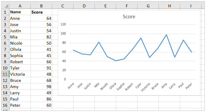
To create a line chart, execute the following steps.
1. Select the range A1:D7.

2. On the Insert tab, in the Charts group, click the Line symbol.

3. Click Line with Markers.

Note: enter a title by clicking on Chart Title. For example, Wildlife Population.
Change Chart Type
You can easily change to a different type of chart at any time.
1. Select the chart.
2. On the Chart Design tab, in the Type group, click Change Chart Type.

3. On the left side, click Column.

4. Click OK.

Switch Row/Column
If you want to display the animals (instead of the months) on the horizontal axis, execute the following steps.
2. On the Chart Design tab, in the Data group, click Switch Row/Column.

Legend Position
To move the legend to the right side of the chart, execute the following steps.
2. Click the + button on the right side of the chart, click the arrow next to Legend and click Right.

Data Labels
You can use data labels to focus your readers' attention on a single data series or data point.
2. Click a green bar to select the Jun data series.
3. Hold down CTRL and use your arrow keys to select the population of Dolphins in June (tiny green bar).
4. Click the + button on the right side of the chart and click the check box next to Data Labels.

1/17 Completed! Learn much more about charts > Go to Next Chapter: Pivot Tables
Learn more, it's easy
- Column Chart
- Scatter Plot
- Data Series
- Combination Chart
- Gauge Chart
- Thermometer Chart
- Gantt Chart
- Pareto Chart
Download Excel File
- charts.xlsx
Next Chapter
- Pivot Tables
Follow Excel Easy
Most Popular
- Formulas and Functions
- Conditional Formatting
- Find Duplicates
- Drop-down List
- Index and Match
Become an Excel Pro
- 300 Examples
Charts • © 2010-2024 Excel is Awesome, we'll show you: Introduction • Basics • Functions • Data Analysis • VBA
Six Sigma & SPC Excel Add-in
- Questions? Contact Us
- 888-468-1537
Key Tools in QI Macros
- Control Charts
- Pareto Charts
- Fishbone Diagrams
Gage R&R Studies
- Data Mining Tools
Statistical Tools
Smart wizards.
Knowledge Base - All Tools
- Free 30-Day Trial
- Powerful SPC Software for Excel
- SPC - Smart Performance Charts
- Who Uses QI Macros?
- What Do Our Customers Say?
- QI Macros SPC Software Reviews
- SPC Software Comparison
- Control Chart
- Histogram with Cp Cpk
- Pareto Chart
- Automated Fishbone Diagram
- Gage R&R MSA
- Statistical Analysis - Hypothesis Testing
- Chart and Stat Wizards
- Lean Six Sigma Excel Templates
- Technical Support - PC
- Technical Support - Mac
- QI Macros FAQs
- Upgrade History
- Submit Enhancement Request
- Data Analysis Services
- Free QI Macros Webinar
- Free QI Macros Video Tutorials
- How to Setup Excel for QI Macros
- Free Healthcare Data Analytics Course
- Free Lean Six Sigma Webinars
- Animated Lean Six Sigma Video Tutorials
- Free Agile Lean Six Sigma Trainer Training
- Free White Belt Training
- Free Yellow Belt Training
- Free Green Belt Training
- QI Macros Resources
- QI Macros Knowledge Base | User Guide
- Excel Tips and Tricks
- Lean Six Sigma Resources
- QI Macros Monthly Newsletter
- Improvement Insights Blog
- Buy QI Macros
- Quantity Discounts and W9
- Hassle Free Guarantee
Home » Training » QI Macros Video Tutorials » Add Text to Excel Chart Point
Want to Add a Note or Description to an Excel Chart Point?
Qi macros makes it easy to add notations or text to a data point..

Why wait? Start creating these charts and diagrams in seconds using QI Macros add-in for Excel.
QI Macros Draws Powerful Smart Charts in Seconds
- Value Stream Maps
Try QI Macros on us!
Or browse all products...
Why Choose QI Macros ?
Affordable - Just $ 369 USD per license - Less with Quantity Discounts - No Recurring Annual Fees - No Charge for Technical Support
Easy to Use - Adds New Tab to Excel's Menu - Creates a Chart in Seconds - PC / Mac: Excel Excel 2013-2021, Office 365
Trusted / Accurate - 100,000 Users in 80 Countries - Save Time vs Writing Formulas - Our Formulas Are Tested
Read What Others Say CNET & Industry Leaders
Verified Customer Reviews
- SPC Software for Excel
- Free 30 Day Trial
- On-line Tech Support
- QI Macros Reviews
- Free QI Macros Training
- Privacy Policy

KnowWare International, Inc. 2696 S. Colorado Blvd., Ste. 555 Denver, CO 80222 USA Toll-Free: 1-888-468-1537 Local: (303) 756-9144
- Testimonials
- Privacy Policy
- Better Data Visualizations
- Book Materials
- Presentation Resources
- Elevate the Debate
- Data Visualization Design Services
- How It Works
- Submit a Visualization
- Infographics Design
- Presentation Slides
- Report Design
- Books About the Brain
- Collaboration Tools
- Color Contrast Tools
- Color Tools
- DataViz Blogs
- DataViz Books
- DataViz Resources
- DataViz Tools
- Design Inspiration
- Design Resources
- Icon Collections
- Image Collections
- PolicyViz Data Visualization Catalog
- Powerpoint and Slide Sharing Tools
- PowerPoint Templates
- Presentation Blogs
- Presentation Books
- Presentation Tools
- Slide Sharing Sites
- Story Books
- Video Editing Tools
- Consulting Services
- Public Workshops
- Virtual Webinars
- Sponsorship Opportunities at PolicyViz
- Terms of Service
- DataViz Design
- Infographics
- Presentations
- Downloads from the Book
- Data Visualization in Excel
- DataViz Catalog
Three Ways to Annotate Your Graphs
Amanda Cox, the editor of the Upshot at the The New York Times , once said that, “The annotation layer is the most important thing we do…otherwise it’s a case of here it is, you go figure it out.”
In my experience, annotating a graph is one of those things that lots of people fail to consider, but it can be a vitally important step to help your reader better understand the context and your argument. It can also be important to simply help your reader understand how to read the graph.
In my view, there are three types of annotation we can include in our data visualizations, moving from simple to more complex: adding labels, creating active titles, and adding detail.
1. Adding Labels
Let’s start with the easiest type of annotation: adding labels. The default in many software tools is to create a data legend and place it below the chart or somewhere to the side, disconnected from the data. This forces your reader to do more work to figure out what each line or bar represents. Instead, a better approach is to directly label your data series. This makes it easier for your reader to connect the data values with its description.
Take a look at this line chart from a paper I wrote on the Disability Insurance program. I included all 50 states plus Washington, DC on the graph and highlighted the seven states of interest. Instead of adding a legend to the top of the graph, I labeled the lines off to the right and color-coded them to match the lines.
This doesn’t have to be complicated or difficult; it just needs to take the reader’s perspective into account. Remember, your audience may not be familiar with the content or the data or simply the presentation of the data, so we want to make it as easy as possible for them to absorb the content. Reducing the amount of time your reader needs to spend understanding what each line or bar represents can help them move to the more important job of understanding the content.
2. Create titles that work as headlines
The next way to annotate your visualizations is to create titles that work as headlines, something I often call “active titles.” Too often, we attach a title to the chart describing the data that are being plotted instead of leading the reader to the point or argument we want to make. Our titles say things like “Figure 1. Support for Targeted and Universal Preschool, 2013.” That could have been the title of the graph from a recent blog post by my Urban colleague Erica Greenberg, but notice how the title of this graph immediately conveys her argument.
A common argument against using more active titles is that the author doesn’t want to seem biased or partisan. I’m not arguing that you use an active title to distort or misrepresent the results, only to put your message in the title. More often than not, when someone argues that they can’t have an active title, I can look in the text next to the graph and see something like, “In Figure 1, you can see that…” Their argument is right next to the graphic, but, like the legend I described above, it’s disconnected from the graph — from the content. Once again, try to integrate your graphs as part of your argument, not as pictures to litter the page.
In Erica’s case, she doesn’t leave it to the reader to figure out what the takeaway point is, nor is she biasing the results by adding commentary in the title; instead, she tells you what you’re supposed to learn from the visual.
3. Adding Detail
Finally, we can provide detail in our graphs to help further convey the argument, highlight specific points, or even explain how to read the graph. In cases where you are visualizing data to help your audience better understand your argument, detailed annotation can help them grasp the context and other key aspects of the graph.
Take this “ Marimekko ” graph about immigration challenges in different countries from former Urban colleague Audrey Singer. The graph shows the relationship between the number of migrants in different countries along the y-axis and migrants as a share of the world’s population along the x-axis. Labeling the bars for the US and Germany, adding an active title and subtitle, and placing a sentence directly in the graph all help the reader understand both how to read the graph and what content they are supposed to absorb from it.
You have certainly seen good examples of annotated graphs when looking at any major newspaper. Sufficient annotation is crucial to helping readers — especially readers who may have less experience with data, statistics, or data visualizations — grasp and understand the content as quickly as possible.
John Burn-Murdoch, an interactive data journalist at the Financial Times once told me that “the annotation layer is where the journalism really comes into visual journalism. Making a graphic is the equivalent to interviewing your source; but it’s then your job to actually pick out…the bits the reader should know about.”
We’re not all journalists, but we all need to find ways to help our readers know what’s important and what we want them to learn.
This post was originally published on the Data@Urban blog on March 17, 2018. Take a look at all the other great stuff we are publishing on Data@Urban and sign-up for the newsletter here .
Share this:
- Click to share on Twitter (Opens in new window)
- Click to share on Facebook (Opens in new window)
- Click to share on LinkedIn (Opens in new window)
- Click to email a link to a friend (Opens in new window)
Thanks for this article. It’s a nice Three Ways to Annotate Your Graphs.
Leave a Reply Cancel reply
Your email address will not be published. Required fields are marked *
Notify me of follow-up comments by email.
Notify me of new posts by email.
Upload image
Guests are limited to images that are no larger than 2MB, and to only jpeg, pjpeg, png file types.
This site uses Akismet to reduce spam. Learn how your comment data is processed .
- Data Accuracy
- Data Journalism
- Data Projects
- DataViz Community
- Presentation Skills
Automatic Excel Chart Annotations
Is there a way to make Excel use a specific column for comments you would like to have automatically (whatever you have entered into a particular cell in the specific column) annotate your chart? For example, I have a chart that shows production of an oil well. The well is shut in for a reason I add to the column. When I create the chart for the production of my well, I want it to automatically add a text box near the value or date when I shut the well in so viewers of the chart know what happened. Is there a way to do this?
About ‘Add, link, edit, or remove titles in a chart’ visit:
Here is a VBA sample how to reference embeded chart and edit title: Sub Chart_Title() Dim oChartObject As ChartObject With ActiveSheet .Range(“F1”).Value = “Chart Title” 'Reference first ChartObject on ActiveSheet Set oChartObject = .ChartObjects(1) End With With oChartObject ‘Assign a name (Constant) to the ChartTitle .Chart.ChartTitle.Text = “My Chart” ‘Link ChartTitle to Excel Cell .Chart.ChartTitle.Text = _ "=’" & ActiveSheet.Name & "’!" & _ ActiveSheet.Range(“F1”).Address End With End Sub
Andrija Vrcan
From: Mike Walker via excel-l [ mailto:[email protected] ] Sent: Thursday, February 18, 2010 1:12 AM To: Andrija Subject: RE: [excel-l] Automatic Excel Chart Annotations
Posted by Mike Walker on Feb 17 at 7:14 PM
Can you manually annotate a chart now? The only text attributes I see for a chart are ChartTitle and AxisTitle (horizontal or vertical). You can change these programmatically to be based on the contents of a cell, but they want to appear as a heading centered above or below the chart, not specific to any data points. Can you just reference the annotation cells underneath your chart - like footnotes? I can draw a textbox on the chart and type into it, but none of that was caught by the macro recorder, so not sure if you could program it to make one either.
Rough code to change Chart or Horizontal Axis Titles: Sub Macro1() ActiveSheet.ChartObjects(“Chart 1”).Activate ActiveChart.ChartTitle.Text = Range(“A2”).Value Range(“A1”).Select End Sub Sub Macro2() ActiveSheet.ChartObjects(“Chart 1”).Activate ActiveChart.Axes(xlCategory).AxisTitle.Select ActiveChart.Axes(xlCategory, xlPrimary).AxisTitle.Text Range(“A3”).Value Range(“A1”).Select End Sub
From: Tonya Nichols via excel-l [ mailto:[email protected] ] Sent: Wednesday, February 17, 2010 6:27 PM To: Mike Walker Subject: [excel-l] Automatic Excel Chart Annotations
Posted by Tonya Nichols (Systems Administrator) on Feb 17 at 6:28 PM
Related Topics
| Topic | Replies | Views | Activity | |
|---|---|---|---|---|
| Programming & Development , | 14 | 171 | May 14, 2009 | |
| Software , | 5 | 230 | March 28, 2013 | |
| Programming & Development , | 9 | 110 | August 7, 2009 | |
| Software , | 13 | 50 | March 5, 2015 | |
| Business , | 2 | 19 | February 8, 2018 |
Search for: Search Button
- How to make a Gantt Chart in Excel
Gantt chart for project management or event scheduling are possible in Excel. Here’s the step-by-step help plus a complete sample worksheet for our subscribers.
Start with a Table
Make a stacked bar chart, add duration series, categories in reverse order, time format / duration, hide unwanted bars with ‘no fill’, sample workbook.
Gantt chart can be widely used in project management for visualizing project schedules. They break down a project or event into tasks or activities as horizontal bars on a timeline. Each bar signifies a task, its length denoting its duration, and its placement indicating its start and end times within the project’s timeline. You can easily see the progress and also when tasks overlap or depend on earlier tasks.
Gantt Charts are possible in Excel though you won’t find them among the supplied charts. We’ll explain how to make a Gantt Chart in Excel then a shortcut for Office Watch subscribers.
We’ll show how to convert a table (above) into a Gantt chart (below) that better shows how the events fit together and how long each lasts.

In the sample spreadsheet we have the “Start Time” and “Duration of the Activity”. The “End Time” is only for our reference and can be calculated from the Start Time and Duration .

Select the Event, Start Time and Minutes and insert a bar chart. Navigate to the “Insert” tab and choose the “Stacked Bar” chart under the 2-D Bar.

As soon as the chart is inserted, Excel will automatically generate horizontal bars representing each task on the timeline.
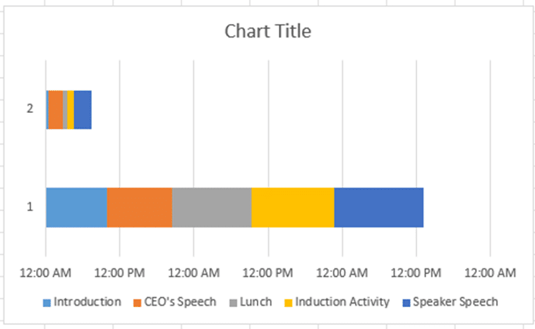
Change the appearance of the chart by right-clicking on the chart and click the “Select data” option.
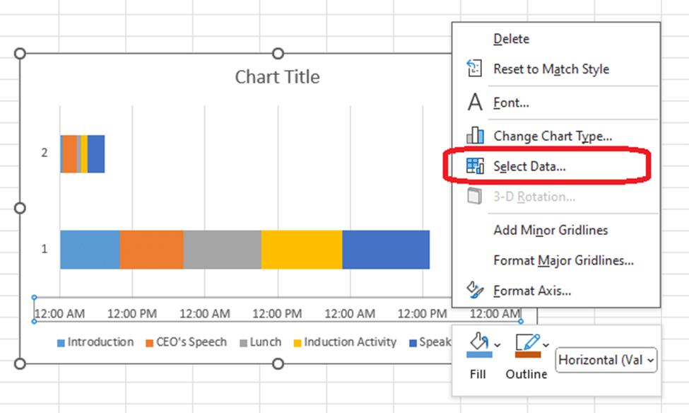
The Select Data pop-up will appear. Click the Switch Row/Column options to interchange the way your data is organized. This can sometimes be necessary to ensure your Gantt chart displays the information correctly.
After clicking this button, you may need to adjust other settings or formatting options to fine-tune your Gantt chart according to your project requirements.
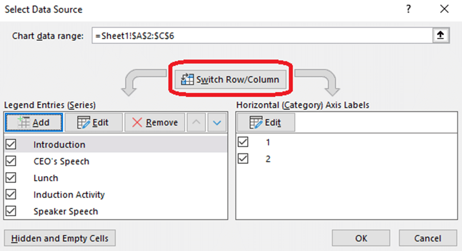
This is how the interim chart should appear:
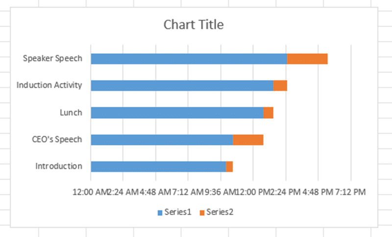
Now you can set up the Duration series, right-click on the Gantt chart, choose Select Data from the menu options, then click “Add” and select the Duration series. This will open the “Select Data Source” dialog box.
In the “Select Data Source” dialog box, click on the “Add” button. This will open the “Edit Series” dialog box.

In the “Edit Series” dialog box, enter the name for your Duration series in the “Series name” field. In the “Series values” field, select the range of cells in your spreadsheet that contain the duration data for your tasks.
Click “OK” to close the “Edit Series” dialog box.
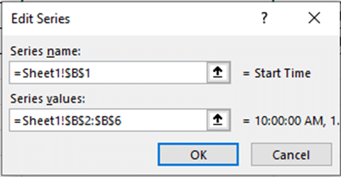
Similarly, In the Edit option, select the Vertical axis values. The vertical axis is the minutes of the event

After all that the chart should look like the one below.
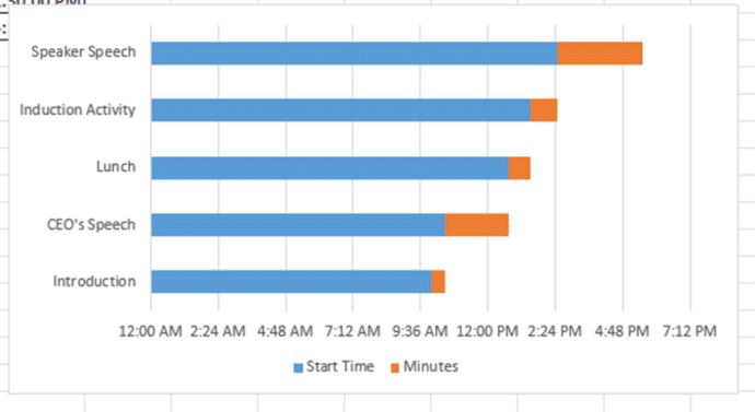
Right-click on the chart, go to Axis Options, and select the “Categories in reverse order” option.
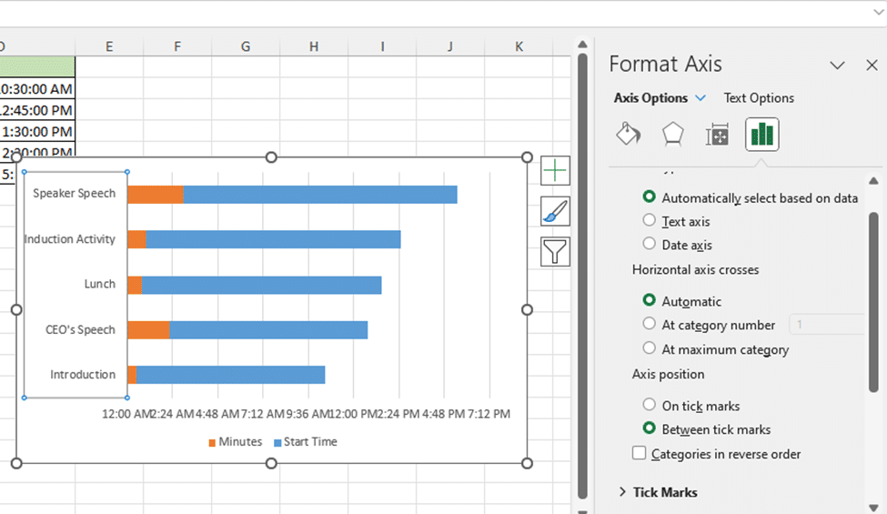
You have the flexibility to select your preferred Time format under the number formatting.

Now Format the Axis options with the following inputs to get the desired Time duration:

The chart now resembles the one below:
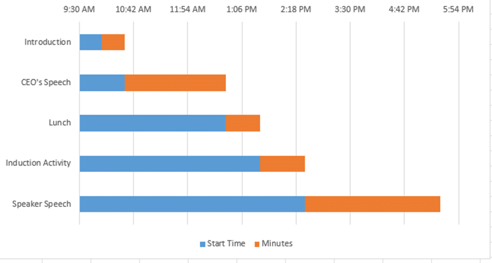
Almost there — the Gantt chart is in place (the orange bars) but with the additional (blue) bars to be hidden.
Select the blue bars in your Gantt chart and format them by setting the “Fill” option to “No fill” to remove any color. Next, remove the gridlines to declutter the chart. Delete the legends to streamline the visualization. Finally, you can add a chart title for clarity and completion if you feel the need.
Now, your Gantt chart is fully prepared and ready to use.
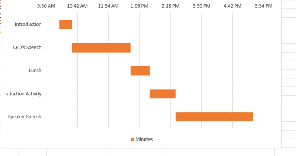
Office Watch subscribers can leap ahead by downloading the complete example worksheet.
It’s a standard Excel .XLS file ( no macros) with a complete working table plus chart. Change the cells highlighted in yellow.
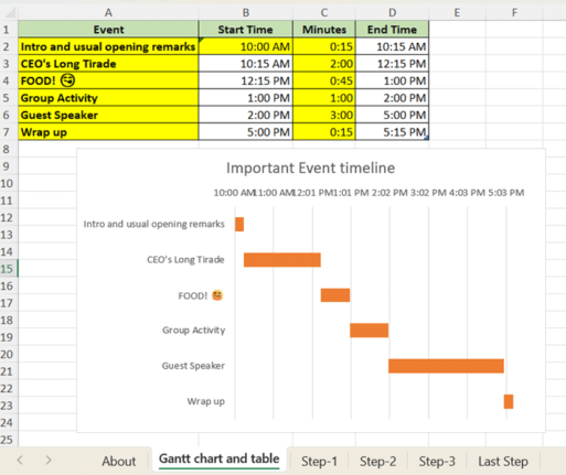
To quickly make a Gantt chart, just change the labels, start time and durations (the yellow cells) and the chart will change.
Add/delete rows to the table and the chart will adjust accordingly.
This download is available EXCLUSIVELY to Office Watch subscribers. The link to this and other special downloads is in each issue of Office Watch or Office for Mere Mortals
Make better Excel Charts by adding graphics or pictures Auto updating your Excel Charts
About this author

Mayurakshi Mohapatra
Office 2021 - all you need to know . Facts & prices for the new Microsoft Office. Do you need it? Office LTSC is the enterprise licence version of Office 2021.
Office 2024 what's known so far plus educated guesses. Microsoft Office upcoming support end date checklist.
Latest from Office Watch
- HUGE news - Excel gets Regular Expression functions
- Surprise! Microsoft recommends Windows 11
- Goggles 🥽 emoji in Word, Excel, PowerPoint and Outlook
- Beware the unexpected when copying an image from Word/Office
- A $125 Billion lesson in why cloud backups are vital
- How Word pastes into your document
- Make monsters and pipes with the Terantopia font
- Avoid the traps when adding Excel info into a Word document
- Circle & Sphere calculations in Excel using Pi 𝜋
- How to list all fonts in a Word document
- Face with rolling eyes 🙄 emoji in Word, Outlook, Office
- Glasses 👓 emoji in Word, Excel, PowerPoint and Outlook
- Calendar extras added to new Outlook
- Changes to PDFs made by Microsoft Office
- It's official - Calibri beats Aptos in font poll
- Vmware Workstation Pro is now free
- A quiet month of security fixes for Microsoft Office
- How Mark of the Web stops bad document infections
- Introducing Reading Coach to enhance Reading Fluency with AI
TechRepublic
Account information.

Share with Your Friends
How to Hide and Handle Zero Values in an Excel Chart
Your email has been sent

Editor’s note: In the video, Brandon Vigliarolo walks you through a couple of ways for suppressing 0 values in Excel charts. For this demo, he uses Microsoft Office 365 . The steps are similar to what Susan Harkins describes in the following tutorial.
A drop to zero in a chart can be abrupt, but sometimes, that’s what you want. On the other hand, there will be times when you won’t want to draw attention to a zero. When you don’t want to display zero values, you have a few choices for how to hide or otherwise manage those zeros.
In this tutorial, I’ll review a few methods for handling zero values that offer quick but limited results with minimal effort. Depending on how much charting you do, you might find more than one of these methods helpful.
Visit Microsoft
Following along
For this demonstration, I’m using Microsoft 365 Desktop on a Windows 11 64-bit system, but you can also use earlier versions of Excel. Excel for the web supports most of these techniques.
SEE: Google Workspace vs. Microsoft 365: A side-by-side analysis w/checklist (TechRepublic Premium)
You can follow along more closely by downloading our demonstration file . If you work through the instructions using our demonstration workbook file, undo each solution before you start the next. You can do this by simply closing the file and reopening it without saving.
Exploring the sample dataset
Figure A shows the data and initial charts that we’ll update throughout this article. The pie and single-line charts reflect the data in column B for Vendor 1. The other two charts have three data series: Vendor 1, Vendor 2 and Vendor 3. The Minimum column returns the minimum value for each month, so April, May and July return zero for the minimum value. This setup simplifies all the examples we’ll be reviewing in this guide.

Right now, the charts display zero values by default in each chart type.
By default, the pie chart, shown in Figure B , charts the zero, but you can’t see it. If you turn on data labels, you will see the zero listed. There are seven slices but eight items in the legend.

Figure C shows the line chart’s default behavior, which drops the one to zero on the X-axis.

Stacked bar chart
Excel plots four stacks for the months without a zero value in the stacked bar chart shown in Figure D . The months with a zero display only two values because the Minimum column also returns zero for those months, so the chart is actually plotting two zeros for each month. Readers might be a bit confused by what they’re seeing.

Multiple-line chart
This multiple-line chart in Figure E is messy; enlarging it doesn’t improve its readability. Although you can’t see all of the lines, they’re there. The values are so close that some lines obscure the others, which is misleading.

Your results may vary, depending on Excel’s default settings and theme colors. Now that you’re familiar with the example data, let’s review a few methods for suppressing the zero values in our example charts. Some will work with limited results and others won’t work at all.
Removing and formatting zero
There’s more than one way to suppress zero values in a chart, but none of them work the same, consistently, for all charts.
Manual removals of zero
To begin with, you might try removing zero values altogether if it’s a literal zero and not the result of a formula. By removing, I mean simply deleting all zero values from the dataset. Unfortunately, this simplest approach doesn’t always work as expected.
The pie chart doesn’t chart the blank cell, but the legend still displays the category label, as you can see in Figure F . Removing the zero values from the dataset changed nothing.

The stacked bar responds interestingly. It doesn’t chart the zero values, as you can see in Figures G, but because the zeros are gone, the MIN() functions in the Minimum column are now all non-zero values and chart accordingly.

Line and multiple-line charts
Neither line chart handles the missing zeros well, but the multiple-line chart is hopeless. The line chart has a gap between the two months, which definitely looks odd ( Figure H) .

The multiple-line chart is deceptive. It appears that the Vendor 1 series is wrong, but if you click it, you will see the markers ( Figure I ). It’s there but obscured by other lines; even doubling its size does nothing to improve its readability.

If you removed zero values in the sheet during this phase, re-enter them before continuing to our next example. Or, close the demonstration file without saving your changes and reopen.
Unchecking worksheet display options
You can also hide zeros by unchecking the worksheet display option called Show A Zero In Cells That Have Zero Value. Here’s how:
1. Click the File tab and choose Options. You might have to click More first.
2. Choose Advanced in the left pane.
3. In the Display Options For This Worksheet section, choose the right sheet from the drop-down menu. (This is a sheet-level property.)
4. Uncheck the Show A Zero In Cells That Have Zero Value option, as shown in Figure J.

5. Click OK.
The zero values still exist — you can see them in the Formula bar. However, Excel won’t display them; thus, this method has no impact. The charts treat the zero values as if they’re still there because they are. Excel for the web doesn’t allow access to this setting.
What we’ve found is that unchecking this setting offers no advantage. I include this step in our tutorial to keep you from wasting your time on this technique yourself.
Setting a custom format
Before you try this next formatting option, reset the Advanced option that you disabled in our previous step, or close the file without saving and reopen it. Keep in mind this next formatting approach has varied results. Here’s how it works:
1. Select the data range B2:D9.
2. Click the Number group’s dialog launcher (Home tab).
3. In the resulting dialog box, choose Custom from the Category list.
4. In the Type control, enter 0,0;;; ( Figure K ) and click OK.

You’ll notice that the results are similar to those seen earlier:
- Pie chart: The pie chart doesn’t chart the zero value, but April is still in the legend.
- Stacked bar chart: The stacked bar chart displays only two stacks for the months with a zero value.
- Line and multiple-line charts: Both line charts include the zero values.
Because these methods are so easy to apply, try deleting the zeros or formatting them first. However, it’s important to recognize that these methods aren’t likely to update all charts the way you want. You might have to find a different solution for each chart!
If you applied this format to the demonstration file, delete it before you continue. Or close the file without saving and then reopen it.
SEE: Here’s how to enter leading zeros in Excel
Charting a filtered dataset
If you have a single data series, you can filter out the zero values and chart the results. Like the methods discussed above, it’s a limited choice because you can only chart one vendor at a time. Additionally, Excel for the web doesn’t support this technique.
Let’s demonstrate. Start by adding a filter to the Vendor 1 column with these steps:
1. Click inside the data range.
2. On the Data tab, click Filter in the Sort & Filter group. If you’re working with a Table object, you can skip this step because the filters are already there.
3. Click Vendor 1’s drop-down and uncheck zero ( Figure L ).

4. Click OK to filter the column, which will filter the entire row. Don’t worry about that, but be sure to remove the filter when you’re done.
Figure M shows the new pie chart.

Figure N shows the new line chart.

Both charts are based on the filtered data in column B. Neither displays the zero value or the category label on the X-axis. However, the line chart has a serious flaw: The line is solid, and April is the same value as March — distributing this chart as-is would be a serious mistake because the data for April is incorrect.
Unfortunately, when you remove the filter, the charts update and display the zero values. On the other hand, if your chart is a one-time task, filtering offers a quick fix for a pie chart.
If you tried this with the demo file, be sure to undo the change or close the file without saving and then reopen it.
Replace zeros with NA()
The most permanent fix for hiding zeros is to replace literal zero values with the NA() function using Excel’s Find and Replace feature. If you update the data regularly, you might even enter NA() for zeros from the get-go, which will eliminate the problem altogether. To do so manually, enter =NA() . However, that’s not always practical, so let’s use Excel’s Replace feature to replace the zero values in the example dataset with the NA() function:
1. Select the dataset. In this case, it’s B2:D9.
2. Click Find & Select in the Editing group on the Home tab and then choose Replace from the dropdown, or press Ctrl + H.
3. Enter 0 in the Find What control.
4. Enter =NA() in the Replace control.
5. If necessary, click Options to display more settings.
6. Check the Match Entire Cell Contents option, as shown in Figure O .

7. Click Replace All, and Excel will replace the zero values.
8. Click OK to dismiss the confirmation message.
9. Click Close.
Figure O above shows the settings and the results. If you don’t select the Match Entire Cell Contents option in step six, Excel will change the values 40, 404 and so on. The formulas in column E display the error value because they’re referencing a cell that displays the error message.
None of the charts display the #N/A error values, but they still display the category label in the axis and the legend. The stacked bar chart displays only two stacks for the months that have a #N/A value, so there’s no difference there. The one curiosity is the multiple-line chart shown in Figure P : The zero values, which are now #N/A error values, are clearly visible.

Suppose you’re working with the results of formulas that might return zero instead of an error value as shown in Figure O . In that case, you can use an IF() function to return the #N/A error using the following syntax:
=IF(formula=0,NA(),formula)
The MIN() function returns the minimum value for each month. The IF() function returns #N/A if the result is zero (Figure Q) :
=IF(MIN(B2:D2)=0,NA(),MIN(B2:D2))

The example’s contrived, but don’t let that bother you. The truth is, you’re unlikely to need this expression because most functions and expressions return the #NA error value if they try to evaluate one.
Choosing from chart settings to chart zero values
Several charts show a gap between one value and another when the zero value is missing. If you’re working with one chart, you can quickly bypass the guesswork by using a chart setting to determine how to chart zero values. Here’s how:
1. Select the chart.
2. Click the contextual Chart Design tab.
3. In the Data group, click Select Data.
4. In the resulting dialog, click the Hidden and Empty Cells button in the bottom-left corner ( Figure R ).

5. Choose one of the options ( Figure S ).

6. Click OK twice to return to the chart.
How do you exclude zero in data labels?
There’s no easy way to remove the zero in data labels. If the chart doesn’t chart it, most of the time it won’t display the value in a data label. After working through all these examples, you can see that the issue comes with no guarantees. You’ll have to explore a bit to find the right settings.
If the chart doesn’t display the zero in the chart or the data label, but does display the series in the legend, you can remove it. Simply select that item in the legend and press Delete. If you accidentally delete all of them, press Ctrl + Z to undo the delete and try again, making sure to select only the one label you want to remove.
There isn’t an easy one-size-fits-all solution for the problem of zeroless charts. If you’re displaying zeros for reporting purposes, but you don’t want to see them in charts and you’re charting often, consider maintaining two datasets: One for reporting and one for charting. This is the best alternative to toggling back and forth with one dataset.
The real problem is the story the data tells. Zero is a valid value and Excel treats it as such.
Read next: Explore some of the best free alternatives to Microsoft Excel .
Subscribe to the Developer Insider Newsletter
From the hottest programming languages to commentary on the Linux OS, get the developer and open source news and tips you need to know. Delivered Tuesdays and Thursdays
- 9 best data science tools and software of 2023
- 8 Best ETL Tools and Software of 2023
- Hiring kit: GDPR data protection compliance officer
- Big data: More must-read coverage

Create a TechRepublic Account
Get the web's best business technology news, tutorials, reviews, trends, and analysis—in your inbox. Let's start with the basics.
* - indicates required fields
Sign in to TechRepublic
Lost your password? Request a new password
Reset Password
Please enter your email adress. You will receive an email message with instructions on how to reset your password.
Check your email for a password reset link. If you didn't receive an email don't forgot to check your spam folder, otherwise contact support .
Welcome. Tell us a little bit about you.
This will help us provide you with customized content.
Want to receive more TechRepublic news?
You're all set.
Thanks for signing up! Keep an eye out for a confirmation email from our team. To ensure any newsletters you subscribed to hit your inbox, make sure to add [email protected] to your contacts list.
- Application management

- Alexander S. Gillis, Technical Writer and Editor
What is Excel?
Excel is a spreadsheet program from Microsoft and a component of its Office product group for business applications. Microsoft Excel enables users to format, organize and calculate data in a spreadsheet.
By organizing data using software like Excel, data analysts and other users can make information easier to view as data is added or changed. Excel contains a large number of boxes called cells that are ordered in rows and columns. Data is placed in these cells.
Excel is a part of the Microsoft Office and Office 365 suites and is compatible with other applications in the Office suite. The spreadsheet software is available for Windows, macOS, Android and iOS platforms.
Common Excel use cases
Excel is most commonly used in business settings. For example, it is used in business analysis, human resource management , operations management and performance reporting. Excel uses a large collection of cells formatted to organize and manipulate data and solve mathematical functions. Users can arrange data in the spreadsheet using graphing tools, pivot tables and formulas. The spreadsheet application also has a macro programming language called Visual Basic for Applications.
Organizations use Microsoft Excel for the following:
- collection and verification of business data;
- business analysis;
- data entry and storage;
- data analysis;
- performance reporting;
- strategic analysis;
- accounting and budgeting;
- administrative and managerial management;
- account management;
- project management ; and
- office administration.
Excel terminology and components
Excel has its own terminology for its components, which new users may not immediately find understandable. Some of these terms and components include the following:
- Cell. A user enters data into a cell, which is the intersection of a column and row.
- Cell reference. This is the set of coordinates where a cell is located. Rows are horizontal and numbered whereas columns are vertical and assigned a letter.
- Active cell. This is the currently selected cell, outlined by a green box.
- Workbook. This is an Excel file that contains one or more worksheets.
- Worksheet. These are the different documents nested within a Workbook.
- Worksheet tab. These are the tabs at the bottom left of the spreadsheet.
- Column and row headings. These are the numbered and lettered cells located just outside of the columns and rows. Selecting a header highlights the entire row or column.
- Formula. Formulas are mathematical equations, cell references or functions that can be placed inside a cell to produce a value. Formulas must start with an equal "=" sign.
- Formula bar. This is the long input bar that is used to enter values or formulas in cells. It is located at the top of the worksheet, next to the "fx" label.
- Address bar. This bar located to the left of the formula bar shows the number and letter coordinates of an active cell.
- Filter. These are rules a user can employ to select what rows in a worksheet to display. This option is located on the top right of the home bar under "Sort & Filter." An auto filter option can be selected to show rows that match specific values.
- AutoFill. This feature enables users to copy data to more than one cell automatically. With two or more cells in a series, a user can select both cells and drag the bottom right corner down to autofill the rest of the cells.
- AutoSum. This feature enables users to add multiple values. Users can select the cells they want to add and press the Alt and Equal keys. There is also a button to enable this feature on the top right of the home page, above "Fill" and to the left of "Sort & Filter."
- PivotTable. This data summarization tool sorts and calculates data automatically. This is located under the insert tab on the far left.
- PivotChart. This chart acts as a visual aid to the PivotTable, providing graph representations of the data. It is located under the middle of the insert page, next to maps.
- Source data. This is the information that is used to create a PivotTable.

Advanced Excel capabilities
More advanced tools in Excel include the following:
- TREND function. This tool is used to calculate linear trend lines through a set of Y or X values. It can be used for time series trend analysis or projecting future trends. Trendlines can be used on charts.
- VLOOKUP. The Vertical Lookup, or VLOOKUP function, can be used to search for values in a larger data set and pull that data into a new table. VLOOKUP is a cell input command that looks like =VLOOKUP(). The parentheses include the data the user wants to look up, where to look for it, the column number with the value to return; or optionally, the user can specify an Approximate or Exact match indicated by True or False.
- Table Array. This is a combination of two or more tables with data and values linked and related to one another. This is part of VLOOKUP.
- Col_index_num. Another value when creating a table array that specifies the column from where data is being pulled.
- Range_lookup. This value in VLOOKUP provides information closest to what a user wants to find when nothing matches other variables. This is represented by a true or false label. False gives the exact value a user is looking for and True gives results from a variable data range.
- MAX and MIN functions. These functions provide the maximum and minimum values from selected data sets. MAX is used to find the maximum value in a function tab and MIN is used to find the minimum value.
- AND function. This function has more than one criteria set when searching variables. If a variable matches the criteria, the value will be returned as true; if not, it will be returned as false. The input for the function should look like this: =AND (logical1, [logical2], ...).
Additional functions for use in Excel include subtract, multiply, divide, count, median, concatenate and other logical functions similar to AND, such as OR.
Excel and XLS files
An XLS file is a spreadsheet file that can be created by Excel or other spreadsheet programs. The file type represents an Excel Binary File format. An XLS file stores data as binary streams -- a compound file. Streams and substreams in the file contain information about the content and structure of an Excel workbook.
Versions of Excel after Excel 2007 use XLSX files by default, since it is a more open and structured format. Later versions of Excel still support the creation and reading of XLS files, however. Workbook data can also be exported in formats including PDF, TXT, Hypertext markup language, XPS and XLSX.
Macro-enabled Excel files use the XLSM file extension. In this case, macros are sets of instructions that automate Excel processes. XLSM files are similar to XLM files but are based on the Open XML format found in later Microsoft Office software.
Excel competitors
Even though Excel might be one of the most recognizable spreadsheet programs, other vendors offer competing products. Examples include the following:
- Google Sheets . Google Sheets is a free competitor to Excel, with similar layouts and features. Users with a Gmail account can access Google Sheets. Google Sheets are saved in the cloud, meaning users can access their spreadsheets from anywhere and on numerous devices. Multiple users can also collaborate on the same spreadsheet.
- Numbers. Apple's spreadsheet program comes free with every Mac and provides prebuilt templates, charts and graphs. Numbers excels at graphics and charts, but it does not handle large data sets as well as Microsoft Excel. Numbers is also exclusive for Apple's devices. But it does enable users to save spreadsheets as Excel files, so a Windows user can still open a Numbers spreadsheet in Excel.
- Apache OpenOffice Calc. This free open source spreadsheet software features multiple user collaboration; natural language formulas that enable users to create formulas using words; DataPilot, which pulls data from corporate databases; and style and formatting features that enable different cell formatting options. The software uses a different macro programming language than Excel and has fewer chart options. OpenOffice Calc works on Windows and macOS platforms. OpenOffice Calc also uses the Open Document Format as its default, with only limited support for Microsoft's XLSX format.

History and future of Excel
Microsoft released Excel in 1985 under the name Microsoft Multiplan. Microsoft's spreadsheet program competed with similar products at the time, including Lotus 1-2-3 from the Lotus Development Corp. Although Lotus 1-2-3 was reportedly the first spreadsheet to introduce cell names and macros, Multiplan used a graphical user interface and enabled users to point and click using a mouse. Multiplan made it easier to manipulate, process and view spreadsheet data.
Initially, Multiplan lost popularity on Microsoft Disk Operating System ( MS-DOS ) systems when competing with Lotus 1-2-3. Two years after its initial release, in 1987, Microsoft introduced Excel version 2.0. By 1988, this new version, now on Windows platforms, began to outsell Lotus 1-2-3 and other similar spreadsheet programs.
In 1990, Microsoft released version 3 of Excel, with features such as toolbars, 3D charts, and drawing and outlining capabilities. Version 4 came along two years later and added the auto-fill function. In 1993, version 5 of Excel was released. This version included Visual Basic for Applications macros, which enabled regular tasks to be automated.
One of the next big updates to Excel was version 12, which was released in 2007. This update used a new Ribbon menu system. Improved functions included a SmartArt set of diagrams, better management of named variables and more flexibility for formatting graphs. Excel moved to using the more structured and open XLSX files as well. Version 15 released in 2013 included new tools such as Power View, Power Pivot and Flash Fill. This version also improved multithreading capabilities.
The current version of Excel, version 16, was released in 2019. Since its conception, Microsoft Excel has become one of the most widely used business applications and is often paired with other Microsoft apps such as Word, Outlook and PowerPoint. Although Microsoft no longer updates Excel as different versions, it rolls out new features and updates automatically over time.
Microsoft Excel is arguably one of the most popular spreadsheet applications and has long since played a role in businesses. However, with the popularity of other current spreadsheet software, Excel now has increased competition. The website askwonder.com claims that the collection of apps in Google Suite, which includes Google Sheets, is used by 2 billion users every month, whereas Microsoft Excel has an estimated 750 million to 1.2 billion monthly global users. Google and Microsoft do not publish monthly usage for either spreadsheet program, so it is difficult to estimate values.
Learn more about the different benefits of using Excel for HR in this article.
Continue Reading About Excel
- Google announces G Suite overhaul with Google Workspace
- How to find the top 3 values using the Excel LARGE function
- Excel is the hammer for too many businesses' nails
- Are there viable spreadsheet app alternatives to Microsoft Excel?
- What to keep in mind when creating data visualization in Excel
Related Terms
Dig deeper on application management.

Reviewing the features of Copilot for Microsoft 365

Apache OpenOffice

How to use the Excel LARGE function, with examples
With the acquisition of Cameyo, Google puts ChromeOS into consideration in enterprises alongside thin clients, repurposed PCs or ...
VMware EUC users waiting to see where the products would land after Broadcom's divestiture now have some answers.
Government organizations should turn to the variety of dedicated services that Microsoft offers to deliver familiar productivity ...
Admins need all the help they can get, and this Microsoft utility shows IT how to correct security issues and optimize ...
Learn how to simplify user provisioning in the cloud collaboration platform with faster results by seeing examples of scripts ...
Automation is a good way for admins to handle all the tasks associated with removing a user from the organization's tenant in ...
'ZDNET Recommends': What exactly does it mean?
ZDNET's recommendations are based on many hours of testing, research, and comparison shopping. We gather data from the best available sources, including vendor and retailer listings as well as other relevant and independent reviews sites. And we pore over customer reviews to find out what matters to real people who already own and use the products and services we’re assessing.
When you click through from our site to a retailer and buy a product or service, we may earn affiliate commissions. This helps support our work, but does not affect what we cover or how, and it does not affect the price you pay. Neither ZDNET nor the author are compensated for these independent reviews. Indeed, we follow strict guidelines that ensure our editorial content is never influenced by advertisers.
ZDNET's editorial team writes on behalf of you, our reader. Our goal is to deliver the most accurate information and the most knowledgeable advice possible in order to help you make smarter buying decisions on tech gear and a wide array of products and services. Our editors thoroughly review and fact-check every article to ensure that our content meets the highest standards. If we have made an error or published misleading information, we will correct or clarify the article. If you see inaccuracies in our content, please report the mistake via this form .
How to use ChatGPT to make charts and tables with Advanced Data Analysis

Know what floats my boat? Charts and graphs.
Give me a cool chart to dig into and I'm unreasonably happy. I love watching the news on election nights, not for the vote count, but for all the great charts. I switch between channels all evening to see every possible way that each network finds to present numerical data.
Is that weird? I don't think so.
Also: The moment I realized ChatGPT Plus was a game-changer for my business
As it turns out, ChatGPT does a great job making charts and tables. And given that this ubiquitous generative AI chatbot can synthesize a ton of information into something chart-worthy, what ChatGPT gives up in pretty presentation it more than makes up for in informational value.
It should come as no surprise to anybody that AI chatbots' feature sets are changing constantly. As of the time of this update (end of May, 2024), OpenAI has just come out with a Mac application and has release its GPT-4o LLM, which is available for both free and paying customers. The GPT-4o version that comes for the added-price Plus version is supposed to have interactive chart features and the ability to interact with the engine longer per session.
But, not so much. My free account doesn't offer GPT-4o at all yet. It hasn't rolled out to all free accounts yet. And while paid ChatGPT Plus plan does provide the interactive charts feature in Chrome and Safari, it doesn't in the Mac app.
Also: ChatGPT vs. ChatGPT Plus: Is a paid subscription still worth it?
This article was last updated when the Advanced Data Analysis features (which included charts) were only available to Plus customers. Even though some of those features are supposed to be available to free customers, since my free account doesn't have them yet, I'm going to present the rest of this article as if the charting features are only available to Plus customers. If you're a free customer and you have GPT-4o, feel free to try some of the prompts. Those features may work for you, and undoubtely will as we move forward in time.
Advanced Data Analysis produces relatively ugly charts. But it rocks. First, let's discuss where ChatGPT gets its data, then we'll make some tables.
How to use ChatGPT to make charts and tables
1. understand the different versions of chatgpt.
Earlier, we talked about which charting tools are available in which versions of ChatGPT. But there's more to it than simply charting tools. If you want to use ChatGPT productively, you need to understand what the various editions can do.
ChatGPT free version: This version has historically used the GPT-3.5 large language model (LLM), which isn't quite as capable as the GPT-4 version . As of May 2024, the GPT-4o LLM is also available to some free users and rolling out over time.
ChatGPT Plus: ChatGPT Plus is OpenAI's commercial, fully powered version of ChatGPT. Right now, ChatGPT Plus provides three major selection options per session: GPT-3.5, GPT-4, and GPT-4o. It used to offer plugins, but they've been replaced by custom GPTs .
The GPT-4 and GPT-4o versions now include DALL-E 3, Bing Web access, and Advanced Data Analysis. Some users have reported some difficulty with using Bing for web access. Most of what we will be doing is using the Advanced Data Analysis component. Even without Bing web access, GPT-4 and 4o report that training data now includes information up to December 2023.
Also: What does GPT stand for? Understanding GPT 3.5, GPT 4, GPT-4o, and more
For much of this article, we will be using the Advanced Data Analysis component of the GPT-4 option. This tool will import data tables in a wide range of file formats. While it doesn't specify a size limit for imported data, it can handle fairly large files, but will break if the files exceed some undefined level of complexity.
As ChatGPT Plus changes, and it will, we will update you with more information. For now, let's just look at making some cool charts.
ChatGPT Enterprise: Advanced Data Analytics and plugins are also available in the enterprise version . You can upload files to Enterprise, and they will remain confidential. Enterprise is also supposed to allow for bigger files and bigger responses. Pricing has not been specified.
2. Create a basic table
Let's start with an example. For the following demonstration, we'll be working with the top five cities in terms of population.
List the top five cities in the world by population. Include country.
I asked this question to ChatGPT's free version and here's what I got back:
Turning that data into a table is simple. Just tell ChatGPT you want a table:
Make a table of the top five cities in the world by population. Include country.
3. Manipulate the table
You can manipulate and customize a table by giving ChatGPT more detailed instructions. Again, using the free version, we'll add a population count field. Of course, that data is out of date, but it's presented anyway:
Make a table of the top five cities in the world by population. Include country and a population field
You can also specify certain details for the table, like field order and units. Here, I'm moving the country first and compressing the population numbers.
Make a table of the top five cities in the world by population. Include country and a population field. Display the fields in the order of rank, country, city, population. Display population in millions (with one decimal point), so 37,833,000 would display as 37.8M.
Note that I gave the AI an example of how I wanted the numbers to display.
That's about as far as the free version will take us. From now on, we're switching to the $20/month ChatGPT Plus version .
4. Create a bar chart
ChatGPT Plus with Advanced Data Analytics enabled can make line charts, bar charts, histograms, pie charts, scatter plots, heatmaps, box plots, area charts, bubble charts, Gantt charts, Pareto charts, network diagrams, Sankey diagrams, choropleth maps, radar charts, word clouds, treemaps, and 3D charts.
In this example, we're just going to make a simple bar chart.
Make a bar chart of the top five cities in the world by population
Chatty little tool, isn't it?
The eagle-eyed among you may have noticed the discrepancy in populations between the previous table shown and the results here. Notice that the table has a green icon and this graph has a purple icon. We've jumped from GPT-3.5 (the free version of ChatGPT) to GPT-4 (in ChatGPT Plus). It's interesting that the differing LLMs have slightly different data. This difference is all part of why it pays to be careful when using AIs, so double-check your work. In our case, we're just demonstrating charts, but this is a tangible example of where confidently presented data can be wrong or inconsistent.
5. Upload data
One of Advanced Data Analytics' superpowers is the ability to upload a dataset. For our example, I downloaded the Popular Baby Names dataset from Data.gov . This is a comma-separated file of New York City baby names from 2011-2014. Even though it's a decade out of date, it's fun to play with.
The dataset I chose for this article is readily available from a government site, so you can replicate this experiment on your own. There are a ton of great datasets available on Data.gov , but I found that many are far too large for ChatGPT to use.
Also: How to use ChatGPT to create an app
Once I downloaded this one, I realized it also included information on ethnicity, so we can run a number of different charts from the same dataset.
Click the little upload button and then tell it the data file you want to import.
I asked it to show me the first five lines of the file so I'd know more about the file's format.
6. Create a pie chart (and change colors)
I was curious about how the dataset distributed gender names. Here's my first prompt:
Create a pie chart showing gender as a percentage of the overall dataset
And here's the result:
Unfortunately, the dark shade of green makes the numbers difficult to read. Fortunately, you can instruct Advanced Data Analytics to use different colors. I was careful to choose colors that did not reinforce gender stereotypes.
Create a pie chart showing gender as a percentage of the overall dataset. Use light green for male and medium yellow for female.
7. Normalize data for accuracy
As we saw earlier, the data collected includes ethnicity. Here's how to see the distribution of the various ethnicities New York recorded in the early 2010s:
Show the distribution of ethnicity in the dataset using a pie chart. Use only light colors.
And here's the result. Notice anything?
Apparently, New York didn't properly normalize its data. It used "WHITE NON HISPANIC" and "WHITE NON HISP" together, "BLACK NON HISPANIC" and "BLACK NON HISP" together, and "ASIAN AND PACIFIC ISLANDER" and "ASIAN AND PACI" together. This resulted in inaccurate representations of the data.
One benefit of ChatGPT is it remembers instructions throughout a session. So I was able to give it this instruction:
For all the following requests, group "WHITE NON HISPANIC" and "WHITE NON HISP" together. Group "BLACK NON HISPANIC" and "BLACK NON HISP" together. Group "ASIAN AND PACIFIC ISLANDER" and "ASIAN AND PACI". Use the longer of the two ethnicity names when displaying ethnicity.
And it replied:
Let's try the chart again, using the same prompt.
That's better:
You need to be diligent when looking at results. For example, in a request for top baby names, the AI separated out "Madison" and "MADISON" as two different names:
For all the following requests, baby names should be case insensitive.
8. Export your graphics
Let's wrap up with a complex chart from one prompt. Here's our prompt:
For each ethnicity, present two pie charts, one for each gender. Each pie chart should list the top five baby names for that gender and that ethnicity. Use only light colors.
As it turns out, the chart generated text that was too small to read. So, to get a more useful chart, we can export it back out. I'm going to specify both file format and file width:
Export this chart as a 3000 pixel wide JPG file.
Notice that Sofia and Sophia are very popular, but are shown as two different names. But that's what makes charts so fascinating.
How much does it cost to use Advanced Data Analytics?
Advanced Data Analytics comes with ChatGPT Plus. Some of its features are available in GPT-4o for the free version of ChatGPT. ChatGPT Plus is $20/month. Advanced Data Analytics also is included with the Enterprise edition, but pricing for that hasn't been released yet.
Is the data uploaded to ChatGPT for charting kept private or is there a risk of data exposure?
Assume that there's always a privacy risk.
I asked this question to ChatGPT and this is what it told me:
Data privacy is a priority for ChatGPT. Uploaded data is used solely for the purpose of the user's current session and is not stored long-term or used for any other purposes. However, for highly sensitive data, users should always exercise caution and consider using the Enterprise version of ChatGPT, which offers enhanced data confidentiality.
Also: Generative AI brings new risks to everyone. Here's how you can stay safe
My recommendation: Don't trust ChatGPT or any generative AI tool. The Enterprise version is supposed to have more privacy controls, but I would recommend you only upload data that you won't mind finding its way to public visibility.
Can ChatGPT's Advanced Data Analysis handle real-time data or is it more suited for static datasets?
It's possible, but there are some practical limitations. First, the Plus account will throttle the number of requests you can make in a given period of time. Second, you have to upload each file individually. There is the possibility you could use a licensed ChatGPT API to do real-time analytics. But for the chatbot itself, you're looking at parsing data at rest.
You can follow my day-to-day project updates on social media. Be sure to subscribe to my weekly update newsletter on Substack , and follow me on Twitter at @DavidGewirtz , on Facebook at Facebook.com/DavidGewirtz , on Instagram at Instagram.com/DavidGewirtz , and on YouTube at YouTube.com/DavidGewirtzTV .
Artificial Intelligence
The best satellite phones you can buy: expert tested, this power station has an irreplaceable emergency feature (and is $400 off right now), the best web hosting services: expert tested.
Help | Advanced Search
Computer Science > Machine Learning
Title: fastgas: fast graph-based annotation selection for in-context learning.
Abstract: In-context learning (ICL) empowers large language models (LLMs) to tackle new tasks by using a series of training instances as prompts. Since generating the prompts needs to sample from a vast pool of instances and annotate them (e.g., add labels in classification task), existing methods have proposed to select a subset of unlabeled examples for annotation, thus enhancing the quality of prompts and concurrently mitigating annotation costs. However, these methods often require a long time to select instances due to their complexity, hindering their practical viability. To address this limitation, we propose a graph-based selection method, FastGAS, designed to efficiently identify high-quality instances while minimizing computational overhead. Initially, we construct a data similarity graph based on instance similarities. Subsequently, employing a graph partitioning algorithm, we partition the graph into pieces. Within each piece (i.e., subgraph), we adopt a greedy approach to pick the most representative nodes. By aggregating nodes from diverse pieces and annotating the corresponding instances, we identify a set of diverse and representative instances for ICL. Compared to prior approaches, our method not only exhibits superior performance on different tasks but also significantly reduces selection time. In addition, we demonstrate the efficacy of our approach in LLMs of larger sizes.
| Subjects: | Machine Learning (cs.LG); Artificial Intelligence (cs.AI) |
| Cite as: | [cs.LG] |
| (or [cs.LG] for this version) | |
| Focus to learn more arXiv-issued DOI via DataCite |
Submission history
Access paper:.
- HTML (experimental)
- Other Formats
References & Citations
- Google Scholar
- Semantic Scholar
BibTeX formatted citation
Bibliographic and Citation Tools
Code, data and media associated with this article, recommenders and search tools.
- Institution
arXivLabs: experimental projects with community collaborators
arXivLabs is a framework that allows collaborators to develop and share new arXiv features directly on our website.
Both individuals and organizations that work with arXivLabs have embraced and accepted our values of openness, community, excellence, and user data privacy. arXiv is committed to these values and only works with partners that adhere to them.
Have an idea for a project that will add value for arXiv's community? Learn more about arXivLabs .
IMAGES
VIDEO
COMMENTS
Annotating a graph in Excel is a useful feature that allows you to add text, shapes, arrows, and data labels to your graph to emphasize important points or trends. Here's a step-by-step guide on how to annotate a graph in Excel. How to add text annotations to a graph.
How to add a text box to a chart in Word, Excel, PowerPoint, and Outlook.
How to Annotate Excel Charts. Part of the series: Basics of Microsoft Excel. Annotating Excel charts is a great way to add additional information to very spe...
Want to annotate your charts added in Microsoft Excel? Now Microsoft Excel empowers you to annotate charts with just few single clicks. So watch this video t...
Subscribe Now:http://www.youtube.com/subscription_center?add_user=ehowtechWatch More:http://www.youtube.com/ehowtechAnnotating a graph in Excel is a great wa...
On a chart, click the title, label, or text box that you want to link to a worksheet cell, or do the following to select it from a list of chart elements. Click a chart. This displays the Chart Tools tabs. Note: The names of the tabs within Chart Tools differs depending on the version of Excel you are using.
Excel 2013 also lets you put numbers from your spreadsheet into your data labels - that is, numbers that are not directly associated with the data point. Here is a quick example. Let's say that I want to add a further annotation about the temperature on Wednesday and I want to include a data value with that annotation.
To quickly identify a data series in a chart, you can add data labels to the data points of the chart. By default, the data labels are linked to values on the worksheet, and they update automatically when changes are made to these values.
Purpose — to add a data label to just ONE POINT on a chart in Excel. There are situations where you want to annotate a chart line or bar with just one data label, rather than having all the data points on the line or bars labelled.
The following chart uses a link to a cell value to show the total cells in the chart title. However, you are not limited to these built-in labels. You can include captions in Excel graphs by adding text boxes.
Note: If you are using Excel 2010, please click Layout > Text Box under Chart Tools. 2. Draw a text box in the chart area as below screenshot shown, and type the note content as you need in the text box. 3. Format the note font as you need with features in the Font group on the Home tab, such as change font size, add font color, bold, etc.
The tutorial shows how to create and customize graphs in Excel: add a chart title, change the way that axes are displayed, format the chart legend, add data labels, and more.
On an Excel time graph, how do I add an annotation on a single data point? At the place where the orange line becomes flat below, the temperature of a..
Microsoft Excel's quick-format chart and graph features offer a way to instantly convert your data-filled cells into a visual representation such as a pie chart or bar graph.
Annotate and label charts. The Annotate Chart function provides a simple way to add comments and color to individual data points in your chart. For example, you can easily highlight specific points in a scatter plot, or you could add asterisks ("stars", "*") to a bar graph with a mouse click to denote statistical significance.
Labelling Events in Excel Charts helps explain blips, patterns and trends in data. It's useful for line and column charts that span time.
Here's how to make a chart, commonly referred to as a graph, in Microsoft Excel. How to Create a Graph or Chart in Excel Excel offers many types of graphs from funnel charts to bar graphs to waterfall charts. You can review recommended charts for your data selection or choose a specific type.
See how to quickly identify, highlight and label a specific data point in a scatter chart in Excel, and how to define its position on the x and y axes.
A simple chart in Excel can say more than a sheet full of numbers. As you'll see, creating charts is very easy.
How to Annotate a Graph in Excel. Part of the series: Office Software Help. Annotating a graph in Excel is a great way to provide useful context to the infor...
Want to add a note or text to an Excel chart point? This video shows how easy QI Macros makes it to add notations and descriptions to data points. No cc req to download 30-day trial.
2. Create titles that work as headlines. The next way to annotate your visualizations is to create titles that work as headlines, something I often call "active titles.". Too often, we attach a title to the chart describing the data that are being plotted instead of leading the reader to the point or argument we want to make.
Is there a way to make Excel use a specific column for comments you would like to have automatically (whatever you have entered into a particular cell in the specific column) annotate your chart? For example, I have a chart that shows production of an oil well. The well is shut in for a reason I add to the column. When I create the chart for the production of my well, I want it to ...
Gantt Charts are possible in Excel though you won't find them among the supplied charts. We'll explain how to make a Gantt Chart in Excel then a shortcut for Office Watch subscribers. We'll show how to convert a table (above) into a Gantt chart (below) that better shows how the events fit together and how long each lasts.
Here are a few techniques to hide and manage zeros in your workbook to avoid confusion caused by unintended results from missed zeroes.
Budgeting, chart creation, data analytics and more - all at your fingertips. The Excel spreadsheet and budgeting app lets you create, view, edit and share files, charts and data. Excel's built-in file editor lets you manage your finances with on-the-go budget and expense tracking integration. We make it easy to review and analyze data, edit ...
The Excel spreadsheet app lets you create, view, edit, and share your files with others quickly and easily. Create spreadsheets, data analyses, charts, budgets and more while you view and edit workbooks attached to email messages. ... • Chart maker to annotate, edit and insert charts that bring your data to life. • Data analysis features ...
Excel is a spreadsheet program from Microsoft, a component of its Office product group for business applications. In common with similar products, such as Lotus 1-2-3 and Corel's QuattroPro, Excel is an automated version of the paper-based spreadsheet that makes it easier to manipulate, process, and view the data. Although Lotus 1-2-3 was ...
ChatGPT has some great chart-making tools. From histograms and heatmaps to word clouds and network diagrams, here's how to take full advantage of this powerful capability.
In-context learning (ICL) empowers large language models (LLMs) to tackle new tasks by using a series of training instances as prompts. Since generating the prompts needs to sample from a vast pool of instances and annotate them (e.g., add labels in classification task), existing methods have proposed to select a subset of unlabeled examples for annotation, thus enhancing the quality of ...