Have a language expert improve your writing
Run a free plagiarism check in 10 minutes, generate accurate citations for free.
- Knowledge Base
Methodology
- What Is a Case-Control Study? | Definition & Examples

What Is a Case-Control Study? | Definition & Examples
Published on February 4, 2023 by Tegan George . Revised on June 22, 2023.
A case-control study is an experimental design that compares a group of participants possessing a condition of interest to a very similar group lacking that condition. Here, the participants possessing the attribute of study, such as a disease, are called the “case,” and those without it are the “control.”
It’s important to remember that the case group is chosen because they already possess the attribute of interest. The point of the control group is to facilitate investigation, e.g., studying whether the case group systematically exhibits that attribute more than the control group does.
Table of contents
When to use a case-control study, examples of case-control studies, advantages and disadvantages of case-control studies, other interesting articles, frequently asked questions.
Case-control studies are a type of observational study often used in fields like medical research, environmental health, or epidemiology. While most observational studies are qualitative in nature, case-control studies can also be quantitative , and they often are in healthcare settings. Case-control studies can be used for both exploratory and explanatory research , and they are a good choice for studying research topics like disease exposure and health outcomes.
A case-control study may be a good fit for your research if it meets the following criteria.
- Data on exposure (e.g., to a chemical or a pesticide) are difficult to obtain or expensive.
- The disease associated with the exposure you’re studying has a long incubation period or is rare or under-studied (e.g., AIDS in the early 1980s).
- The population you are studying is difficult to contact for follow-up questions (e.g., asylum seekers).
Retrospective cohort studies use existing secondary research data, such as medical records or databases, to identify a group of people with a common exposure or risk factor and to observe their outcomes over time. Case-control studies conduct primary research , comparing a group of participants possessing a condition of interest to a very similar group lacking that condition in real time.
Receive feedback on language, structure, and formatting
Professional editors proofread and edit your paper by focusing on:
- Academic style
- Vague sentences
- Style consistency
See an example

Case-control studies are common in fields like epidemiology, healthcare, and psychology.
You would then collect data on your participants’ exposure to contaminated drinking water, focusing on variables such as the source of said water and the duration of exposure, for both groups. You could then compare the two to determine if there is a relationship between drinking water contamination and the risk of developing a gastrointestinal illness. Example: Healthcare case-control study You are interested in the relationship between the dietary intake of a particular vitamin (e.g., vitamin D) and the risk of developing osteoporosis later in life. Here, the case group would be individuals who have been diagnosed with osteoporosis, while the control group would be individuals without osteoporosis.
You would then collect information on dietary intake of vitamin D for both the cases and controls and compare the two groups to determine if there is a relationship between vitamin D intake and the risk of developing osteoporosis. Example: Psychology case-control study You are studying the relationship between early-childhood stress and the likelihood of later developing post-traumatic stress disorder (PTSD). Here, the case group would be individuals who have been diagnosed with PTSD, while the control group would be individuals without PTSD.
Case-control studies are a solid research method choice, but they come with distinct advantages and disadvantages.
Advantages of case-control studies
- Case-control studies are a great choice if you have any ethical considerations about your participants that could preclude you from using a traditional experimental design .
- Case-control studies are time efficient and fairly inexpensive to conduct because they require fewer subjects than other research methods .
- If there were multiple exposures leading to a single outcome, case-control studies can incorporate that. As such, they truly shine when used to study rare outcomes or outbreaks of a particular disease .
Disadvantages of case-control studies
- Case-control studies, similarly to observational studies, run a high risk of research biases . They are particularly susceptible to observer bias , recall bias , and interviewer bias.
- In the case of very rare exposures of the outcome studied, attempting to conduct a case-control study can be very time consuming and inefficient .
- Case-control studies in general have low internal validity and are not always credible.
Case-control studies by design focus on one singular outcome. This makes them very rigid and not generalizable , as no extrapolation can be made about other outcomes like risk recurrence or future exposure threat. This leads to less satisfying results than other methodological choices.
If you want to know more about statistics , methodology , or research bias , make sure to check out some of our other articles with explanations and examples.
- Student’s t -distribution
- Normal distribution
- Null and Alternative Hypotheses
- Chi square tests
- Confidence interval
- Quartiles & Quantiles
- Cluster sampling
- Stratified sampling
- Data cleansing
- Reproducibility vs Replicability
- Peer review
- Prospective cohort study
Research bias
- Implicit bias
- Cognitive bias
- Placebo effect
- Hawthorne effect
- Hindsight bias
- Affect heuristic
- Social desirability bias
Prevent plagiarism. Run a free check.
A case-control study differs from a cohort study because cohort studies are more longitudinal in nature and do not necessarily require a control group .
While one may be added if the investigator so chooses, members of the cohort are primarily selected because of a shared characteristic among them. In particular, retrospective cohort studies are designed to follow a group of people with a common exposure or risk factor over time and observe their outcomes.
Case-control studies, in contrast, require both a case group and a control group, as suggested by their name, and usually are used to identify risk factors for a disease by comparing cases and controls.
A case-control study differs from a cross-sectional study because case-control studies are naturally retrospective in nature, looking backward in time to identify exposures that may have occurred before the development of the disease.
On the other hand, cross-sectional studies collect data on a population at a single point in time. The goal here is to describe the characteristics of the population, such as their age, gender identity, or health status, and understand the distribution and relationships of these characteristics.
Cases and controls are selected for a case-control study based on their inherent characteristics. Participants already possessing the condition of interest form the “case,” while those without form the “control.”
Keep in mind that by definition the case group is chosen because they already possess the attribute of interest. The point of the control group is to facilitate investigation, e.g., studying whether the case group systematically exhibits that attribute more than the control group does.
The strength of the association between an exposure and a disease in a case-control study can be measured using a few different statistical measures , such as odds ratios (ORs) and relative risk (RR).
No, case-control studies cannot establish causality as a standalone measure.
As observational studies , they can suggest associations between an exposure and a disease, but they cannot prove without a doubt that the exposure causes the disease. In particular, issues arising from timing, research biases like recall bias , and the selection of variables lead to low internal validity and the inability to determine causality.
Sources in this article
We strongly encourage students to use sources in their work. You can cite our article (APA Style) or take a deep dive into the articles below.
George, T. (2023, June 22). What Is a Case-Control Study? | Definition & Examples. Scribbr. Retrieved June 24, 2024, from https://www.scribbr.com/methodology/case-control-study/
Schlesselman, J. J. (1982). Case-Control Studies: Design, Conduct, Analysis (Monographs in Epidemiology and Biostatistics, 2) (Illustrated). Oxford University Press.
Is this article helpful?

Tegan George
Other students also liked, what is an observational study | guide & examples, control groups and treatment groups | uses & examples, cross-sectional study | definition, uses & examples, what is your plagiarism score.
What Is A Case Control Study?
Julia Simkus
Editor at Simply Psychology
BA (Hons) Psychology, Princeton University
Julia Simkus is a graduate of Princeton University with a Bachelor of Arts in Psychology. She is currently studying for a Master's Degree in Counseling for Mental Health and Wellness in September 2023. Julia's research has been published in peer reviewed journals.
Learn about our Editorial Process
Saul Mcleod, PhD
Editor-in-Chief for Simply Psychology
BSc (Hons) Psychology, MRes, PhD, University of Manchester
Saul Mcleod, PhD., is a qualified psychology teacher with over 18 years of experience in further and higher education. He has been published in peer-reviewed journals, including the Journal of Clinical Psychology.
Olivia Guy-Evans, MSc
Associate Editor for Simply Psychology
BSc (Hons) Psychology, MSc Psychology of Education
Olivia Guy-Evans is a writer and associate editor for Simply Psychology. She has previously worked in healthcare and educational sectors.
On This Page:
A case-control study is a research method where two groups of people are compared – those with the condition (cases) and those without (controls). By looking at their past, researchers try to identify what factors might have contributed to the condition in the ‘case’ group.
Explanation
A case-control study looks at people who already have a certain condition (cases) and people who don’t (controls). By comparing these two groups, researchers try to figure out what might have caused the condition. They look into the past to find clues, like habits or experiences, that are different between the two groups.
The “cases” are the individuals with the disease or condition under study, and the “controls” are similar individuals without the disease or condition of interest.
The controls should have similar characteristics (i.e., age, sex, demographic, health status) to the cases to mitigate the effects of confounding variables .
Case-control studies identify any associations between an exposure and an outcome and help researchers form hypotheses about a particular population.
Researchers will first identify the two groups, and then look back in time to investigate which subjects in each group were exposed to the condition.
If the exposure is found more commonly in the cases than the controls, the researcher can hypothesize that the exposure may be linked to the outcome of interest.

Figure: Schematic diagram of case-control study design. Kenneth F. Schulz and David A. Grimes (2002) Case-control studies: research in reverse . The Lancet Volume 359, Issue 9304, 431 – 434
Quick, inexpensive, and simple
Because these studies use already existing data and do not require any follow-up with subjects, they tend to be quicker and cheaper than other types of research. Case-control studies also do not require large sample sizes.
Beneficial for studying rare diseases
Researchers in case-control studies start with a population of people known to have the target disease instead of following a population and waiting to see who develops it. This enables researchers to identify current cases and enroll a sufficient number of patients with a particular rare disease.
Useful for preliminary research
Case-control studies are beneficial for an initial investigation of a suspected risk factor for a condition. The information obtained from cross-sectional studies then enables researchers to conduct further data analyses to explore any relationships in more depth.
Limitations
Subject to recall bias.
Participants might be unable to remember when they were exposed or omit other details that are important for the study. In addition, those with the outcome are more likely to recall and report exposures more clearly than those without the outcome.
Difficulty finding a suitable control group
It is important that the case group and the control group have almost the same characteristics, such as age, gender, demographics, and health status.
Forming an accurate control group can be challenging, so sometimes researchers enroll multiple control groups to bolster the strength of the case-control study.
Do not demonstrate causation
Case-control studies may prove an association between exposures and outcomes, but they can not demonstrate causation.
A case-control study is an observational study where researchers analyzed two groups of people (cases and controls) to look at factors associated with particular diseases or outcomes.
Below are some examples of case-control studies:
- Investigating the impact of exposure to daylight on the health of office workers (Boubekri et al., 2014).
- Comparing serum vitamin D levels in individuals who experience migraine headaches with their matched controls (Togha et al., 2018).
- Analyzing correlations between parental smoking and childhood asthma (Strachan and Cook, 1998).
- Studying the relationship between elevated concentrations of homocysteine and an increased risk of vascular diseases (Ford et al., 2002).
- Assessing the magnitude of the association between Helicobacter pylori and the incidence of gastric cancer (Helicobacter and Cancer Collaborative Group, 2001).
- Evaluating the association between breast cancer risk and saturated fat intake in postmenopausal women (Howe et al., 1990).
Frequently asked questions
1. what’s the difference between a case-control study and a cross-sectional study.
Case-control studies are different from cross-sectional studies in that case-control studies compare groups retrospectively while cross-sectional studies analyze information about a population at a specific point in time.
In cross-sectional studies , researchers are simply examining a group of participants and depicting what already exists in the population.
2. What’s the difference between a case-control study and a longitudinal study?
Case-control studies compare groups retrospectively, while longitudinal studies can compare groups either retrospectively or prospectively.
In a longitudinal study , researchers monitor a population over an extended period of time, and they can be used to study developmental shifts and understand how certain things change as we age.
In addition, case-control studies look at a single subject or a single case, whereas longitudinal studies can be conducted on a large group of subjects.
3. What’s the difference between a case-control study and a retrospective cohort study?
Case-control studies are retrospective as researchers begin with an outcome and trace backward to investigate exposure; however, they differ from retrospective cohort studies.
In a retrospective cohort study , researchers examine a group before any of the subjects have developed the disease, then examine any factors that differed between the individuals who developed the condition and those who did not.
Thus, the outcome is measured after exposure in retrospective cohort studies, whereas the outcome is measured before the exposure in case-control studies.
Boubekri, M., Cheung, I., Reid, K., Wang, C., & Zee, P. (2014). Impact of windows and daylight exposure on overall health and sleep quality of office workers: a case-control pilot study. Journal of Clinical Sleep Medicine: JCSM: Official Publication of the American Academy of Sleep Medicine, 10 (6), 603-611.
Ford, E. S., Smith, S. J., Stroup, D. F., Steinberg, K. K., Mueller, P. W., & Thacker, S. B. (2002). Homocyst (e) ine and cardiovascular disease: a systematic review of the evidence with special emphasis on case-control studies and nested case-control studies. International journal of epidemiology, 31 (1), 59-70.
Helicobacter and Cancer Collaborative Group. (2001). Gastric cancer and Helicobacter pylori: a combined analysis of 12 case control studies nested within prospective cohorts. Gut, 49 (3), 347-353.
Howe, G. R., Hirohata, T., Hislop, T. G., Iscovich, J. M., Yuan, J. M., Katsouyanni, K., … & Shunzhang, Y. (1990). Dietary factors and risk of breast cancer: combined analysis of 12 case—control studies. JNCI: Journal of the National Cancer Institute, 82 (7), 561-569.
Lewallen, S., & Courtright, P. (1998). Epidemiology in practice: case-control studies. Community eye health, 11 (28), 57–58.
Strachan, D. P., & Cook, D. G. (1998). Parental smoking and childhood asthma: longitudinal and case-control studies. Thorax, 53 (3), 204-212.
Tenny, S., Kerndt, C. C., & Hoffman, M. R. (2021). Case Control Studies. In StatPearls . StatPearls Publishing.
Togha, M., Razeghi Jahromi, S., Ghorbani, Z., Martami, F., & Seifishahpar, M. (2018). Serum Vitamin D Status in a Group of Migraine Patients Compared With Healthy Controls: A Case-Control Study. Headache, 58 (10), 1530-1540.
Further Information
- Schulz, K. F., & Grimes, D. A. (2002). Case-control studies: research in reverse. The Lancet, 359(9304), 431-434.
- What is a case-control study?
- Skip to secondary menu
- Skip to main content
- Skip to primary sidebar
Statistics By Jim
Making statistics intuitive
Case Control Study: Definition, Benefits & Examples
By Jim Frost 2 Comments
What is a Case Control Study?
A case control study is a retrospective, observational study that compares two existing groups. Researchers form these groups based on the existence of a condition in the case group and the lack of that condition in the control group. They evaluate the differences in the histories between these two groups looking for factors that might cause a disease.

By evaluating differences in exposure to risk factors between the case and control groups, researchers can learn which factors are associated with the medical condition.
For example, medical researchers study disease X and use a case-control study design to identify risk factors. They create two groups using available medical records from hospitals. Individuals with disease X are in the case group, while those without it are in the control group. If the case group has more exposure to a risk factor than the control group, that exposure is a potential cause for disease X. However, case-control studies establish only correlation and not causation. Be aware of spurious correlations!
Case-control studies are observational studies because researchers do not control the risk factors—they only observe them. They are retrospective studies because the scientists create the case and control groups after the outcomes for the subjects (e.g., disease vs. no disease) are known.
This post explains the benefits and limitations of case-control studies, controlling confounders, and analyzing and interpreting the results. I close with an example case control study showing how to calculate and interpret the results.
Learn more about Experimental Design: Definition, Types, and Examples .
Related posts : Observational Studies Explained and Control Groups in Experiments
Benefits of a Case Control Study
A case control study is a relatively quick and simple design. They frequently use existing patient data, and the experimenters form the groups after the outcomes are known. Researchers do not conduct an experiment. Instead, they look for differences between the case and control groups that are potential risk factors for the condition. Small groups and individual facilities can conduct case-control studies, unlike other more intensive types of experiments.
Case-control studies are perfect for evaluating outbreaks and rare conditions. Researchers simply need to let a sufficient number of known cases accumulate in an established database. The alternative would be to select a large random sample and hope that the condition afflicts it eventually.
A case control study can provide rapid results during outbreaks where the researchers need quick answers. They are ideal for the preliminary investigation phase, where scientists screen potential risk factors. As such, they can point the way for more thorough, time-consuming, and expensive studies. They are especially beneficial when the current state of science knows little about the connection between risk factors and the medical condition. And when you need to identify potential risk factors quickly!
Cohort studies are another type of observational study that are similar to case-control studies, but there are some important differences. To learn more, read my post about Cohort Studies .
Limitations of a Case Control Study
Because case-control studies are observational, they cannot establish causality and provide lower quality evidence than other experimental designs, such as randomized controlled trials . Additionally, as you’ll see in the next section, this type of study is susceptible to confounding variables unless experimenters correctly match traits between the two groups.
A case-control study typically depends on health records. If the necessary data exist in sources available to the researchers, all is good. However, the investigation becomes more complicated if the data are not readily available.
Case-control studies can incorporate biases from the underlying data sources. For example, researchers frequently obtain patient data from hospital records. The population of hospital patients is likely to differ from the general population. Even the control patients are in the hospital for some reason—they likely have serious health problems. Consequently, the subjects in case-control studies are likely to differ from the general population, which reduces the generalizability of the results.
A case-control study cannot estimate incidence or prevalence rates for the disease. The data from these studies do not allow you to calculate the probability of a new person contracting the condition in a given period nor how common it is in the population. This limitation occurs because case-control studies do not use a representative sample.
Case-control studies cannot determine the time between exposure and onset of the medical condition. In fact, case-control studies cannot reliably assess each subject’s exposure to risk factors over time. Longitudinal studies, such as prospective cohort studies, can better make those types of assessment.
Related post : Causation versus Correlation in Statistics
Use Matching to Control Confounders
Because case-control studies are observational studies, they are particularly vulnerable to confounding variables and spurious correlations . A confounder correlates with both the risk factor and the outcome variable. Because observational studies don’t use random assignment to equalize confounders between the case and control groups, they can become unbalanced and affect the results.
Unfortunately, confounders can be the actual cause of the medical condition rather than the risk factor that the researchers identify. If a case-control study does not account for confounding variables, it can bias the results and make them untrustworthy.
Case-control studies typically use trait matching to control confounders. This technique involves selecting study participants for the case and control groups with similar characteristics, which helps equalize the groups for potential confounders. Equalizing confounders limits their impact on the results.
Ultimately, the goal is to create case and control groups that have equal risks for developing the condition/disease outside the risk factors the researchers are explicitly assessing. Matching facilitates valid comparisons between the two groups because the controls are similar to cases. The researchers use subject-area knowledge to identify characteristics that are critical to match.
Note that you cannot assess matching variables as potential risk factors. You’ve intentionally equalized them across the case and control groups and, consequently, they do not correlate with the condition. Hence, do not use the risk factors you want to evaluate as trait matching variables.
Learn more about confounding variables .
Statistical Analysis of a Case Control Study
Researchers frequently include two controls for each case to increase statistical power for a case-control study. Adding even more controls per case provides few statistical benefits, so studies usually do not use more than a 2:1 control to case ratio.
For statistical results, case-control studies typically produce an odds ratio for each potential risk factor. The equation below shows how to calculate an odds ratio for a case-control study.

Notice how this ratio takes the exposure odds in the case group and divides it by the exposure odds in the control group. Consequently, it quantifies how much higher the odds of exposure are among cases than the controls.
In general, odds ratios greater than one flag potential risk factors because they indicate that exposure was higher in the case group than in the control group. Furthermore, higher ratios signify stronger associations between exposure and the medical condition.
An odds ratio of one indicates that exposure was the same in the case and control groups. Nothing to see here!
Ratios less than one might identify protective factors.
Learn more about Understanding Ratios .
Now, let’s bring this to life with an example!
Example Odds Ratio in a Case-Control Study
The Kent County Health Department in Michigan conducted a case-control study in 2005 for a company lunch that produced an outbreak of vomiting and diarrhea. Out of multiple lunch ingredients, researchers found the following exposure rates for lettuce consumption.
| 53 | 33 | |
| 1 | 7 |
By plugging these numbers into the equation, we can calculate the odds ratio for lettuce in this case-control study.

The study determined that the odds ratio for lettuce is 11.2.
This ratio indicates that those with symptoms were 11.2 times more likely to have eaten lettuce than those without symptoms. These results raise a big red flag for contaminated lettuce being the culprit!
Learn more about Odds Ratios.
Epidemiology in Practice: Case-Control Studies (NIH)
Interpreting Results of Case-Control Studies (CDC)
Share this:

Reader Interactions

January 18, 2022 at 7:56 am
Great post, thanks for writing it!
Is it possible to test an odds ration for statistical significance?

January 18, 2022 at 7:41 pm
Hi Michael,
Thanks! And yes, you can test for significance. To learn more about that, read my post about odds ratios , where I discuss p-values and confidence intervals.
Comments and Questions Cancel reply
- En español – ExME
- Em português – EME
Case-control and Cohort studies: A brief overview
Posted on 6th December 2017 by Saul Crandon

Introduction
Case-control and cohort studies are observational studies that lie near the middle of the hierarchy of evidence . These types of studies, along with randomised controlled trials, constitute analytical studies, whereas case reports and case series define descriptive studies (1). Although these studies are not ranked as highly as randomised controlled trials, they can provide strong evidence if designed appropriately.
Case-control studies
Case-control studies are retrospective. They clearly define two groups at the start: one with the outcome/disease and one without the outcome/disease. They look back to assess whether there is a statistically significant difference in the rates of exposure to a defined risk factor between the groups. See Figure 1 for a pictorial representation of a case-control study design. This can suggest associations between the risk factor and development of the disease in question, although no definitive causality can be drawn. The main outcome measure in case-control studies is odds ratio (OR) .
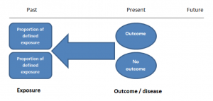
Figure 1. Case-control study design.
Cases should be selected based on objective inclusion and exclusion criteria from a reliable source such as a disease registry. An inherent issue with selecting cases is that a certain proportion of those with the disease would not have a formal diagnosis, may not present for medical care, may be misdiagnosed or may have died before getting a diagnosis. Regardless of how the cases are selected, they should be representative of the broader disease population that you are investigating to ensure generalisability.
Case-control studies should include two groups that are identical EXCEPT for their outcome / disease status.
As such, controls should also be selected carefully. It is possible to match controls to the cases selected on the basis of various factors (e.g. age, sex) to ensure these do not confound the study results. It may even increase statistical power and study precision by choosing up to three or four controls per case (2).
Case-controls can provide fast results and they are cheaper to perform than most other studies. The fact that the analysis is retrospective, allows rare diseases or diseases with long latency periods to be investigated. Furthermore, you can assess multiple exposures to get a better understanding of possible risk factors for the defined outcome / disease.
Nevertheless, as case-controls are retrospective, they are more prone to bias. One of the main examples is recall bias. Often case-control studies require the participants to self-report their exposure to a certain factor. Recall bias is the systematic difference in how the two groups may recall past events e.g. in a study investigating stillbirth, a mother who experienced this may recall the possible contributing factors a lot more vividly than a mother who had a healthy birth.
A summary of the pros and cons of case-control studies are provided in Table 1.
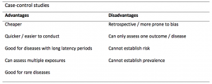
Table 1. Advantages and disadvantages of case-control studies.
Cohort studies
Cohort studies can be retrospective or prospective. Retrospective cohort studies are NOT the same as case-control studies.
In retrospective cohort studies, the exposure and outcomes have already happened. They are usually conducted on data that already exists (from prospective studies) and the exposures are defined before looking at the existing outcome data to see whether exposure to a risk factor is associated with a statistically significant difference in the outcome development rate.
Prospective cohort studies are more common. People are recruited into cohort studies regardless of their exposure or outcome status. This is one of their important strengths. People are often recruited because of their geographical area or occupation, for example, and researchers can then measure and analyse a range of exposures and outcomes.
The study then follows these participants for a defined period to assess the proportion that develop the outcome/disease of interest. See Figure 2 for a pictorial representation of a cohort study design. Therefore, cohort studies are good for assessing prognosis, risk factors and harm. The outcome measure in cohort studies is usually a risk ratio / relative risk (RR).
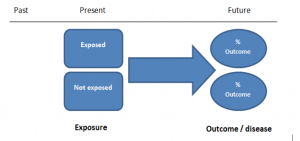
Figure 2. Cohort study design.
Cohort studies should include two groups that are identical EXCEPT for their exposure status.
As a result, both exposed and unexposed groups should be recruited from the same source population. Another important consideration is attrition. If a significant number of participants are not followed up (lost, death, dropped out) then this may impact the validity of the study. Not only does it decrease the study’s power, but there may be attrition bias – a significant difference between the groups of those that did not complete the study.
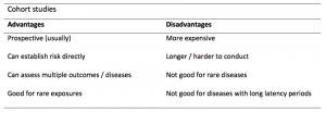
Cohort studies can assess a range of outcomes allowing an exposure to be rigorously assessed for its impact in developing disease. Additionally, they are good for rare exposures, e.g. contact with a chemical radiation blast.
Whilst cohort studies are useful, they can be expensive and time-consuming, especially if a long follow-up period is chosen or the disease itself is rare or has a long latency.
A summary of the pros and cons of cohort studies are provided in Table 2.
The Strengthening of Reporting of Observational Studies in Epidemiology Statement (STROBE)
STROBE provides a checklist of important steps for conducting these types of studies, as well as acting as best-practice reporting guidelines (3). Both case-control and cohort studies are observational, with varying advantages and disadvantages. However, the most important factor to the quality of evidence these studies provide, is their methodological quality.
- Song, J. and Chung, K. Observational Studies: Cohort and Case-Control Studies . Plastic and Reconstructive Surgery.  2010 Dec;126(6):2234-2242.
- Ury HK. Efficiency of case-control studies with multiple controls per case: Continuous or dichotomous data . Biometrics . 1975 Sep;31(3):643–649.
- von Elm E, Altman DG, Egger M, Pocock SJ, Gøtzsche PC, Vandenbroucke JP; STROBE Initiative. The Strengthening the Reporting of Observational Studies in Epidemiology (STROBE) statement: guidelines for reporting observational studies.  Lancet 2007 Oct;370(9596):1453-14577. PMID: 18064739.

Saul Crandon
Leave a reply cancel reply.
Your email address will not be published. Required fields are marked *
Save my name, email, and website in this browser for the next time I comment.
No Comments on Case-control and Cohort studies: A brief overview

Very well presented, excellent clarifications. Has put me right back into class, literally!

Very clear and informative! Thank you.

very informative article.

Thank you for the easy to understand blog in cohort studies. I want to follow a group of people with and without a disease to see what health outcomes occurs to them in future such as hospitalisations, diagnoses, procedures etc, as I have many health outcomes to consider, my questions is how to make sure these outcomes has not occurred before the “exposure disease”. As, in cohort studies we are looking at incidence (new) cases, so if an outcome have occurred before the exposure, I can leave them out of the analysis. But because I am not looking at a single outcome which can be checked easily and if happened before exposure can be left out. I have EHR data, so all the exposure and outcome have occurred. my aim is to check the rates of different health outcomes between the exposed)dementia) and unexposed(non-dementia) individuals.

Very helpful information

Thanks for making this subject student friendly and easier to understand. A great help.

Thanks a lot. It really helped me to understand the topic. I am taking epidemiology class this winter, and your paper really saved me.
Happy new year.

Wow its amazing n simple way of briefing ,which i was enjoyed to learn this.its very easy n quick to pick ideas .. Thanks n stay connected

Saul you absolute melt! Really good work man

am a student of public health. This information is simple and well presented to the point. Thank you so much.

very helpful information provided here

really thanks for wonderful information because i doing my bachelor degree research by survival model

Quite informative thank you so much for the info please continue posting. An mph student with Africa university Zimbabwe.

Thank you this was so helpful amazing

Apreciated the information provided above.

So clear and perfect. The language is simple and superb.I am recommending this to all budding epidemiology students. Thanks a lot.

Great to hear, thank you AJ!

I have recently completed an investigational study where evidence of phlebitis was determined in a control cohort by data mining from electronic medical records. We then introduced an intervention in an attempt to reduce incidence of phlebitis in a second cohort. Again, results were determined by data mining. This was an expedited study, so there subjects were enrolled in a specific cohort based on date(s) of the drug infused. How do I define this study? Thanks so much.

thanks for the information and knowledge about observational studies. am a masters student in public health/epidemilogy of the faculty of medicines and pharmaceutical sciences , University of Dschang. this information is very explicit and straight to the point

Very much helpful
Subscribe to our newsletter
You will receive our monthly newsletter and free access to Trip Premium.
Related Articles

Cluster Randomized Trials: Concepts
This blog summarizes the concepts of cluster randomization, and the logistical and statistical considerations while designing a cluster randomized controlled trial.

Expertise-based Randomized Controlled Trials
This blog summarizes the concepts of Expertise-based randomized controlled trials with a focus on the advantages and challenges associated with this type of study.

An introduction to different types of study design
Conducting successful research requires choosing the appropriate study design. This article describes the most common types of designs conducted by researchers.
Study Design 101: Case Control Study
- Case Report
- Case Control Study
- Cohort Study
- Randomized Controlled Trial
- Practice Guideline
- Systematic Review
- Meta-Analysis
- Helpful Formulas
- Finding Specific Study Types
A study that compares patients who have a disease or outcome of interest (cases) with patients who do not have the disease or outcome (controls), and looks back retrospectively to compare how frequently the exposure to a risk factor is present in each group to determine the relationship between the risk factor and the disease.
Case control studies are observational because no intervention is attempted and no attempt is made to alter the course of the disease. The goal is to retrospectively determine the exposure to the risk factor of interest from each of the two groups of individuals: cases and controls. These studies are designed to estimate odds.
Case control studies are also known as "retrospective studies" and "case-referent studies."
- Good for studying rare conditions or diseases
- Less time needed to conduct the study because the condition or disease has already occurred
- Lets you simultaneously look at multiple risk factors
- Useful as initial studies to establish an association
- Can answer questions that could not be answered through other study designs
Disadvantages
- Retrospective studies have more problems with data quality because they rely on memory and people with a condition will be more motivated to recall risk factors (also called recall bias).
- Not good for evaluating diagnostic tests because it's already clear that the cases have the condition and the controls do not
- It can be difficult to find a suitable control group
Design pitfalls to look out for
Care should be taken to avoid confounding, which arises when an exposure and an outcome are both strongly associated with a third variable. Controls should be subjects who might have been cases in the study but are selected independent of the exposure. Cases and controls should also not be "over-matched."
Is the control group appropriate for the population? Does the study use matching or pairing appropriately to avoid the effects of a confounding variable? Does it use appropriate inclusion and exclusion criteria?
Fictitious Example
There is a suspicion that zinc oxide, the white non-absorbent sunscreen traditionally worn by lifeguards is more effective at preventing sunburns that lead to skin cancer than absorbent sunscreen lotions. A case-control study was conducted to investigate if exposure to zinc oxide is a more effective skin cancer prevention measure. The study involved comparing a group of former lifeguards that had developed cancer on their cheeks and noses (cases) to a group of lifeguards without this type of cancer (controls) and assess their prior exposure to zinc oxide or absorbent sunscreen lotions.
This study would be retrospective in that the former lifeguards would be asked to recall which type of sunscreen they used on their face and approximately how often. This could be either a matched or unmatched study, but efforts would need to be made to ensure that the former lifeguards are of the same average age, and lifeguarded for a similar number of seasons and amount of time per season.
Real-life Examples
Boubekri, M., Cheung, I., Reid, K., Wang, C., & Zee, P. (2014). Impact of windows and daylight exposure on overall health and sleep quality of office workers: a case-control pilot study. Journal of Clinical Sleep Medicine : JCSM : Official Publication of the American Academy of Sleep Medicine, 10 (6), 603-611. https://doi.org/10.5664/jcsm.3780
This pilot study explored the impact of exposure to daylight on the health of office workers (measuring well-being and sleep quality subjectively, and light exposure, activity level and sleep-wake patterns via actigraphy). Individuals with windows in their workplaces had more light exposure, longer sleep duration, and more physical activity. They also reported a better scores in the areas of vitality and role limitations due to physical problems, better sleep quality and less sleep disturbances.
Togha, M., Razeghi Jahromi, S., Ghorbani, Z., Martami, F., & Seifishahpar, M. (2018). Serum Vitamin D Status in a Group of Migraine Patients Compared With Healthy Controls: A Case-Control Study. Headache, 58 (10), 1530-1540. https://doi.org/10.1111/head.13423
This case-control study compared serum vitamin D levels in individuals who experience migraine headaches with their matched controls. Studied over a period of thirty days, individuals with higher levels of serum Vitamin D was associated with lower odds of migraine headache.
Related Formulas
- Odds ratio in an unmatched study
- Odds ratio in a matched study
Related Terms
A patient with the disease or outcome of interest.
Confounding
When an exposure and an outcome are both strongly associated with a third variable.
A patient who does not have the disease or outcome.
Matched Design
Each case is matched individually with a control according to certain characteristics such as age and gender. It is important to remember that the concordant pairs (pairs in which the case and control are either both exposed or both not exposed) tell us nothing about the risk of exposure separately for cases or controls.
Observed Assignment
The method of assignment of individuals to study and control groups in observational studies when the investigator does not intervene to perform the assignment.
Unmatched Design
The controls are a sample from a suitable non-affected population.
Now test yourself!
1. Case Control Studies are prospective in that they follow the cases and controls over time and observe what occurs.
a) True b) False
2. Which of the following is an advantage of Case Control Studies?
a) They can simultaneously look at multiple risk factors. b) They are useful to initially establish an association between a risk factor and a disease or outcome. c) They take less time to complete because the condition or disease has already occurred. d) b and c only e) a, b, and c
Evidence Pyramid - Navigation
- Meta- Analysis
- Case Reports
- << Previous: Case Report
- Next: Cohort Study >>

- Last Updated: Sep 25, 2023 10:59 AM
- URL: https://guides.himmelfarb.gwu.edu/studydesign101

- Himmelfarb Intranet
- Privacy Notice
- Terms of Use
- GW is committed to digital accessibility. If you experience a barrier that affects your ability to access content on this page, let us know via the Accessibility Feedback Form .
- Himmelfarb Health Sciences Library
- 2300 Eye St., NW, Washington, DC 20037
- Phone: (202) 994-2850
- [email protected]
- https://himmelfarb.gwu.edu

An official website of the United States government
The .gov means it’s official. Federal government websites often end in .gov or .mil. Before sharing sensitive information, make sure you’re on a federal government site.
The site is secure. The https:// ensures that you are connecting to the official website and that any information you provide is encrypted and transmitted securely.
- Publications
- Account settings
- My Bibliography
- Collections
- Citation manager
Save citation to file
Email citation, add to collections.
- Create a new collection
- Add to an existing collection
Add to My Bibliography
Your saved search, create a file for external citation management software, your rss feed.
- Search in PubMed
- Search in NLM Catalog
- Add to Search
A Practical Overview of Case-Control Studies in Clinical Practice
Affiliations.
- 1 Department of Quantitative Health Sciences, Lerner Research Institute, Cleveland Clinic, Cleveland, OH; Center for Surgery and Public Health, Brigham and Women's Hospital, Harvard Medical School, Boston, MA. Electronic address: [email protected].
- 2 Department of Quantitative Health Sciences, Lerner Research Institute, Cleveland Clinic, Cleveland, OH; Department of Population and Quantitative Health Sciences, Case Western Reserve University, School of Medicine, Cleveland, OH.
- 3 Department of Statistics, University of Missouri, Columbia, MO.
- PMID: 32658653
- DOI: 10.1016/j.chest.2020.03.009
Case-control studies are one of the major observational study designs for performing clinical research. The advantages of these study designs over other study designs are that they are relatively quick to perform, economical, and easy to design and implement. Case-control studies are particularly appropriate for studying disease outbreaks, rare diseases, or outcomes of interest. This article describes several types of case-control designs, with simple graphical displays to help understand their differences. Study design considerations are reviewed, including sample size, power, and measures associated with risk factors for clinical outcomes. Finally, we discuss the advantages and disadvantages of case-control studies and provide a checklist for authors and a framework of considerations to guide reviewers' comments.
Keywords: OR; case-cohort; case-crossover; matching; nested case-control; relative risk.
Copyright © 2020 American College of Chest Physicians. Published by Elsevier Inc. All rights reserved.
PubMed Disclaimer
Similar articles
- Study Types in Orthopaedics Research: Is My Study Design Appropriate for the Research Question? Zaniletti I, Devick KL, Larson DR, Lewallen DG, Berry DJ, Maradit Kremers H. Zaniletti I, et al. J Arthroplasty. 2022 Oct;37(10):1939-1944. doi: 10.1016/j.arth.2022.05.028. Epub 2022 Sep 6. J Arthroplasty. 2022. PMID: 36162926 Free PMC article.
- Database Research for Pediatric Infectious Diseases. Kronman MP, Gerber JS, Newland JG, Hersh AL. Kronman MP, et al. J Pediatric Infect Dis Soc. 2015 Jun;4(2):143-50. doi: 10.1093/jpids/piv007. Epub 2015 Mar 5. J Pediatric Infect Dis Soc. 2015. PMID: 26407414 Review.
- Observational and interventional study design types; an overview. Thiese MS. Thiese MS. Biochem Med (Zagreb). 2014;24(2):199-210. doi: 10.11613/BM.2014.022. Epub 2014 Jun 15. Biochem Med (Zagreb). 2014. PMID: 24969913 Free PMC article. Review.
- [Hybrid designs in studies]. Mandiracioğlu A. Mandiracioğlu A. Turkiye Parazitol Derg. 2009;33(3):227-31. Turkiye Parazitol Derg. 2009. PMID: 19851970 Turkish.
- Review of guidelines for good practice in decision-analytic modelling in health technology assessment. Philips Z, Ginnelly L, Sculpher M, Claxton K, Golder S, Riemsma R, Woolacoot N, Glanville J. Philips Z, et al. Health Technol Assess. 2004 Sep;8(36):iii-iv, ix-xi, 1-158. doi: 10.3310/hta8360. Health Technol Assess. 2004. PMID: 15361314 Review.
- Factors Associated with Obstetric Anal Sphincter Injury During Vacuum-Assisted Vaginal Delivery. Chill HH, Dick A, Zarka W, Vilk Ayalon N, Rosenbloom JI, Shveiky D, Karavani G. Chill HH, et al. Int Urogynecol J. 2024 May 4. doi: 10.1007/s00192-024-05785-5. Online ahead of print. Int Urogynecol J. 2024. PMID: 38703223
- Association between statin use and the risk for idiopathic pulmonary fibrosis and its prognosis: a nationwide, population-based study. Park J, Lee CH, Han K, Choi SM. Park J, et al. Sci Rep. 2024 Apr 2;14(1):7805. doi: 10.1038/s41598-024-58417-9. Sci Rep. 2024. PMID: 38565856 Free PMC article.
- Letter to the Editor: Cross-Sectional Study for Investigation of the Association Between Modifiable Risk Factors and Gastrointestinal Cancers at a Tertiary Hospital in Ghana. Kumar A, Mansoor J, Sadiq H. Kumar A, et al. Cancer Control. 2024 Jan-Dec;31:10732748241233957. doi: 10.1177/10732748241233957. Cancer Control. 2024. PMID: 38365572 Free PMC article. No abstract available.
- Tasks and Experiences of the Prospective, Longitudinal, Multicenter MoMar (Molecular Markers) Study for the Early Detection of Mesothelioma in Individuals Formerly Exposed to Asbestos Using Liquid Biopsies. Weber DG, Casjens S, Wichert K, Lehnert M, Taeger D, Rihs HP, Brüning T, Johnen G, The MoMar Study Group. Weber DG, et al. Cancers (Basel). 2023 Dec 18;15(24):5896. doi: 10.3390/cancers15245896. Cancers (Basel). 2023. PMID: 38136442 Free PMC article.
- How to use the Surveillance, Epidemiology, and End Results (SEER) data: research design and methodology. Che WQ, Li YJ, Tsang CK, Wang YJ, Chen Z, Wang XY, Xu AD, Lyu J. Che WQ, et al. Mil Med Res. 2023 Oct 31;10(1):50. doi: 10.1186/s40779-023-00488-2. Mil Med Res. 2023. PMID: 37899480 Free PMC article. Review.
Publication types
- Search in MeSH
LinkOut - more resources
Full text sources.
- Elsevier Science
- Ovid Technologies, Inc.
- Citation Manager
NCBI Literature Resources
MeSH PMC Bookshelf Disclaimer
The PubMed wordmark and PubMed logo are registered trademarks of the U.S. Department of Health and Human Services (HHS). Unauthorized use of these marks is strictly prohibited.
Quantitative study designs: Case Control
Quantitative study designs.
- Introduction
- Cohort Studies
- Randomised Controlled Trial
Case Control
- Cross-Sectional Studies
- Study Designs Home
In a Case-Control study there are two groups of people: one has a health issue (Case group), and this group is “matched” to a Control group without the health issue based on characteristics like age, gender, occupation. In this study type, we can look back in the patient’s histories to look for exposure to risk factors that are common to the Case group, but not the Control group. It was a case-control study that demonstrated a link between carcinoma of the lung and smoking tobacco . These studies estimate the odds between the exposure and the health outcome, however they cannot prove causality. Case-Control studies might also be referred to as retrospective or case-referent studies.
Stages of a Case-Control study
This diagram represents taking both the case (disease) and the control (no disease) groups and looking back at their histories to determine their exposure to possible contributing factors. The researchers then determine the likelihood of those factors contributing to the disease.
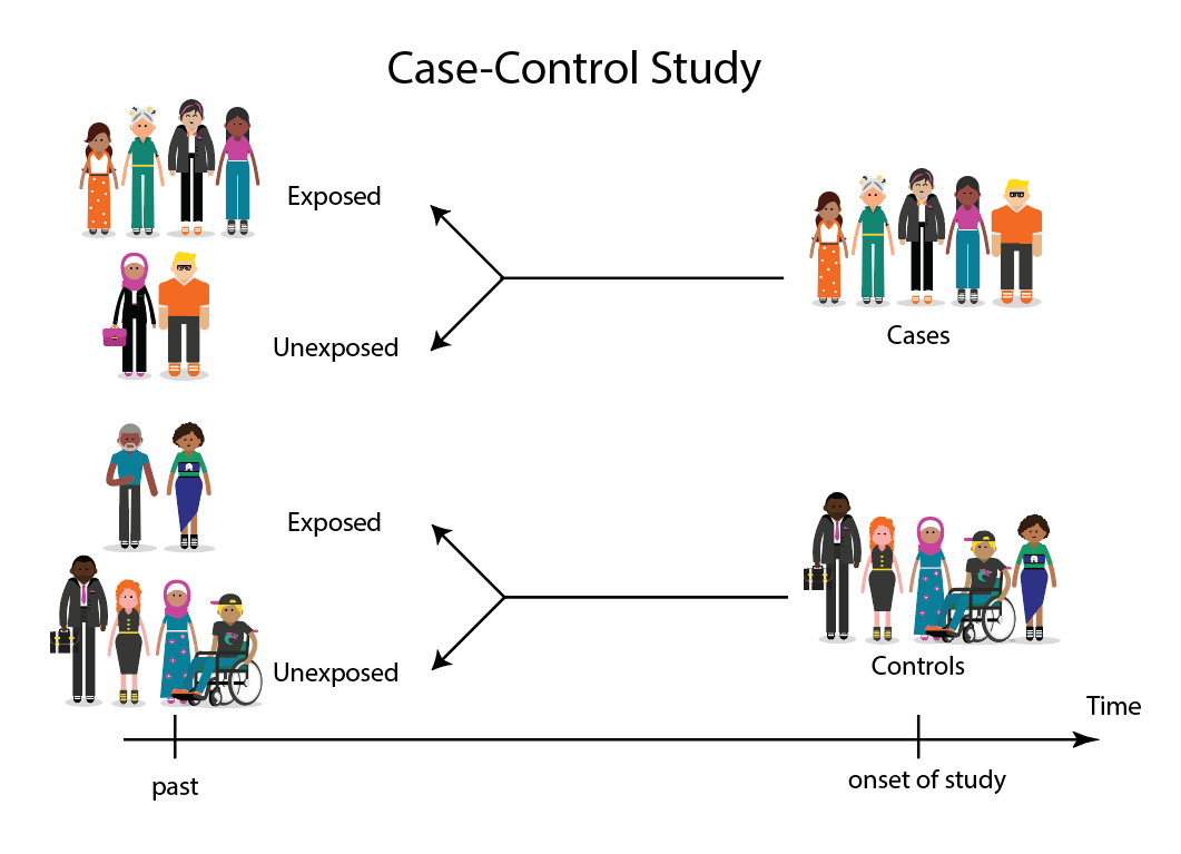
(FOR ACCESSIBILITY: A case control study is likely to show that most, but not all exposed people end up with the health issue, and some unexposed people may also develop the health issue)
Which Clinical Questions does Case-Control best answer?
Case-Control studies are best used for Prognosis questions.
For example: Do anticholinergic drugs increase the risk of dementia in later life? (See BMJ Case-Control study Anticholinergic drugs and risk of dementia: case-control study )
What are the advantages and disadvantages to consider when using Case-Control?
* Confounding occurs when the elements of the study design invalidate the result. It is usually unintentional. It is important to avoid confounding, which can happen in a few ways within Case-Control studies. This explains why it is lower in the hierarchy of evidence, superior only to Case Studies.
What does a strong Case-Control study look like?
A strong study will have:
- Well-matched controls, similar background without being so similar that they are likely to end up with the same health issue (this can be easier said than done since the risk factors are unknown).
- Detailed medical histories are available, reducing the emphasis on a patient’s unreliable recall of their potential exposures.
What are the pitfalls to look for?
- Poorly matched or over-matched controls. Poorly matched means that not enough factors are similar between the Case and Control. E.g. age, gender, geography. Over-matched conversely means that so many things match (age, occupation, geography, health habits) that in all likelihood the Control group will also end up with the same health issue! Either of these situations could cause the study to become ineffective.
- Selection bias: Selection of Controls is biased. E.g. All Controls are in the hospital, so they’re likely already sick, they’re not a true sample of the wider population.
- Cases include persons showing early symptoms who never ended up having the illness.
Critical appraisal tools
To assist with critically appraising case control studies there are some tools / checklists you can use.
CASP - Case Control Checklist
JBI – Critical appraisal checklist for case control studies
CEBMA – Centre for Evidence Based Management – Critical appraisal questions (focus on leadership and management)
STROBE - Observational Studies checklists includes Case control
SIGN - Case-Control Studies Checklist
Real World Examples
Smoking and carcinoma of the lung; preliminary report
- Doll, R., & Hill, A. B. (1950). Smoking and carcinoma of the lung; preliminary report. British Medical Journal , 2 (4682), 739–748. Retrieved from https://www.ncbi.nlm.nih.gov/pmc/articles/PMC2038856/
- Key Case-Control study linking tobacco smoking with lung cancer
- Notes a marked increase in incidence of Lung Cancer disproportionate to population growth.
- 20 London Hospitals contributed current Cases of lung, stomach, colon and rectum cancer via admissions, house-physician and radiotherapy diagnosis, non-cancer Controls were selected at each hospital of the same-sex and within 5 year age group of each.
- 1732 Cases and 743 Controls were interviewed for social class, gender, age, exposure to urban pollution, occupation and smoking habits.
- It was found that continued smoking from a younger age and smoking a greater number of cigarettes correlated with incidence of lung cancer.
Anticholinergic drugs and risk of dementia: case-control study
- Richardson, K., Fox, C., Maidment, I., Steel, N., Loke, Y. K., Arthur, A., . . . Savva, G. M. (2018). Anticholinergic drugs and risk of dementia: case-control study. BMJ , 361, k1315. Retrieved from http://www.bmj.com/content/361/bmj.k1315.abstract .
- A recent study linking the duration and level of exposure to Anticholinergic drugs and subsequent onset of dementia.
- Anticholinergic Cognitive Burden (ACB) was estimated in various drugs, the higher the exposure (measured as the ACB score) the greater likeliness of onset of dementia later in life.
- Antidepressant, urological, and antiparkinson drugs with an ACB score of 3 increased the risk of dementia. Gastrointestinal drugs with an ACB score of 3 were not strongly linked with onset of dementia.
- Tricyclic antidepressants such as Amitriptyline have an ACB score of 3 and are an example of a common area of concern.
Omega-3 deficiency associated with perinatal depression: Case-Control study
- Rees, A.-M., Austin, M.-P., Owen, C., & Parker, G. (2009). Omega-3 deficiency associated with perinatal depression: Case control study. Psychiatry Research , 166(2), 254-259. Retrieved from http://www.sciencedirect.com/science/article/pii/S0165178107004398 .
- During pregnancy women lose Omega-3 polyunsaturated fatty acids to the developing foetus.
- There is a known link between Omgea-3 depletion and depression
- Sixteen depressed and 22 non-depressed women were recruited during their third trimester
- High levels of Omega-3 were associated with significantly lower levels of depression.
- Women with low levels of Omega-3 were six times more likely to be depressed during pregnancy.
References and Further Reading
Doll, R., & Hill, A. B. (1950). Smoking and carcinoma of the lung; preliminary report. British Medical Journal, 2(4682), 739–748. Retrieved from https://www.ncbi.nlm.nih.gov/pmc/articles/PMC2038856/
Greenhalgh, Trisha. How to Read a Paper: the Basics of Evidence-Based Medicine, John Wiley & Sons, Incorporated, 2014. ProQuest Ebook Central, http://ebookcentral.proquest.com/lib/deakin/detail.action?docID=1642418 .
Himmelfarb Health Sciences Library. (2019). Study Design 101: Case-Control Study. Retrieved from https://himmelfarb.gwu.edu/tutorials/studydesign101/casecontrols.cfm
Hoffmann, T., Bennett, S., & Del Mar, C. (2017). Evidence-Based Practice Across the Health Professions (Third edition. ed.): Elsevier.
Lewallen, S., & Courtright, P. (1998). Epidemiology in practice: case-control studies. Community Eye Health, 11(28), 57. https://www.ncbi.nlm.nih.gov/pmc/articles/PMC1706071/
Pelham, B. W. a., & Blanton, H. (2013). Conducting research in psychology : measuring the weight of smoke /Brett W. Pelham, Hart Blanton (Fourth edition. ed.): Wadsworth Cengage Learning.
Rees, A.-M., Austin, M.-P., Owen, C., & Parker, G. (2009). Omega-3 deficiency associated with perinatal depression: Case control study. Psychiatry Research, 166(2), 254-259. Retrieved from http://www.sciencedirect.com/science/article/pii/S0165178107004398
Richardson, K., Fox, C., Maidment, I., Steel, N., Loke, Y. K., Arthur, A., … Savva, G. M. (2018). Anticholinergic drugs and risk of dementia: case-control study. BMJ, 361, k1315. Retrieved from http://www.bmj.com/content/361/bmj.k1315.abstract
Statistics How To. (2019). Case-Control Study: Definition, Real Life Examples. Retrieved from https://www.statisticshowto.com/case-control-study/
- << Previous: Randomised Controlled Trial
- Next: Cross-Sectional Studies >>
- Last Updated: Jun 13, 2024 10:34 AM
- URL: https://deakin.libguides.com/quantitative-study-designs

Case-Control Studies
- 1
- | 2
- | 3
- | 4
- | 5
- | 6
- | 7
- | 8

Selecting & Defining Cases and Controls
The "case" definition, sources of cases, selection of the controls.

E pi_Tools.XLSX
All Modules
Careful thought should be given to the case definition to be used. If the definition is too broad or vague, it is easier to capture people with the outcome of interest, but a loose case definition will also capture people who do not have the disease. On the other hand, an overly restrictive case definition is employed, fewer cases will be captured, and the sample size may be limited. Investigators frequently wrestle with this problem during outbreak investigations. Initially, they will often use a somewhat broad definition in order to identify potential cases. However, as an outbreak investigation progresses, there is a tendency to narrow the case definition to make it more precise and specific, for example by requiring confirmation of the diagnosis by laboratory testing. In general, investigators conducting case-control studies should thoughtfully construct a definition that is as clear and specific as possible without being overly restrictive.
Investigators studying chronic diseases generally prefer newly diagnosed cases, because they tend to be more motivated to participate, may remember relevant exposures more accurately, and because it avoids complicating factors related to selection of longer duration (i.e., prevalent) cases. However, it is sometimes impossible to have an adequate sample size if only recent cases are enrolled.
Typical sources for cases include:
- Patient rosters at medical facilities
- Death certificates
- Disease registries (e.g., cancer or birth defect registries; the SEER Program [Surveillance, Epidemiology and End Results] is a federally funded program that identifies newly diagnosed cases of cancer in population-based registries across the US )
- Cross-sectional surveys (e.g., NHANES, the National Health and Nutrition Examination Survey)
As noted above, it is always useful to think of a case-control study as being nested within some sort of a cohort, i.e., a source population that produced the cases that were identified and enrolled. In view of this there are two key principles that should be followed in selecting controls:
- The comparison group ("controls") should be representative of the source population that produced the cases.
- The "controls" must be sampled in a way that is independent of the exposure, meaning that their selection should not be more (or less) likely if they have the exposure of interest.
If either of these principles are not adhered to, selection bias can result (as discussed in detail in the module on Bias ).

Note that in the earlier example of a case-control study conducted in the Massachusetts population, we specified that our sampling method was random so that exposed and unexposed members of the population had an equal chance of being selected. Therefore, we would expect that about 1,000 would be exposed and 5,000 unexposed (the same ratio as in the whole population), and came up with an odds ratio that was same as the hypothetical risk ratio we would have had if we had collected exposure information from the whole population of six million:
What if we had instead been more likely to sample those who were exposed, so that we instead found 1,500 exposed and 4,500 unexposed among the 6,000 controls? Then the odds ratio would have been:
This odds ratio is biased because it differs from the true odds ratio. In this case, the bias stemmed from the fact that we violated the second principle in selection of controls. Depending on which category is over or under-sampled, this type of bias can result in either an underestimate or an overestimate of the true association.
A hypothetical case-control study was conducted to determine whether lower socioeconomic status (the exposure) is associated with a higher risk of cervical cancer (the outcome). The "cases" consisted of 250 women with cervical cancer who were referred to Massachusetts General Hospital for treatment for cervical cancer. They were referred from all over the state. The cases were asked a series of questions relating to socioeconomic status (household income, employment, education, etc.). The investigators identified control subjects by going door-to-door in the community around MGH from 9:00 AM to 5:00 PM. Many residents are not home, but they persist and eventually enroll enough controls. The problem is that the controls were selected by a different mechanism than the cases, AND the selection mechanism may have tended to select individuals of different socioeconomic status, since women who were at home may have been somewhat more likely to be unemployed. In other words, the controls were more likely to be enrolled (selected) if they had the exposure of interest (lower socioeconomic status).

What is the purpose of the control group in a case-control study?
a. To provide information on the disease distribution in the population that gave rise to the cases.
b. To provide information on the exposure distribution in the population that gave rise to the cases.
return to top | previous page | next page
Content ©2016. All Rights Reserved. Date last modified: June 7, 2016. Wayne W. LaMorte, MD, PhD, MPH
- Open access
- Published: 26 June 2024
Characterization of bacterial and viral pathogens in the respiratory tract of children with HIV-associated chronic lung disease: a case–control study
- Prince K. Mushunje 1 na1 ,
- Felix S. Dube 1 , 2 na1 ,
- Courtney Olwagen 3 ,
- Shabir Madhi 3 , 4 ,
- Jon Ø Odland 5 , 6 , 7 ,
- Rashida A. Ferrand 8 , 9 ,
- Mark P. Nicol 10 ,
- Regina E. Abotsi 1 , 11 &
The BREATHE study team
BMC Infectious Diseases volume 24 , Article number: 637 ( 2024 ) Cite this article
175 Accesses
Metrics details
Introduction
Chronic lung disease is a major cause of morbidity in African children with HIV infection; however, the microbial determinants of HIV-associated chronic lung disease (HCLD) remain poorly understood. We conducted a case–control study to investigate the prevalence and densities of respiratory microbes among pneumococcal conjugate vaccine (PCV)-naive children with (HCLD +) and without HCLD (HCLD-) established on antiretroviral treatment (ART).
Nasopharyngeal swabs collected from HCLD + (defined as forced-expiratory-volume/second < -1.0 without reversibility postbronchodilation) and age-, site-, and duration-of-ART-matched HCLD- participants aged between 6–19 years enrolled in Zimbabwe and Malawi (BREATHE trial-NCT02426112) were tested for 94 pneumococcal serotypes together with twelve bacteria, including Streptococcus pneumoniae (SP), Staphylococcus aureus (SA), Haemophilus influenzae (HI), Moraxella catarrhalis (MC), and eight viruses, including human rhinovirus (HRV), respiratory syncytial virus A or B, and human metapneumovirus, using nanofluidic qPCR (Standard BioTools formerly known as Fluidigm). Fisher's exact test and logistic regression analysis were used for between-group comparisons and risk factors associated with common respiratory microbes, respectively.
A total of 345 participants (287 HCLD + , 58 HCLD-; median age, 15.5 years [IQR = 12.8–18], females, 52%) were included in the final analysis. The prevalence of SP (40%[116/287] vs. 21%[12/58], p = 0.005) and HRV (7%[21/287] vs. 0%[0/58], p = 0.032) were higher in HCLD + participants compared to HCLD- participants. Of the participants positive for SP (116 HCLD + & 12 HCLD-), 66% [85/128] had non-PCV-13 serotypes detected. Overall, PCV-13 serotypes (4, 19A, 19F: 16% [7/43] each) and NVT 13 and 21 (9% [8/85] each) predominated. The densities of HI (2 × 10 4 genomic equivalents [GE/ml] vs. 3 × 10 2 GE/ml, p = 0.006) and MC (1 × 10 4 GE/ml vs. 1 × 10 3 GE/ml , p = 0.031) were higher in HCLD + compared to HCLD-. Bacterial codetection (≥ any 2 bacteria) was higher in the HCLD + group (36% [114/287] vs. (19% [11/58]), ( p = 0.014), with SP and HI codetection (HCLD + : 30% [86/287] vs. HCLD-: 12% [7/58], p = 0.005) predominating. Viruses (predominantly HRV) were detected only in HCLD + participants. Lastly, participants with a history of previous tuberculosis treatment were more likely to carry SP (adjusted odds ratio (aOR): 1.9 [1.1 -3.2], p = 0.021) or HI (aOR: 2.0 [1.2 – 3.3], p = 0.011), while those who used ART for ≥ 2 years were less likely to carry HI (aOR: 0.3 [0.1 – 0.8], p = 0.005) and MC (aOR: 0.4 [0.1 – 0.9], p = 0.039).
Children with HCLD + were more likely to be colonized by SP and HRV and had higher HI and MC bacterial loads in their nasopharynx. The role of SP, HI, and HRV in the pathogenesis of CLD, including how they influence the risk of acute exacerbations, should be studied further.
Trial registration
The BREATHE trial (ClinicalTrials.gov Identifier: NCT02426112 , registered date: 24 April 2015).
Peer Review reports
In 2019, over 2.8 million children and adolescents were living with HIV globally, 90% in sub-Saharan Africa [ 1 ]. Respiratory infections remain the most common manifestation of HIV among these children and adolescents [ 2 , 3 ]. The scale-up of antiretroviral therapy (ART) has increased survival so that growing numbers of children are entering adulthood. In addition, ART has resulted in a reduction in the rate of respiratory disorders, including tuberculosis and lymphocytic interstitial pneumonitis [ 4 , 5 , 6 , 7 ]. However, studies in sub-Saharan Africa revealed that approximately 30% of HIV-infected older children experience chronic respiratory symptoms, including chronic cough and reduced tolerance to exercise, which often leads to presumptive tuberculosis treatment [ 8 ]. The clinical and radiological picture of this chronic lung disease is consistent with small airway disease, predominantly constrictive obliterative bronchiolitis [ 9 ].
The pathogenesis of this condition is incompletely understood. It is speculated that HIV-induced chronic inflammation and dysregulated immune activation may play a role [ 10 , 11 , 12 ]. A previous study of older children with HIV-associated chronic lung disease (HCLD) conducted by our group demonstrated that there was increased inflammatory activation in children with HCLD (HCLD +) compared to their HIV-infected counterparts without HCLD (HCLD-) [ 13 ]. In the same cohort, there was an association between the carriage of specific bacteria in the nasopharynx and HCLD [ 14 ]. Specifically, we observed that older children with HCLD were more likely to be colonized with Streptococcus pneumoniae (SP) and Moraxella catarrhalis (MC) than their HCLD- counterparts [ 14 ]. The study utilized bacterial culture, which is limited by viability and a narrow spectrum of culturable bacterial species. Although we observed that SP was associated with HCLD, we did not investigate the specific serotypes that may be involved in this condition, which is important to inform pneumococcal immunization. Furthermore, the prevalence of respiratory viruses was also not studied.
Viruses facilitate bacterial infections in the host through various mechanisms, including damaging the respiratory epithelium, modifying the immune response, and altering cell membranes [ 15 ]. Coinfection of viruses and bacteria leads to increased bacterial load, thus making individuals more susceptible to complications related to upper respiratory tract infections [ 16 ]. Prior to COVID-19, respiratory syncytial virus, influenza virus and human rhinovirus (HRV) were the most common causative agents of upper respiratory infection and have been linked to exacerbations of COPD [ 17 , 18 ], asthma development [ 17 ], and severe bronchiolitis in children [ 19 , 20 , 21 ].
To overcome these limitations, we investigated the prevalence of respiratory pathogens in both HCLD + and HCLD- participants using real-time quantitative polymerase chain reaction (qPCR) to detect and quantify a large number of bacterial and viral targets and elucidate common SP serotypes (94 serotypes). We also assessed clinical and sociodemographic factors associated with microbial carriage and density.
Materials and methods
Study design, population, and setting.
This case–control study was nested within the BREATHE trial (ClinicalTrials.gov Identifier: NCT02426112, registered date: 24 April 2015) investigating whether azithromycin therapy could improve lung function and reduce the risk of exacerbations among children with HCLD [ 22 ]. BREATHE was a two-site, double-blinded, placebo-controlled, individually randomized trial conducted in Harare (Zimbabwe) and Blantyre (Malawi). The study setting, population, and trial procedures are described elsewhere [ 22 , 23 , 24 ]. Briefly, we enrolled perinatally HIV-infected participants aged 6 – 19 years with HCLD. HCLD was defined as a forced expiratory volume in 1 s (FEV1) z score < -1, with no reversibility (< 12% improvement in FEV1 after salbutamol 200 µg inhaled using a spacer) [ 22 ]. A group of perinatally HIV-infected children without HCLD (FEV1 z score > 0) was also recruited at the same time as the enrollment of trial participants using frequency matching for site, sex, age, and duration of ART to serve as a comparison group for pathogenesis studies. Both groups were on ART for at least six months. All participants were most likely not vaccinated due to the introduction of PCV13 in 2012 in Zimbabwe [ 25 ] and in Malawi in 2011 [ 26 ], making them ineligible for vaccination at that time because of their older age. Swabs were collected between June 1, 2016 and September 31, 2019. Sociodemographic data and clinical history were recorded through an interviewer-administered questionnaire.
Nasopharyngeal swab collection
Nasopharyngeal swabs were collected at baseline from all participants using sterile flocked flexible nylon swabs (Copan Italia, Brescia, Italy). Swabs were immediately immersed in 1 mL PrimeStore® Molecular Transport Medium (MTM) (Longhorn Vaccines & Diagnostics LLC, Bethesda, USA), transported on ice and stored at -80 °C at the diagnostic laboratory at each site. PrimeStore® MTM was used because it is a medium optimized for transporting and storing samples for molecular analyses; it also inactivates potential pathogens and stabilizes nucleic acids [ 27 ]. The samples were batched and transported on dry ice to Cape Town, South Africa, where they were stored at -80 °C until further processing.
Total nucleic acid extraction
Total nucleic acid (TNA) extraction for microbial identification was conducted on NP swabs stored in Primestore® MTM. Briefly, the samples were thawed and vortexed for 10 s, and 400 µl aliquots were transferred into ZR BashingBead™ Lysis Tubes containing 0.5 mm beads (catalog no. ZR S6002–50, Zymo Research Corp., Irvine, CA, United States) for the mechanical lysis steps. Lysis was conducted on a Qiagen Tissue lyser LTTM (Qiagen, FRITSCH GmbH, Idar-Oberstein, Germany) for 5 min at 50 Hz, followed by centrifugation (Eppendorf F-45–30-11, Merck KgaA, Darmstadt, Germany) for 1 min at 10,000 rpm (10,640 g). The supernatants (250 µl) were extracted using the QIAsymphony® DSP Virus/Pathogen Kit (Qiagen GmbH, Hilden, Germany) on the QIAsymphony SP/AS instrument (Qiagen GmbH, Hilden, Germany) following the manufacturer’s instructions. The total nucleic acid was eluted in 70 µl DNA elution buffer into the Elution Microtube (Qiagen GmbH, Hilden, Germany) and immediately stored at -80 °C until further analysis.
Real-time qPCR using the biomark HD system (Fluidigm assay)
Nanofluidic qPCR testing was performed at the WITS-VIDA Research Unit, Witwatersrand University, Johannesburg, South Africa as previously described [ 28 , 29 ]. Briefly, all extracts were tested for 94 SP serotypes together with 12 bacterial species (SP, HI, MC, Staphylococcus aureus [SA], Neisseria lactamica , Neisseria meningitidis , Streptococcus pyogenes , Bordetella pertussis , Bordetella holmesii , Klebsiella pneumoniae , Acinetobacter baumanii and Streptococcus oralis ), 6 HI serotypes and 8 viruses (respiratory syncytial virus A and B, human rhinovirus, influenza A and B, human parainfluenza 1 and 3, and human metapneumovirus). Furthermore, all samples were previously cultured for SP, HI, MC and SA as described elsewhere [ 14 ]. These microbial targets (Table S1) included on the nanofluidic panel might be associated with HCLD and are the most frequent pathobionts in the nasopharynx. A detailed list of these microbial targets can be found in the supplementary material (Table S1). For SP, positive samples were defined as those with a Cycle of quantification (Cq) value ≤ 36 for each serotype-specific qPCR target and positive for both Lyt A and Pia B. Negative samples were defined as those with Cq values ≥ 36 for each target.
The bacterial or serotype densities were determined following the method outlined by Downs et al . [ 28 ]. Briefly, culture controls and synthetic double-stranded DNA (dsDNA) template gene fragments (gBlocks) were included in the assay as external calibrators, reported as copy numbers or gene equivalents, respectively. A DNA library was prepared for the targeted pneumococcal serotypes or other bacterial species at an average concentration ranging from 10 3 to 10 4 CFU/ml. For assay-sets meeting the defined efficiency criteria (90–110%), the relative quantification of bacterial density was determined by extrapolating using the linear equation derived from standard curves of the calibrators (control strains and gBlocks with known densities), employing the equation and reported as log 10 genomic equivalents/ml:
Data management and statistical analysis
Clinical and sociodemographic data were electronically captured using Google NexusTM tablets (Google, Mountain View, CA, USA) running OpenDataKit software, managed on Microsoft Access databases (Microsoft, Redmond, WA, USA) and analyzed using Stata ((StataCorp, College Station, TX). Comparisons between groups were performed with the Student T test or Mann–Whitney U test for continuous data and chi-squared or Fisher’s exact tests for categorical data where appropriate with no further adjustment of multiplexity. Multivariate logistic regression, adjusting for age category, duration of ART, site, sex, height-for-age, HIV viral suppression, history of TB treatment, Medical Research Council dyspnea score and ART regimen, was used to investigate the factors associated with microbial carriage and density. The following were excluded from the multivariate model because of colinearity: Enrollment BMI-for-age z score, weight-for-age z score, and CD4 count. A p value of less than 0.05 was considered statistically significant.
Clinical and sociodemographic characteristics
The study included 345 participants, HCLD + ( n = 287) and HCLD- ( n = 58), with a median age [IQR] of 15.5 (12.8 – 18.0) years and 52% (180/345)] female (Table 1 ). The median BMI-for-age- z score for the HCLD + group was lower compared to the HCLD- group (-1.1 vs -0.4), p < 0.001. A higher proportion of the participants from the HCLD + group were previously treated for tuberculosis (31% vs. 12%, p = 0.001), stunted (49% vs . 29%, p = 0.009) and underweight (52% vs . 14%, p < 0.001) compared to the HCLD- group. A higher number of HCLD + participants were on a second-line ART (protease inhibitor-based) regimen (25% vs. 10%, p = 0.01) compared to HCLD-. Ten percent of HCLD + participants compared to HLCD- (2%) participants had an MRC dyspnea score of 3 or above. None of the participants reported smoking.
Prevalence and densities of selected nasopharyngeal microbes in participants with and without HCLD
The prevalence and median densities of selected microbes detected in the nasopharynx of HCLD + and HCLD- participants are summarized in Table 2 . The prevalence of SP colonization was significantly higher in the HCLD + group (40%, 116/278) compared to the HCLD- group (21%, 12/58; p = 0.005). However, there were no statistically significant differences between the two groups in colonization prevalence of pneumococcal serotypes covered by the 13-valent pneumococcal conjugate vaccine (PCV13 vaccine types, VT) or those not covered (non-vaccine types, NVT).
Of the 128 participants colonized with SP (116 HCLD + , 12 HCLD-), 66% (85/128) carried NVT serotypes, while 34% (43/128) carried PCV13 VT serotypes (Fig. 1 ). A total of 150 pneumococcal serotypes was detected in the 128 participants colonized with SP including 134 serotypes from the HCLD + group and 16 from the HCLD- group (Fig. 1 ). Multiple serotypes were detected in 14% (16/116) of HCLD + participants and 17% (2/12) of the HCLD- participants colonized with SP.

Pneumococcal serotypes recovered from nasopharyngeal swabs of HCLD + and HCLD- participants. Abbreviations: PCV, polysaccharide-conjugated vaccine; n, number of swabs serotyped using the fluidigm assay from the HCLD + group ( n = 116) and HCLD- group ( n = 12). Denominator for prevalence is the total number of SP serotypes grouped into PCV 13 and non-PCV 13 serotypes. Others* HCLD + group: PCV13 serotype [3 (0.7%), 5 (0.7%), 6B (0.7%), 9AV (0.7%), 4 (5.2%), Others**: HCLD + group non-PCV 13 serotype [18B (0.7%), 19 atypical (0.7%), 20 (0.7%), 23B (1.5%), 27 (0.7%), 25AF/38 (0.7%), 45 (0.7%), 29 (0.7%), 31 (0.7%), 33C (1.5%), 38 (0.7%)]; HCLD- group non-PCV13 serotype [10A (6.3%), 10B (6.3%), 22A (6.3%), 33B (6.3%)]. 15: HCLD + group non-PCV 13 serotype [15AF (3.7%), 15BC (2.2%), 15like (1.5%)]; HCLD- group non-PCV13 serotype [15like (6.3%)]. 11: HCLD + group non-PCV 13 serotype [11AD [3.7%), 11E (1.5%)]; HCLD- group non-PCV13 serotype [11E (6.3%)]
NVT serotypes predominated over PCV13 VTs in both groups, accounting for 69% (93/134) in HCLD + and 81% (13/16) in HCLD- (Fig. 1 ). While not statistically significant ( p = 0.398), the prevalence of PCV13 VT serotypes trended higher in HCLD + (31%, 41/134) compared to HCLD- (19%, 3/16).
The most common PCV13 VT serotypes in both groups were 4 (16%, 7/44), 19F (16%, 7/44), 19A (16%, 7/44), and 18C (14%, 6/44). The predominant NVTs were 13 and 21 (8% each, 8/106). There were no statistically significant differences in serotype-specific colonization prevalence between HCLD + and HCLD- groups. Likewise, the median densities of the composite NVT and PCV13 VT serotypes did not differ significantly between the two groups (Figure S1). The overall median serotype density across all samples was 8.8 genomic equivalents/ml.
There were no significant differences in the colonization prevalence of any other bacteria tested. Despite there being no difference in the colonization prevalence for both HI and MC, the mean log density was higher in the HCLD + ( 2 × 10 4− gene equivalents [GE]/ml & 1 × 10 4 GE/ml) compared to the HCLD- (3 × 10 2 GE/ml; p = 0.006 & 0.5 × 10 3 GE/ml; p = 0.031,) groups, respectively (Table 2 ). There was no significant difference in the mean log densities between the groups for the other tested bacteria. There was a low prevalence of the viruses detected amongst the group, with HRV (7% [21/287] vs . 0% [0/58], p = 0.032) detected in the HCLD + group only. The bacterial species Klebsiella pneumoniae , Neisseria meningitidis , Actinobacter baumanii , Bordetella pertussis/holmesii , and viruses influenza A, influenza B, human parainfluenza type 1 & 3, and human metapneumovirus were not detected in any participants.
Nasopharyngeal bacterial and viral co-colonization in participants with and without HCLD
Bacterial and viral co-colonization detected in HIV-infected participants with or without HCLD is summarized in Table 3 and Table S2. Bacterial detection (any) was significantly higher in HCLD + (61% [175/287]) than in HCLD- (43.1% [25/58]) ( p = 0.013). Moreover, the concurrent carriage of multiple bacterial species was higher in the HCLD + group (35.9% [103/287]) than in the HCLD- group (19% [11/58]) ( p = 0.014). The most frequent bacteria detected concurrently with SP included SP were HI (HCLD + : 30% [87/287]) vs. HCLD-: 12.1% [7/58], p = 0.013) and MC (HCLD + : 23.3% [67/287] vs. HCLD-: 12.1% [7/58], p = 0.078). Viruses were detected only in the HCLD + group (8% [23/287]), with viral and bacterial co-colonization reported in 6.6% (19/287) of HCLD + participants. To determine whether the concurrent detection of bacteria in HCLD + participants was due to a true interaction or simply by chance, we compared the observed and expected values based on marginal probabilities. The results showed that the co-colonization of SP with HI (Observed [86/287] vs Expected [50.1/287], p < 0.001); SP with MC (Observed [60/287] vs Expected [30.3/287]], p < 0.001) and MC with HI (Observed [54/287] vs Expected [32.4/287], p < 0.001]) was a result of true interactions with HCLD (Table S3).
Factors associated with carriage of selected bacteria at baseline in participants with HCLD
The results of the univariate and multivariate analyses of the clinical and sociodemographic factors associated with the carriage of SP and SA are displayed in Table 4 , while those for HI and MC are shown in Table 5 . On multivariate analysis, participants previously treated for TB (adjusted odds ratio were more likely to carry SP (aOR): 1.9 [1.1 -3.2], p = 0.021) or HI (aOR: 2.0 [1.2 – 3.3], p = 0.011). Participants on ART for ≥ 2 years (aOR: 0.3 [0.1 – 0.8], p = 0.005) and living in Zimbabwe (aOR: 0.5 [0.3 – 0.9], p = 0.026) were less likely to carry HI (Table 5 ). Similarly, MC carriage was less likely in participants who had been on ART for ≥ 2 years (aOR: 0.4 [0.1 – 0.9], p = 0.039) (Table 5 ). Participants who were attending school were more likely to carry MC (aOR: 2.5 [1.0 -6.4], p = 0.050) (Table 5 ).
In this study, we used quantitative PCR to determine the prevalence and density of bacterial and viral carriage in HIV-infected African children. As previously shown [ 14 ], microbial colonization was more frequently detected in HCLD + than HCLD- participants, with the former more likely to carry SP or HRV. Strikingly, viruses (predominantly HRV) were detected only in HCLD + children. Moreover, we observed that HCLD + participants had a higher HI and MC density than their HCLD- counterparts. The prevalence and densities of all SP serotypes tested were similar between the two groups, with more of the recovered SP serotypes (79%) being non-PCV 13. Study participants with a history of previous tuberculosis treatment were more likely to carry SP or HI, while those who used ART for ≥ 2 years were less likely to carry HI and MC. Furthermore, those living in Zimbabwe were less likely to carry HI.
The prevalence of HI in the current study in both HCLD + (43%) and HCLD- (33%) participants was higher than that observed in our previous study of the same cohort by Abotsi et al. [ 14 ] (12% and 5%, respectively). Similar studies conducted in India [ 30 ] and Zambia [ 31 ] in HIV-infected children observed similar prevalence (26% and 29%, respectively) to our current study (33%). The discrepancy in results could be attributed to the more sensitive PCR detection method used in our study compared to the culture method employed in previous studies as well as age and pathological differences.
Furthermore, HCLD + participants showed a higher density of HI than their counterparts. Previous studies have associated HI carriage in participants with other lung diseases, including asthma [ 32 ], bronchiectasis [ 33 , 34 ] and chronic obstructive pulmonary disease [ 35 , 36 , 37 ]. HI has been identified as a biomarker for predicting the response to azithromycin treatment in adults with persistent uncontrolled asthma [ 32 ]. It has also been associated with negative outcomes in children suffering from respiratory viral infections [ 38 ], including hospitalization among RSV-positive children [ 39 ]. The bacterium’s ability to invade host epithelial cells, evade host defense mechanisms, form biofilms and survive as an intracellular pathogen contributes to its pathogenic nature [ 40 ], which may suggest an important role that it may play in HCLD + pathogenesis. However, further studies are needed to further elucidate this observation.
The prevalence of carriage of SA in this study (HCLD + [6%] and HCLD- [5%]) was markedly lower than that observed using bacterial culture in the same cohort (HCLD + [23%] and HCLD- [19%]) [ 14 ]. This difference in prevalence may be related to the efficiency of the nucleic acid extraction method used. The extraction of nucleic acids requires extended and vigorous lysis steps for some bacterial species (gram-positive such as SA) compared to others (gram-negative such as HI and MC) [ 41 ]; however, for this study, although we used a rigorous extraction protocol incorporating bead-beating, the inherent complexity and resilience of the SA bacterial cell wall may have contributed to the low yield. This underscores the need for tailored approaches and ongoing refinement of extraction methods to include enzymatic lysis alternatives such as lysostaphin or lysozyme in NP swabs DNA extraction for enhanced yield. Additionally, carriage may have been influenced by the efficiency of the annealing of PCR primers [ 42 ].
High SP, HI and MC density in the nasopharynx has been associated with respiratory infections in children [ 43 , 44 ]. This is consistent with our study, where a higher HI and MC density was observed in HCLD + participants than in their HCLD- counterparts. The HCLD + participants may have a chronic lung infection, as evidenced by the isolation of bacteria from their sputum in our previous study [ 14 ]. Microbiota dominated by Haemophilus , Moraxella or Neisseria species are associated with chronic lung diseases, including chronic obstructive pulmonary disease and asthma [ 45 , 46 , 47 , 48 ]. Bhadriraju et al . [ 40 ] observed that HIV-infected children with a sputum bacteriome dominated by Haemophilus , Moraxella or Neisseria species were 1.5 times more likely to have HCLD than those with Streptococcus or Prevotella spp. [ 40 ]. These bacterial genera were also associated with enhanced inflammatory effects [ 40 ]. Interestingly, we detected Neisseria species ( N. lactamica ) in HCLD + participants only. Taken together, these findings support the important role of HI and MC in HCLD.
Our observation of a higher SP carriage in the HCLD + group than in the HCLD- group is consistent with our culture-based study of the same cohort [ 14 ]. Furthermore, SP carriage in the HCLD- participants (21%) is comparable to studies of HIV-infected children in South Africa (22.2%) [ 49 ] and Cambodia (17.6%) [ 42 , 50 ]. Nevertheless, the prevalence is higher than that observed in children living with HIV in Ethiopia (10.3%) [ 51 ] and lower than that in studies from Ghana (27.1%) and Tanzania (81%) [ 52 ]. The differences in SP prevalence observed between studies can again be related to differences in the age of participants—younger children have a higher carriage prevalence[ 31 , 52 ], socioeconomic factors [ 53 ] and the geographical location of the participants.
The prevalence of PCV 13 serotypes and densities in both study groups (HCLD + : 30.4% and HCLD-: 16.7%) did not differ significantly. The most prevalent PCV-13 serotypes were serotypes 4 (15.9%), 19F (15.9%), 19A (15.9%) and 18C (14%). A study of HIV-infected children in Malawi [ 54 ] reports 19F and 6A among the most predominant serotypes. The relatively high prevalence of serotype 19A in PCV-vaccinated children has been suggested by Kamng’ona et al . [ 54 ] to occur due to an inversion in the rmlD gene at the CPS locus. This may downregulate the rmlD gene on the CPS locus, causing an altered 19A capsule [ 55 ] that is not recognized by the PCV vaccine.
There was a higher prevalence of non-PCV13 serotypes in both the HCLD + (69% [93/134]) and HCLD- (81% [13/16]) compared to PCV13 serotypes. Similar findings were reported in Malawi [ 54 ], Nigeria [ 56 ] and Ghana [ 57 ]. We assume that community herd protection from vaccinated siblings, neighbors, and playmates may be responsible for the low prevalence of vaccine-type serotypes in our cohort. Continued surveillance of SP and its non-PCV 13 serotypes is warranted to inform future vaccine formulation and roll-out strategies, especially in this vulnerable population.
There is evidence suggesting a relationship between SP and other pathogens co-colonizing the nasal and pharyngeal mucosae [ 58 ]. Our analysis, based on expected values, revealed a positive positive association between SP with HI and MC carriage in participants with CLD, which is consistent with previous reports by Madhi et al . [ 59 ] in HIV-infected South African children. A similar positive association between SP and HI was observed in a study of HIV-infected children in India (median age was 6.5 years, IQR [4.5 – 9]) [ 30 ]. HI modulates the expression of SP genes in biofilms primarily by upregulating the type IV pilus structural protein, which is essential for adhesion and stability [ 60 , 61 ]. Polymicrobial infections involving these microbes and others have been demonstrated to exacerbate higher disease severity and increased tolerance to antimicrobials [ 62 , 63 ]. Further studies are warranted to comprehensively understand the mechanisms underlying these interactions and their implications for CLD + pathogenesis and treatment strategies.
The major risk factors associated with the development of pneumococcal disease are demographic (age and sex) and immune status (CD4 count and HIV viral load) [ 64 ]. We observed no association between these common factors and most bacterial species, including SP. This is supported by previous studies that reported a lack of association between CD4 count and the prevalence of pneumococcal carriage [ 31 , 65 , 66 ]. A longer period on an ART regimen (two years or more) was associated with reduced carriage of MC and HI. Similar results were obtained from a study among HIV-infected adults in Brazil [ 67 ]. ART therapy could help reduce the risk of infection and carriage through immune reconstitution [ 67 ].
The presence of viruses increases bacterial adherence, and the difference in the prevalence of viruses in HCLD + vs HCLD- children may partially explain the increased HI and MC densities we observed. Our findings are consistent with a study by Binks et al . [ 44 ], who reported an increased SP and HI density during coinfection with respiratory viruses within the nasopharynx of Australian children with otitis media. However, no significant difference in the bacterial load was detected in SP from the HCLD + and HCLD- groups. Viruses expose the host to bacterial infection through various mechanisms, including the destruction of the respiratory epithelium, modulation of innate defenses and alteration of cell membranes, which facilitates bacterial adherence [ 15 ]. Ishizuka et al . [ 68 ], in their in vitro studies, observed increased SP adherence to epithelial cells after infection with HRV. They suggested that this observation may explain why pneumonia develops following an HRV infection [ 68 ]. Interestingly, we found no association between any virus (HRV, RSVA and RSVB) and the prevalence or density of carriage of SP or other bacterial species tested. This contrasts with several in vitro and in vivo studies that have suggested that respiratory virus infection increases bacterial adherence and subsequent bacterial superinfection within the nasopharynx [ 68 , 69 , 70 ]. This discrepancy may be explained by the few viruses we detected due to the limited sample size, especially in the HCLD- group.
HRV is responsible for most upper respiratory tract infections and their complications, including bronchitis [ 15 ]. In a study of HIV-infected children in India [ 71 ], HRV was the most prevalent virus in these participants when asymptomatic. The GABRIEL multicenter case‒control study in Africa and Asia also found HRV in healthy control groups of pneumonia childhood studies [ 72 ]. In contrast, our study detected HRV (7%) in only HCLD + participants. Notably, RSV infection was uncommon, consistent with previous studies conducted in Africa and Asia (PERCH case‒control studies [ 73 ] and DCHS case‒control studies [ 74 ]), which showed its infrequency except during acute respiratory infections.
In conclusion, our study findings indicate that HCLD + participants were more commonly colonized by any of the bacteria tested compared to HCLD- participants. Specifically, the HCLD + group had a higher prevalence of carriage of SP bacteria, as well as a higher density of MC and HI bacteria. Interestingly, viruses, particularly HRV, were detected only in the HCLD + group. Moreover, our research revealed that previous treatment for tuberculosis was positively associated with the carriage of HI or SP bacteria among study participants. On the other hand, being a female participant was found to be less likely to be associated with SA carriage. Additionally, longer periods on the ART regimen were associated with reduced carriage of HI or MC bacteria. Our study sheds light on the quantitative information on microbial carriage and nasopharyngeal carriage of viruses and serotypes of HI and SP in children with HCLD + . The limitations of our study included a small sample size of HCLD participants, potentially impacting the statistical power and generalizability of our findings. Additionally, our statistical analysis did not correct for multiplexity. While one approach to address multiplexity is adjusting the p-value threshold to α = 0.05 divided by the number of tests conducted, this method may result in a considerable reduction in the number of statistically significant findings. Therefore, there is a need for more comprehensive studies in this population to further investigate the role of SP, HI, MC, and HRV in the pathogenesis of CLD and the underlying mechanisms behind these bacterial associations.
Availability of data and materials
The datasets used and analyzed during the current study are available from Felix Dube ([email protected]) on reasonable request and ethical approval.
Abbreviations
Antiretroviral therapy
Azithromycin
HIV-associated chronic lung disease
HIV-infected participants with HIV-associated chronic lung disease
HIV-infected participants without HIV-associated chronic lung disease
Nasopharyngeal
Haemophilus influenza
Moraxella catarrhalis
Staphylococcus aureus
Streptococcus pneumoniae
- Human rhinovirus
Respiratory syncytial virus
Non PCV 13 vaccine serotypes
PCV 13 vaccine serotypes
Global and regional trends HIV – UNICEF DATA [ https://data.unicef.org/topic/hivaids/global-regional-trends/ ].
Weber HC, Gie RP, Cotton MF. The challenge of chronic lung disease in HIV-infected children and adolescents. J Int AIDS Soc. 2013;16(1):18633.
Article PubMed PubMed Central Google Scholar
Githinji LN, Gray DM, Hlengwa S, Myer L, Zar HJ. Lung Function in South African Adolescents Infected Perinatally with HIV and Treated Long Term with Antiretroviral Therapy. Ann Am Thorac Soc. 2017;14(72R):729.
Google Scholar
Jeena PM, Coovadia HM, Thula SA, Blythe D, Buckels NJ, Chetty R. Persistent and chronic lung disease in HIV-1 infected and uninfected African children. AIDS. 1998;12(10):1185–93.
Article CAS PubMed Google Scholar
Sharland M, Gibb DM, Holland F. Respiratory morbidity from lymphocytic interstitial pneumonitis (LIP) in vertically acquired HIV infection. Arch Dis Child. 1997;76(4):334–6.
Article CAS PubMed PubMed Central Google Scholar
Pitcher RD, Lombard CJ, Cotton MF, Beningfield SJ, Workman L, Zar HJ. Chest radiographic abnormalities in HIV-infected African children: a longitudinal study. Thorax. 2015;70(9):840–6.
Article PubMed Google Scholar
Peacock-Villada E, Richardson BA, John-Stewart GC. Post-HAART outcomes in pediatric populations: comparison of resource-limited and developed countries. Pediatrics. 2011;127(2):e423–41.
Rylance J, McHugh G, Metcalfe J, Mujuru H, Nathoo K, Wilmore S, Rowland-Jones S, Majonga E, Kranzer K, Ferrand RA. Chronic lung disease in HIV-infected children established on antiretroviral therapy. AIDS. 2016;30(18):2795–803.
Ferrand RA, Desai SR, Hopkins C, Elston CM, Copley SJ, Nathoo K, Ndhlovu CE, Munyati S, Barker RD, Miller RF, Bandason T, Wells AU, Corbett EL. Chronic lung disease in adolescents with delayed diagnosis of vertically acquired HIV infection. Clin Infect Dis. 2012;55(1):145–52.
Collini P, Morris A. Maintaining lung health with longstanding HIV. Curr Opin Infect Dis. 2016;29(1):31–8.
French MA, King MS, Tschampa JM, da Silva BA, Landay AL. Serum Immune Activation Markers Are Persistently Increased in Patients with HIV Infection after 6 Years of Antiretroviral Therapy despite Suppression of Viral Replication and Reconstitution of CD4+ T Cells. J Infect Dis. 2009;200(8):1212–5.
Zar HJ. Chronic lung disease in human immunodeficiency virus (HIV) infected children. Pediatr Pulmonol. 2008;43(1):1–10.
Hameiri-Bowen D, Sovershaeva E, Flaegstad T, Gutteberg TJ, Ngwira LG, Simms V, Rehman AM, McHugh G, Bandason T, Ferrand RA, Rowland-Jones S, Yindom LM. Soluble biomarkers associated with chronic lung disease in older children and adolescents with perinatal HIV infection. AIDS. 2021;35(11):1743–51.
Abotsi RE, Nicol MP, McHugh G, Simms V, Rehman AM, Barthus C, Mbhele S, Moyo BW, Ngwira LG, Mujuru H, Makamure B, Mayini J, Odland JØ, Ferrand RA, Dube FS. Prevalence and antimicrobial resistance profiles of respiratory microbial flora in African children with HIV-associated chronic lung disease. In: BMC Infectious Diseases. vol. 21. 2021. p. 216.
Sajjan U, Wang Q, Zhao Y, Gruenert DC, Hershenson MB. Rhinovirus disrupts the barrier function of polarized airway epithelial cells. Am J Respir Crit Care Med. 2008;178(12):1271–81.
DeMuri GP, Gern JE, Eickhoff JC, Lynch SV, Wald ER. Dynamics of Bacterial Colonization With Streptococcus pneumoniae , Haemophilus influenzae , and Moraxella catarrhalis During Symptomatic and Asymptomatic Viral Upper Respiratory Tract Infection. Clin Infect Dis. 2017;66(7):1045–53.
Article Google Scholar
Tan WC, Xiang X, Qiu D, Ng TP, Lam SF, Hegele RG. Epidemiology of respiratory viruses in patients hospitalized with near-fatal asthma, acute exacerbations of asthma, or chronic obstructive pulmonary disease. Am J Med. 2003;115(4):272–7.
Baillie VL, Moore DP, Mathunjwa A, Baggett HC, Brooks A, Feikin DR, Hammitt LL, Howie SRC, Knoll MD, Kotloff KL, Levine OS, O’Brien KL, Scott AG, Thea DM, Antonio M, Awori JO, Driscoll AJ, Fancourt NSS, Higdon MM, Karron RA, et al. Epidemiology of the Rhinovirus (RV) in African and Southeast Asian Children: A Case-Control Pneumonia Etiology Study. Viruses. 2021;13(7):1249.
Henquell C, Mirand A, Deusebis A-L, Regagnon C, Archimbaud C, Chambon M, Bailly J-L, Gourdon F, Hermet E, Dauphin J-B. Prospective genotyping of human rhinoviruses in children and adults during the winter of 2009–2010. J Clin Virol. 2012;53(4):280–4.
Jacobs SE, Lamson DM, St George K, Walsh TJ. Human rhinoviruses. Clin Microbiol Rev. 2013;26(1):135–62.
Louie JK, Roy-Burman A, Guardia-LaBar L, Boston EJ, Kiang D, Padilla T, Yagi S, Messenger S, Petru AM, Glaser CA, Schnurr DP. Rhinovirus Associated With Severe Lower Respiratory Tract Infections in Children. Pediatr Infect Dis J. 2009;28(4):337–9.
Gonzalez-Martinez C, Kranzer K, McHugh G, Corbett EL, Mujuru H, Nicol MP, Rowland-Jones S, Rehman AM, Gutteberg TJ, Flaegstad T, Odland JO, Ferrand RA. Azithromycin versus placebo for the treatment of HIV-associated chronic lung disease in children and adolescents (BREATHE trial): study protocol for a randomised controlled trial. Trials. 2017;18(1):622.
McHugh G, Rehman AM, Simms V, Gonzalez-Martinez C, Bandason T, Dauya E, Moyo B, Mujuru H, Rylance J, Sovershaeva E, Weiss HA, Kranzer K, Odland J, Ferrand RA, Team tBCT. Chronic lung disease in children and adolescents with HIV: a case–control study. Tropical Med Int Health. 2020;25(5):590–9.
Article CAS Google Scholar
Rehman AM, Ferrand R, Allen E, Simms V, McHugh G, Weiss HA. Exclusion of enrolled participants in randomised controlled trials: what to do with ineligible participants? BMJ Open. 2020;10(12): e039546.
Dondo V, Mujuru H, Nathoo K, Jacha V, Tapfumanei O, Chirisa P, Manangazira P, Macharaga J, de Gouveia L, Mwenda JM, Katsande R, Weldegebriel G, Pondo T, Matanock A, Lessa FC. Pneumococcal Conjugate Vaccine Impact on Meningitis and Pneumonia Among Children Aged <5 Years-Zimbabwe, 2010–2016. Clin Infect Dis. 2019;69(Suppl 2):S72-s80.
Heinsbroek E, Tafatatha T, Phiri A, Swarthout TD, Alaerts M, Crampin AC, Chisambo C, Mwiba O, Read JM, French N. Pneumococcal carriage in households in Karonga District, Malawi, before and after introduction of 13-valent pneumococcal conjugate vaccination. Vaccine. 2018;36(48):7369–76.
Daum L, Worthy SA, Yim K, Nogueras M, Schuman R, Choi YW, Fischer G. A clinical specimen collection and transport medium for molecular diagnostic and genomic applications. Epidemiol Infect. 2010;139:1764–73.
Downs SL, Madhi SA, van der Merwe L, Nunes MC, Olwagen CP. Optimization of a high-throughput nanofluidic real-time PCR to detect and quantify of 15 bacterial species and 92 Streptococcus pneumoniae serotypes. Sci Rep. 2023;13(1):4588.
Olwagen CP, Adrian PV, Madhi SA. Performance of the Biomark HD real-time qPCR System (Fluidigm) for the detection of nasopharyngeal bacterial pathogens and Streptococcus pneumoniae typing. Sci Rep. 2019;9(1):1–11.
Bhattacharya SD, Niyogi SK, Bhattacharyya S, Arya BK, Chauhan N, Mandal S. Associations between Potential Bacterial Pathogens in the Nasopharynx of HIV Infected Children. Indian J Pediatr. 2012;79(11):1447-53.
Mwenya DM, Charalambous BM, Phillips PPJ, Mwansa JCL, Batt SL, Nunn AJ, Walker S, Gibb DM, Gillespie SH. Impact of cotrimoxazole on carriage and antibiotic resistance of Streptococcus pneumoniae and Haemophilus influenzae in HIV-infected children in Zambia. Antimicrob Agents Chemother. 2010;54(9):3756–62.
Taylor SL, Ivey KL, Gibson PG, Simpson JL, Rogers GB. AMAZES Study Research Group. Airway abundance of Haemophilus influenzae predicts response to azithromycin in adults with persistent uncontrolled asthma. Eur Respir J. 2020;56(4):2000194. https://doi.org/10.1183/13993003.00194-2020 .
Kapur N, Grimwood K, Masters IB, Morris PS, Chang AB. Lower airway microbiology and cellularity in children with newly diagnosed non-CF bronchiectasis. Pediatr Pulmonol. 2012;47(3):300–7.
Hare KM, Grimwood K, Leach AJ, Smith-Vaughan H, Torzillo PJ, Morris PS, Chang AB. Respiratory bacterial pathogens in the nasopharynx and lower airways of Australian indigenous children with bronchiectasis. J Pediatr. 2010;157(6):1001–5.
Murphy T, Brauer A, Grant B, Sethi S. Moraxella catarrhalis in Chronic Obstructive Pulmonary Disease: Burden of Disease and Immune Response. Am J Respir Crit Care Med. 2005;172:195–9.
Sethi S, Murphy TF. Infection in the pathogenesis and course of chronic obstructive pulmonary disease. N Engl J Med. 2008;359(22):2355–65.
Sethi S, Evans N, Grant BJ, Murphy TF. New strains of bacteria and exacerbations of chronic obstructive pulmonary disease. N Engl J Med. 2002;347(7):465–71.
Rosas-Salazar C, Shilts MH, Tovchigrechko A, Chappell JD, Larkin EK, Nelson KE, Moore ML, Anderson LJ, Das SR, Hartert TV. Nasopharyngeal Microbiome in Respiratory Syncytial Virus Resembles Profile Associated with Increased Childhood Asthma Risk. Am J Respir Crit Care Med. 2016;193(10):1180–3.
de Steenhuijsen Piters WA, Heinonen S, Hasrat R, Bunsow E, Smith B, Suarez-Arrabal MC, Chaussabel D, Cohen DM, Sanders EA, Ramilo O, Bogaert D, Mejias A. Nasopharyngeal Microbiota, Host Transcriptome, and Disease Severity in Children with Respiratory Syncytial Virus Infection. Am J Respir Crit Care Med. 2016;194(9):1104–15.
Bhadriraju S, Fadrosh DW, Shenoy MK, Lin DL, Lynch KV, McCauley K, Ferrand RA, Majonga ED, McHugh G, Huang L, Lynch SV, Metcalfe JZ. Distinct lung microbiota associate with HIV-associated chronic lung disease in children. Sci Rep. 2020;10(1):16186.
Rantakokko-Jalava K, Jalava J. Optimal DNA isolation method for detection of bacteria in clinical specimens by broad-range PCR. J Clin Microbiol. 2002;40(11):4211–7.
Rogers GB, Shaw D, Marsh RL, Carroll MP, Serisier DJ, Bruce KD. Respiratory microbiota: addressing clinical questions, informing clinical practice. Thorax. 2015;70(1):74–81. https://doi.org/10.1136/thoraxjnl-2014-205826 .
Vu HTT, Yoshida LM, Suzuki M, Nguyen HAT, Nguyen CDL, Nguyen ATT, Oishi K, Yamamoto T, Watanabe K, Vu TD. Association between nasopharyngeal load of Streptococcus pneumoniae , viral coinfection, and radiologically confirmed pneumonia in Vietnamese children. Pediatr Infect Dis J. 2011;30(1):11–8.
Binks MJ, Cheng AC, Smith-Vaughan H, Sloots T, Nissen M, Whiley D, McDonnell J, Leach AJ. Viral-bacterial co-infection in Australian Indigenous children with acute otitis media. BMC Infect Dis. 2011;11(1):161.
Huang YJ, Nariya S, Harris JM, Lynch SV, Choy DF, Arron JR, Boushey H. The airway microbiome in patients with severe asthma: Associations with disease features and severity. J Allergy Clin Immunol. 2015;136(4):874–84.
Durack J, Boushey HA, Lynch SV. Airway Microbiota and the Implications of Dysbiosis in Asthma. Curr Allergy Asthma Rep. 2016;16(8):52.
Durack J, Lynch SV, Nariya S, Bhakta NR, Beigelman A, Castro M, Dyer AM, Israel E, Kraft M, Martin RJ, Mauger DT, Rosenberg SR, Sharp-King T, White SR, Woodruff PG, Avila PC, Denlinger LC, Holguin F, Lazarus SC, Lugogo N, et al. Features of the bronchial bacterial microbiome associated with atopy, asthma, and responsiveness to inhaled corticosteroid treatment. J Allergy Clin Immunol. 2017;140(1):63–75.
Hilty M, Burke C, Pedro H, Cardenas P, Bush A, Bossley C, Davies J, Ervine A, Poulter L, Pachter L, Moffatt MF, Cookson WOC. Disordered Microbial Communities in Asthmatic Airways. PLoS ONE. 2010;5(1): e8578.
Cotton MF, Wasserman E, Smit J, Whitelaw A, Zar HJ. High incidence of antimicrobial resistant organisms including extended spectrum beta-lactamase producing Enterobacteriaceae and methicillin-resistant Staphylococcus aureus in nasopharyngeal and blood isolates of HIV-infected children from Cape Town, South Africa. BMC Infect Dis. 2008;8(1):40.
Krcmery V, Sokolova J, Kulkova N, Liskova A, Shahum A, Benca G. Nasopharyngeal bacterial colonisation in HIV-positive children in Cambodia. Tropical Med Int Health. 2013;18(10):1267–8.
Mulu W, Yizengaw E, Alemu M, Mekonnen D, Hailu D, Ketemaw K, Abera B, Kibret M. Pharyngeal colonization and drug resistance profiles of Morraxella catarrrhalis, Streptococcus pneumoniae , Staphylococcus aureus , and Haemophilus influenzae among HIV infected children attending ART Clinic of Felegehiwot Referral Hospital, Ethiopia. PLoS ONE. 2018;13(5): e0196722.
Abdullahi O, Karani A, Tigoi CC, Mugo D, Kungu S, Wanjiru E, Jomo J, Musyimi R, Lipsitch M, Scott JAG. The Prevalence and Risk Factors for Pneumococcal Colonization of the Nasopharynx among Children in Kilifi District, Kenya. PLoS ONE. 2012;7(2): e30787.
Adegbola RA, DeAntonio R, Hill PC, Roca A, Usuf E, Hoet B, Greenwood BM. Carriage of Streptococcus pneumoniae and other respiratory bacterial pathogens in low and lower-middle income countries: a systematic review and meta-analysis. PLoS ONE. 2014;9(8): e103293.
Kamng’ona AW, Hinds J, Bar-Zeev N, Gould KA, Chaguza C, Msefula C, Cornick JE, Kulohoma BW, Gray K, Bentley SD, French N, Heyderman RS, Everett DB. High multiple carriage and emergence of Streptococcus pneumoniae vaccine serotype variants in Malawian children. BMC Infect Dis. 2015;15(1):234.
Naseeb S, Delneri D. Impact of chromosomal inversions on the yeast DAL cluster. PLoS ONE. 2012;7(8): e42022.
Adetifa IM, Antonio M, Okoromah CA, Ebruke C, Inem V, Nsekpong D, Bojang A, Adegbola RA. Pre-vaccination nasopharyngeal pneumococcal carriage in a Nigerian population: epidemiology and population biology. PLoS ONE. 2012;7(1): e30548.
Dayie NT, Baffuor-Asare M, Labi AK, Obeng-Nkrumah N, Olayemi E, Lartey M, Slotved HC, Donkor ES. Epidemiology of Pneumococcal Carriage among HIV-Infected Individuals in the Conjugate Vaccine Era: A Study in Southern Ghana. Biomed Res Int. 2019;2019:3427174.
Margolis E, Yates A, Levin BR. The ecology of nasal colonization of Streptococcus pneumoniae , Haemophilus influenzae and Staphylococcus aureus : the role of competition and interactions with host’s immune response. BMC Microbiol. 2010;10:59.
Madhi SA, Adrian P, Kuwanda L, Cutland C, Albrich WC, Klugman KP. Long-Term Effect of Pneumococcal Conjugate Vaccine on Nasopharyngeal Colonization by Streptococcus pneumoniae —and Associated Interactions with Staphylococcus aureus and Haemophilus influenzae Colonization—in HIV-Infected and HIV-Uninfected Children. J Infect Dis. 2007;196(11):1662–6.
Bakaletz LO. Bacterial biofilms in otitis media: evidence and relevance. Pediatr Infect Dis J. 2007;26(10):S17–9.
Cope EK, Goldstein-Daruech N, Kofonow JM, Christensen L, McDermott B, Monroy F, Palmer JN, Chiu AG, Shirtliff ME, Cohen NA, Leid JG. Regulation of virulence gene expression resulting from Streptococcus pneumoniae and nontypeable Haemophilus influenzae interactions in chronic disease. PLoS ONE. 2011;6(12): e28523.
Frisan T. Co- and polymicrobial infections in the gut mucosa: The host-microbiota-pathogen perspective. Cell Microbiol. 2021;23(2): e13279.
Perez A, Murphy T. Do we need a vaccine against Moraxella catarrhalis in chronic lung disease? What are the options and opportunities? Vaccine. 2017;37:5551-8.
Licciardi PV, Tan EL, Li P, Ng OT. Pneumococcal vaccination for HIV-infected individuals in Singapore. Proceedings of Singapore Healthcare. 2019;28:55–60.
Anthony L, Meehan A, Amos B, Mtove G, Mjema J, Malahiyo R, Yin JK, Oftadeh S, Gilbert GL, Shingadia D, Reyburn H, Deen J, Richmond PC, Booy R. Nasopharyngeal carriage of Streptococcus pneumoniae : prevalence and risk factors in HIV-positive children in Tanzania. Int J Infect Dis. 2012;16(10):e753-757.
Pemba L, Charalambous S, von Gottberg A, Magadla B, Moloi V, Seabi O, Wasas A, Klugman KP, Chaisson RE, Fielding K, Churchyard GJ, Grant AD. Impact of cotrimoxazole on non-susceptibility to antibiotics in Streptococcus pneumoniae carriage isolates among HIV-infected mineworkers in South Africa. J Infect. 2008;56(3):171–8.
Nicoletti C, Brandileone MC, Guerra ML, Levin AS. Prevalence, serotypes, and risk factors for pneumococcal carriage among HIV-infected adults. Diagn Microbiol Infect Dis. 2007;57(3):259–65.
Ishizuka S, Yamaya M, Suzuki T, Takahashi H, Ida S, Sasaki T, Inoue D, Sekizawa K, Nishimura H, Sasaki H. Effects of rhinovirus infection on the adherence of Streptococcus pneumoniae to cultured human airway epithelial cells. J Infect Dis. 2003;188(12):1928–39.
Bakaletz LO. Viral potentiation of bacterial superinfection of the respiratory tract. Trends Microbiol. 1995;3(3):110–4.
Rodrigues F, Foster D, Nicoli E, Trotter C, Vipond B, Muir P, Gonçalves G, Januário L, Finn A. Relationships between rhinitis symptoms, respiratory viral infections and nasopharyngeal colonization with Streptococcus pneumoniae , Haemophilus influenzae and Staphylococcus aureus in children attending daycare. Pediatr Infect Dis J. 2013;32(3):227–32.
Khan T, Das RS, Chaudhary A, Chatterjee J, Bhattacharya SD. Association of nasopharyngeal viruses and pathogenic bacteria in children and their parents with and without HIV. Pneumonia. 2021;13(1):8.
Bénet T, Sánchez Picot V, Messaoudi M, Chou M, Eap T, Wang J, Shen K, Pape J-W, Rouzier V, Awasthi S, Pandey N, Bavdekar A, Sanghavi S, Robinson A, Rakoto-Andrianarivelo M, Sylla M, Diallo S, Nymadawa P, Naranbat N, Russomando G, et al. Microorganisms Associated With Pneumonia in Children <5 Years of Age in Developing and Emerging Countries: The GABRIEL Pneumonia Multicenter, Prospective. Case-Control Study Clinical Infectious Diseases. 2017;65(4):604–12.
PubMed Google Scholar
O’Brien KL, Baggett HC, Brooks WA, Feikin DR, Hammitt LL, Higdon MM, Howie SRC, Deloria Knoll M, Kotloff KL, Levine OS, Madhi SA, Murdoch DR, Prosperi C, Scott JAG, Shi Q, Thea DM, Wu Z, Zeger SL, Adrian PV, Akarasewi P, et al. Causes of severe pneumonia requiring hospital admission in children without HIV infection from Africa and Asia: the PERCH multi-country case-control study. Lancet. 2019;394(10200):757–79.
Zar HJ, Nduru P, Stadler JAM, Gray D, Barnett W, Lesosky M, Myer L, Nicol MP. Early-life respiratory syncytial virus lower respiratory tract infection in a South African birth cohort: epidemiology and effect on lung health. Lancet Glob Health. 2020;8(10):e1316–25.
Download references
Acknowledgements
We would like to acknowledge the BREATHE trial participants, their families, and the study team. We would also like to thank the staff of the Division of Medical Microbiology and the Department of Molecular and Cell Biology, particularly members of Dube Lab and the UCT community, for providing all the resources required for the project and training whenever needed. We are grateful to Lara Van Der Merwe of the WITS-VIDA research team for assistance with the Fluidigm assay and data analysis.
BREATHE Study Team Members: Prince K. Mushunje 1 , Msc; Felix S. Dube 1,2 , PhD; Jon Ø Odland 5,6,7 , PhD; Rashida A Ferrand 8,9 , PhD; Mark P. Nicol 10 , PhD; Regina E. Abotsi 1,11 , Tsitsi Bandason 8 , MSc; Ethel Dauya 8 , MPH; Tafadzwa Madanhire 8 , PhD; Elizabeth L. Corbett 9, 17 , PhD; Katharina Kranzer 8,9 , PhD; Edith D. Majonga 8 , PhD; Victoria Simms 8,12 ; PhD, Andrea M Rehman 8,12 ; PhD; Helen A.Weiss 12 , PhD; Hilda Mujuru 13 , MSc; Dan Bowen 14 , MSc; Louis-Marie Yindom 14 , PhD; Sarah L. Rowland-Jones 14 , DM; Trond Flaegstad 15 , PhD; Tore J. Gutteberg 15 , PhD; Jorunn Pauline Cavanagh 15 , PhD; Trym Thune Flygel 15 , MD; Evegeniya Sovarashaeva 15 , PhD; Jessica Chikwana 16 , MBBS; Gugulethu Newton Mapurisa 16 , MBBS; Carmen Gonzalez-Martinez 16, 17 , MSc; Robina Semphere 16 , MBBS; Brewster Wisdom Moyo 17 , MSc; Lucky Gift Ngwira 17 , MPH; 18 Slindile Mbhele, MSc
Affiliations: 1 Department of Molecular and Cell Biology & Institute of Infectious Diseases and Molecular Medicine, University of Cape Town, Cape Town, South Africa; 2 School of Medicine, University of Lusaka, Lusaka, Zambia; 5 Nord University, Faculty of Biosciences and Aquaculture, Bodø, Norway; 6 International Research Laboratory for Reproductive Ecotoxicology (IL RET), The National Research University Higher School of Economics, Moscow, Russia; 7 School of Health Systems and Public Health, Faculty of Health Sciences, University of Pretoria, Pretoria, South Africa; 8 Biomedical Research and Training Institute, Harare, Zimbabwe; 9 Clinical Research Department, London School of Hygiene and Tropical Medicine, London, United Kingdom; 10 Marshall Centre, Division of Infection and Immunity, School of Biomedical Sciences, Faculty of Health and Medical Sciences, University of Western Australia, Perth, Australia; 11 Department of Pharmaceutical Microbiology, School of Pharmacy, University of Health and Allied Sciences, Ho, Ghana; 12 MRC International Statistics and Epidemiology Group, Department of Infectious Disease Epidemiology, London School of Hygiene and Tropical Medicine, London, United Kingdom; 13 Department of Paediatrics, University of Zimbabwe, Harare, Zimbabwe; 14 Nuffield Department of Medicine, University of Oxford, Oxford, UK; 15 Faculty of Health Sciences, UiT, The Arctic University of Norway, Tromsø, Norway; and Department of Paediatrics, University Hospital of North Norway, Tromsø, Norway); 16 Department of Paediatrics and Child Health, University of Malawi College of Medicine, Blantyre, Malawi; 17 Malawi-Liverpool-Wellcome Trust Clinical Research Programme, Blantyre, Malawi; 18 Division of Medical Microbiology, Faculty of Health Sciences, University of Cape Town, Cape Town, South Africa
This parent study was funded by the Global Health and Vaccination Research (GLOBVAC) Programme of the Medical Research Council of Norway. This substudy was funded by the Royal Society through the Future Leaders African Independent Research award and the National Institute for Health Research (NIHR) Global Health Research Unit on Mucosal Pathogens using UK aid from the UK Government (Project number 16/136/46). The views expressed are those of the authors and not necessarily those of the NIHR, the Department of Health and Social Care. PM received funding from the UCT Postgraduate Funding, UCT's Building Research Active Academic Staff (B.R.A.A.S.) award, the Molecular and Cell Biology_Equity Development Programme scholarship, and the Dube-lab scholarship. REA acknowledges the financial support of the Swedish International Development Cooperation Agency (SIDA) through the Organization of Women in Science for the Developing World (OWSD) PhD Fellowship, Margaret McNamara Education Grants and L'Oréal UNESCO For Women in Science PhD Fellowship. MN is supported by an Australian National Health and Medical Research Council Investigator Grant [APP1174455]. FSD is supported by the National Research Foundation of South Africa (112160), Future Leaders – African Independent Research (FLAIR) Fellowship, the National Institute for Health Research (NIHR) Global Health Research Unit on Mucosal Pathogens using UK aid from the UK Government, the University of Cape Town and the Allergy Society of South Africa (ALLSA). RAF is funded by the Wellcome Trust (206316_Z_17_Z). The funders had no role in the design of the study and collection, analysis, and interpretation of data and in writing the manuscript.
Author information
Prince K. Mushunje and Felix S. Dube contributed equally to this work.
Authors and Affiliations
Department of Molecular and Cell Biology & Institute of Infectious Diseases and Molecular Medicine, University of Cape Town, Cape Town, South Africa
Prince K. Mushunje, Felix S. Dube & Regina E. Abotsi
School of Medicine, University of Lusaka, Lusaka, Zambia
Felix S. Dube
South Africa Medical Research Council Vaccines and Infectious Diseases Analytics Research Unit, Faculty of Health Sciences, University of the Witwatersrand, Johannesburg, South Africa
Courtney Olwagen & Shabir Madhi
Infectious Diseases and Oncology Research Institute, Faculty of Health Sciences, University of the Witwatersrand, Johannesburg, South Africa
Shabir Madhi
Faculty of Biosciences and Aquaculture, Nord University, Bodø, Norway
Jon Ø Odland
International Research Laboratory for Reproductive Ecotoxicology (IL RET), The National Research University Higher School of Economics, Moscow, Russia
School of Health Systems and Public Health, Faculty of Health Sciences, University of Pretoria, Pretoria, South Africa
Biomedical Research and Training Institute, Harare, Zimbabwe
Rashida A. Ferrand
Clinical Research Department, London School of Hygiene and Tropical Medicine, London, UK
Marshall Centre, Division of Infection and Immunity, School of Biomedical Sciences, Faculty of Health and Medical Sciences, University of Western Australia, Perth, Australia
Mark P. Nicol
Department of Pharmaceutical Microbiology, School of Pharmacy, University of Health and Allied Sciences, Ho, Ghana
Regina E. Abotsi
You can also search for this author in PubMed Google Scholar
- Prince K. Mushunje
- , Felix S. Dube
- , Jon Ø Odland
- , Rashida A. Ferrand
- , Mark P. Nicol
- , Regina E. Abotsi
- , Tsitsi Bandason
- , Ethel Dauya
- , Tafadzwa Madanhire
- , Elizabeth L. Corbett
- , Katharina Kranzer
- , Edith D. Majonga
- , Victoria Simms
- , Andrea M. Rehman
- , Helen A.Weiss
- , Hilda Mujuru
- , Dan Bowen
- , Louis-Marie Yindom
- , Sarah L. Rowland-Jones
- , Trond Flaegstad
- , Tore J. Gutteberg
- , Jorunn Pauline Cavanagh
- , Trym Thune Flygel
- , Evegeniya Sovarashaeva
- , Jessica Chikwana
- , Gugulethu Newton Mapurisa
- , Carmen Gonzalez-Martinez
- , Robina Semphere
- , Brewster Wisdom Moyo
- , Lucky Gift Ngwira
- & Slindile Mbhele
Contributions
FSD conceived the study. PKM conducted the laboratory experiments and data analysis and wrote the first draft of the manuscript supervised by REA and FSD. CO and SM supervised the Fluidigm assay. JOO, MN, and RAF conceived and led the parent BREATHE study. JOO secured funding from GLOBVAC on behalf of the consortium. All authors contributed to, read, and approved the final manuscript.
Corresponding author
Correspondence to Prince K. Mushunje .
Ethics declarations
Ethics approval and consent to participate.
The parent study (BREATHE) was approved by the Human Research and Ethics Committee of the University of Cape Town—UCT HREC (HREC/REF:754/2015), the London School of Hygiene and Tropical Medicine Ethics Committee (reference 8818), the Harare Central Hospital Ethics Committee and Medical Research Council of Zimbabwe (reference MRCZ/A/1946), the College of Medicine Research Ethics Committee Malawi (reference P.04/15/1719) and the Regional Committee for Medical and Health Research Ethics, Northern Norway (reference 2015/1650). The University of Oxford waived approval. Additional ethical approval was received for this substudy from the UCT HREC (HREC/REF: 092/2019). No additional data were collected other than those approved in the parent study. Written informed consent and assent were given by guardians and participants, respectively. Participants who were 18 years old and above consented independently at the time of enrollment. All data obtained and generated during the study were kept confidential. This research was conducted in accordance with the Declaration of Helsinki.
Consent for publication
Not applicable.
Competing interests
The authors declare no competing interests.
Additional information
Publisher's note.
Springer Nature remains neutral with regard to jurisdictional claims in published maps and institutional affiliations.
Supplementary Information
Supplementary material 1., rights and permissions.
Open Access This article is licensed under a Creative Commons Attribution 4.0 International License, which permits use, sharing, adaptation, distribution and reproduction in any medium or format, as long as you give appropriate credit to the original author(s) and the source, provide a link to the Creative Commons licence, and indicate if changes were made. The images or other third party material in this article are included in the article's Creative Commons licence, unless indicated otherwise in a credit line to the material. If material is not included in the article's Creative Commons licence and your intended use is not permitted by statutory regulation or exceeds the permitted use, you will need to obtain permission directly from the copyright holder. To view a copy of this licence, visit http://creativecommons.org/licenses/by/4.0/ . The Creative Commons Public Domain Dedication waiver ( http://creativecommons.org/publicdomain/zero/1.0/ ) applies to the data made available in this article, unless otherwise stated in a credit line to the data.
Reprints and permissions
About this article
Cite this article.
Mushunje, P.K., Dube, F.S., Olwagen, C. et al. Characterization of bacterial and viral pathogens in the respiratory tract of children with HIV-associated chronic lung disease: a case–control study. BMC Infect Dis 24 , 637 (2024). https://doi.org/10.1186/s12879-024-09540-5
Download citation
Received : 02 September 2023
Accepted : 19 June 2024
Published : 26 June 2024
DOI : https://doi.org/10.1186/s12879-024-09540-5
Share this article
Anyone you share the following link with will be able to read this content:
Sorry, a shareable link is not currently available for this article.
Provided by the Springer Nature SharedIt content-sharing initiative
- S. pneumoniae
- M. catarrhalis
- H. influenzae
- Pneumococcal serotypes
- Obliterative bronchiolitis
BMC Infectious Diseases
ISSN: 1471-2334
- General enquiries: [email protected]
- Study protocol
- Open access
- Published: 18 June 2024
A counselling intervention for individual strategies to prevent complications and strengthen resources during pregnancy in gynaecological care (AOK-Family +): study protocol for a cluster-randomised controlled trial
- Mareike Krämer 1 na1 ,
- Laura Wohlhüter 1 na1 ,
- Lina Hermeling 2 ,
- Jan Koetsenruijter 1 ,
- Martina Kamradt 1 ,
- Michel Wensing 1 &
- Manuela Bombana 1 , 2
Trials volume 25 , Article number: 393 ( 2024 ) Cite this article
202 Accesses
Metrics details
Lifestyle-related risk factors can increase complications during pregnancy and negatively impact the health of a mother and her child. Knowledge about these compliances among many pregnant women and women of childbearing age is lacking. In the study AOK-Family + , we propose the evaluation of a newly developed counselling intervention. The intervention aims to raise awareness and to provide relevant information about the impact of lifestyle-related risk factors during pregnancy. The aim of the proposed study is to evaluate the effect of this counselling intervention on women’s knowledge of lifestyle-related risk factors during pregnancy and the concomitant healthy behaviours.
A cluster-randomised trial with three arms in Baden-Wuerttemberg, Germany, is proposed. Pregnant women and women of childbearing age will be allocated to one of three groups: online intervention, on-site intervention, or a waiting-list control. Trained counsellors from AOK Baden-Wuerttemberg, a German statutory health insurer, will conduct the counselling sessions. Data collection is conducted throughout validated questionnaires administered at three intervals: before counselling ( t 0), directly after counselling ( t 1), and at a 6-week follow-up ( t 2). The primary outcomes will be health knowledge and healthy behaviours relating to LRFFs during pregnancy. A process evaluation will examine the processes, used resources, and future implementations through additional quantitative questions and qualitative interviews and focus groups.
Based on this study, an implementation strategy for future conduction of lifestyle consultation during pregnancy could be developed with the aim of reducing pre- and post-mortem mobility and mortality.
Trial registration
The German Clinical Trials Register DRKS00027804. Registered on 2022/01/12.
Peer Review reports
Background and rationale
Non-communicable diseases (NCDs) account for more than 60% of the global burden of disease [ 1 ]. In 2019, 41 million deaths worldwide were caused by NCDs [ 2 ]. They are the leading cause of death among women in Germany: 93.3% of all deaths among women are from NCDs, of which 40.7% are from cardiovascular disease [ 3 ]. According to the World Health Organization (WHO), these NCDs are linked to four modifiable risk factors: physical inactivity, an unbalanced diet, the consumption of tobacco, and the consumption of alcohol. The WHO defines these as lifestyle-related risk factors (LRRFs) [ 2 ]. In Germany, statutory health insurers are obligated to provide primary prevention services according to the law (§§20, 20a, 20b, 20c SGB V), including services dedicated to the prevention of disease and promotion of healthy behaviours in five key lifestyle areas: physical activity, nutrition, stress management, resource management, and substance use [ 4 ].
The unhealthy lifestyle behaviours people adopt are highlighted during particular life phases, such as pregnancy. Previous studies in Germany have shown that, for instance, 10.9% of mothers smoked during pregnancy [ 5 ] and 14% occasionally consumed alcohol [ 6 ]. Additionally, 21.9% of mothers were overweight at the beginning of pregnancy and 14.7% were obese [ 7 ]. A recent survey of pregnant women in Germany found that 31.8% did not know the adverse health effects of alcohol consumption during pregnancy. Comparably, 48.5% underestimated the negative effects of smoking tobacco during pregnancy. In addition, 70.8% did not know the composition of a healthy diet according to recommendations [ 8 ]. Interestingly, health care providers do not provide a standardised form of education regarding the impact of LRRFs on pregnancy and lactation [ 9 ]. Despite the evidence that inadequate health literacy is associated with smoking, a lack of conviction regarding medication, a lack of adherence, and increased risk perception, as well as the fact that strengthened health literacy can improve health and health behaviours during pregnancy, there are only a few routine health care programmes aimed at improving health literacy among pregnant women in Germany [ 10 ]. In line with this recognised research gap regarding the effects of counselling and information on birth-related topics, the National Health Goal “Health around Childbirth” calls for measures to improve the delivery of care with regard to LRRFs during pregnancy [ 11 ].
The AOK-Family + trial aims to evaluate the effects of online and on-site counselling interventions conducted at health centres by the statutory health insurer AOK Baden-Wuerttemberg. The intervention intends to raise the awareness of LRRFs and healthy behaviours relating to pregnancy, and its implementation in a counselling context as a service provided by a statutory health insurer has not, to our best knowledge, been tested before. The aim of the proposed study is to assess the effect of a lifestyle-oriented counselling intervention on pregnancy-related health literacy in terms of knowledge and healthy behaviours. In addition, the effects of the on-site and online interventions will be compared. The study will identify what effects, if any, occur. As the counselling context has not yet been tested as a service of the statutory health insurance and the intervention is being applied for the first time, the study has partly an exploratory character. Nevertheless, statistical testing was set up with a focus on the superiority of the intervention. Finally, the delivery of the interventions will be documented and evaluated. In addition, an accompanying process evaluation will be conducted in which client satisfaction, user-friendliness, practicability and the process flow will be assessed on the one hand, and the target group, the role perception of the counsellors as well as the positioning of the counselling within the German health care system will be examined on the other hand.
Study design and setting
A cluster-randomised longitudinal three-armed trial is proposed. Participants in the first study arm will receive an on-site counselling intervention, study arm two will receive an online counselling intervention, while those in study arm three comprise a waiting-list control group. Participants in the control group will be able to receive the consultation after data collection. The newly developed counselling intervention will address the relationship between LRRFs and pregnancy, covering information on nutrition, physical activity, relaxation, stress management, and substance use during pregnancy. This study will be accompanied by a process evaluation; further details are provided in the related sections. For the development of the study protocol, the standard protocol items of the recommendations for interventional trails (SPIRIT) [ 12 ] were used. Possible changes to the procedure will be communicated to all relevant groups such as investigators, funder, study registry and AOK Baden-Wuerttemberg employees. No audit of the trial is planned.
Study population and counsellors
The target group will include pregnant women and women of childbearing age who are between 18 and 49 years, able to give consent and insured with AOK Baden-Wuerttemberg. The ability to read and understand German is a requirement for participation.
The study counsellors will be AOK Baden-Wuerttemberg employees who have completed a degree in nutrition or sports science and have experience with LRRF counselling. They will complete a standardised training in advance.
Recruitment of study participants
Participants are made aware of the study with the help of flyers in waiting rooms of gynaecological practices. In addition, further advertisements will be placed via health insurance company advertising channels (e.g. social media and insurance magazines). Interested participants can then contact AOK Baden-Wuerttemberg by phone. After participating in the study, all participants will receive an incentive. The incentive is a voucher code for the e-book “Handbook of Family Health” [ 13 ] with a value of EUR 12,99.
Randomisation process
The 14 district directorates of AOK Baden-Wuerttemberg (Fig. 1 ), in Southwest Germany, are randomly assigned to one of the three study groups: the on-site intervention group, the online intervention group, or the control group. The initial randomisation process has been performed via computer generation and was carried out using a simple cluster-randomised design before the process of enrolment. The cluster randomisation will be conducted by an independent operator using the statistical program R (Version 1.3.5) with the randomizr package. The conduct of randomisation was concealed to the members of the study team. Similarly, the counsellors will be allocated according to their place of employment. Depending on where the insured people live, they will be assigned to the appropriate district directorate (e.g. if an insured person lives in the Ludwigsburg-Boeblingen area, she will be assigned to the Ludwigsburg-Boeblingen district directorate and the staff employed there). If an insured person is interested in the study, she will receive the intervention assigned to the responsible district directorate (e.g. insured person lives in the Ludwigsburg-Boeblingen area. The area has been assigned to intervention arm 1. The insured person is therefore automatically assigned to intervention arm 1). This means that the district directorates should be considered as randomised units.

AOK Baden-Wuerttemberg district directorates
Assignment of interventions
Those interested in the study will be invited to contact AOK Baden-Wuerttemberg by phone to receive information on participation in the study from a trained staff member. As already mentioned, the participants were assigned to the intervention, which was randomly allocated to their district directorates. In the course of the telephone call, interested participants also receive information about the study arm to which their responsible district directorate has been assigned. Participants may stop the session at any point if they wish. There are no specific measures to increase adherence (e.g. to ensure participants attend and complete their session). Because this is a one-off session, the likelihood of patients stopping the session early was felt to be limited.
Interventions
The interventions are educational, aiming to increase the awareness of LRRFs during pregnancy and the concomitant healthy behaviours supporting women. To achieve this, the interventions address LRRFs related to nutrition, physical activity, relaxation, stress management, and substance use for a planned period of 6 months. If in the course of counselling the need for further support services (e.g. nutrition counselling) is identified, the counsellor refers to the corresponding services. However, these are not part of the intervention. There were no restrictions on concomitant care. Overall, there is no blinding (including study participants) for the intervention. No possible harm data is collected. Termination of the study will be made by the study director. The SPIRIT [ 12 ] and TIDieR checklist [ 14 ] were used for the preparation of the intervention (see the Supplementary Materials). Table 1 shows the SPIRIT figure.
The three study arms
The three study arms are outlined in this section. Participants receiving the on-site intervention (arm one) will receive counselling for 45 min at a local health centre. The counsellors will use an information brochure on the impact of LRRFs during pregnancy and a conversation guide to support the process. Following this, the participants will be given the information brochure to take home.
In the online intervention (arm two), participants will engage with a 45-min online counselling session via a screensharing system with a video facility. The counsellors will share a digital PDF containing important information about the impact of LRRFs during pregnancy. The counselling process will also be supported by short videos of expert interviews (approx. 1 min per video), where relevant experts will provide information on the topics of nutrition, physical activity, relaxation, stress management, and substance use. Counsellors will receive a conversation guide to structure the counselling, and the participants will receive their information brochures via postal mail following the session.
Participants in the waiting-list control (arm three) will not receive counselling during the intervention period. However, at 6 weeks post-intervention, and after completing the t 2-questionnaire, they will be invited to participate in online or on-site counselling and/or to receive the information brochure via mail.
All participants will have the option to terminate their participation in the study via a digital form on the AOK Baden-Wuerttemberg website. Table 2 summarises the three interventions.
Content of the counselling resources
Content of used resources for supporting participants and counsellors is based on the current scientific recommendations for nutrition, physical activity, relaxation, stress management, and substance use during pregnancy. This content was compiled from the guidelines published by relevant institutions and professional societies [ 15 , 16 , 17 ] and the current research evidence regarding LRRFs during pregnancy. These study resources were subsequently discussed and summarised by researchers at the Heidelberg University Hospital, Germany, and then prepared for inclusion in the counselling sessions. Several experts further reviewed and modified the content as necessary. This process is intended to ensure content consistency in all subject areas pertaining to the study and provides a valid platform for comparison of the three study groups. The design and finalisation of the resource materials were performed in collaboration with service providers associated with AOK Baden-Wuerttemberg.
Training for counsellors
Study counsellors must independently complete a 4-h e-learning module detailing the context and application of information on the study design and procedure, and the relevant scientific information on the relationship between LRRFs and pregnancy. The successful completion of the e-learning module requires an 80% minimum test score in a following multiple-choice assessment. Approximately 50 counsellors are expected to participate in the training. The e-learning module was developed by an external service provider associated with AOK Baden-Wuerttemberg.
Where medical questions and topics surpass the expertise and competencies of the counsellors, participants will be referred to the relevant care-pathway.
Monitoring of the intervention process
Researchers from Heidelberg University Hospital will be available for consultation with the counsellors throughout the intervention period. In order to ascertain if the planned process will work as part of the counsellor’s daily routine, feedback will be sought from the counsellors after the initial health education sessions. If problems arise, the process, or the procedures, will be adjusted accordingly.
Study outcomes
Primary outcomes.
The study has two co-primary outcomes. The two primary outcomes of this study are health knowledge, and health-related behaviours, relating to LRRFs (nutrition, physical activity, relaxation and stress management, and substance use) during pregnancy.
Health Knowledge: Participants’ health knowledge related to LRRFs during pregnancy will be measured by a questionnaire developed by Oechsle et al. [ 8 ]. This questionnaire was developed to assess knowledge and attitudes of pregnant women concerning alcohol consumption, smoking, nutrition, physical activity, oral health, and medication. The questionnaire has been modified for the AOK-Family + study. In this process, an additional option (uncertain) was added to the previously dichotomous answer options (yes/no), and the individual wording of questions was adjusted. In addition, questions about oral health were replaced with questions about relaxation behaviours.
Health-Related Behaviours: Health-related behaviours have multifaceted domains. In this study, it will be assessed concerning nutrition, physical activity, relaxation and stress management, and substance use. As no all-encompassing instruments exist for this specific purpose, existing instruments for measuring health-related behaviours with regard to nutrition, physical activity, relaxation, stress management, and substance use were tested; those deemed suitable were adopted with a few adjustments according to the needs of the study. The final survey instrument is based on the AUDIT-C questionnaire, which is used to measure alcohol consumption [ 18 , 19 ], and parts of the questionnaire from the study “German Health Update” (GEDA 2014/2015) by the Robert Koch Institute [ 20 ]. These parts relate to the assessment of physical activity (European Health Interview survey—Physical Activity Questionnaire (EHIS-PAQ)) [ 21 ] and tobacco use [ 20 ]. The Stress and Coping Inventory (SCI) [ 22 ] will be used to measure active stress management. Measurements on dietary behaviour were developed for this study. Changes in health behaviours are considered at the level of each category (physical activity, relaxation and stress management, and substance use).
Pilot testing and validation of the questionnaires
The questionnaires were piloted and validated in three consecutive steps. An expert interview was conducted with two midwives to verify the content and ensure the face validity of the questionnaire. Each topic in the questionnaire was discussed. The revised questionnaire was then iteratively piloted with seven women. The focus was on feasibility, comprehensibility and usability of the questionnaire. Finally, an empirical investigation was carried out in form of a cross-sectional study with 79 pregnant women. The plausibility of the results was assessed by reviewing the existing literature.
Secondary outcomes
Client satisfaction and user-friendliness.
The secondary outcomes include client satisfaction, practicability and user-friendliness of the consultations. These will be evaluated using existing internal (not published) standard questions from AOK Baden-Wuerttemberg regarding customer satisfaction. The topics included are satisfaction with the enrolment process, satisfaction with the counsellor’s engagement, satisfaction with the counselling itself, possible recommendations for the counselling, and the subjectively perceived benefit of the counselling. This information is recorded using a 5-point Likert scale (strongly agree–strongly disagree). Mean values of the individual statements are then calculated and compared with previous internal results. These questions will only be addressed to the intervention groups (study arm one and two).
Other measures
All participants will be asked questions to determine their socio-demographic status. These include age, education, occupation, country of birth, parents’ countries of birth, and household income.
Participant timeline, data collection, and management
Following verbal informed consent, a consultation appointment will be arranged for the intervention groups, and the participants will receive access (QR-Code and URL) to the first online questionnaire ( t 0), which will also be posted by mail. Verbal informed consent is recorded by the project team of AOK Baden-Wuerttemberg. Before starting the questionnaire, the participants’ consent is obtained again by actively ticking a checkbox. This baseline questionnaire should be answered up to 24 h before the counselling session (duration approximately 20–30 min) and will capture their socio-demographic data, health knowledge, and health-related behaviours. At the appointment, before the start of the counselling session, the participants will be asked whether the baseline questionnaire ( t 0) has already been completed. If not, completion of the questionnaire will be requested prior to counselling. Otherwise, the counselling intervention (on-site/digital) will take place and will last for approximately 45 min. Immediately after counselling, the counsellors will provide participants with access (QR-Code and URL) to the second online questionnaire ( t 1) to measure the short-term effect of the counselling on health knowledge, together with information regarding client satisfaction and the user-friendliness of the counselling (secondary outcomes) (duration 10 min). This questionnaire should be completed directly after counselling at the health centres or after leaving the digital room.
To measure the longer-term effects of the counselling, a follow-up questionnaire 6 weeks after t 0 will be conducted, including participants’ health knowledge and healthy behaviours ( t 2), as well as their perceived user-friendliness and client satisfaction (duration approximately 30–35 min). The participants will receive access (QR-Code and URL) to the last online questionnaire by mail.
The waiting-list control group will receive access (QR-Code and URL) to the baseline questionnaire after they gave consent for study participation and receive the last questionnaire ( t 2) 6 weeks later by mail. After completion of the follow-up survey, the participants in the control group can individually arrange a requested AOK-Family + consultation. Table 3 summarises the timing and content of the questionnaires for each study arm.
All data will be collected anonymously using the online survey system LimeSurvey. The digital questionnaires can be filled out on personal smartphones or personal computers. Personal data, for identification as an AOK Baden-Wuerttemberg insured client, will be managed by AOK Baden-Wuerttemberg in accordance with their data protection standards. The Department of General Practice and Health Service Research (University Hospital Heidelberg) will only receive anonymous data from the questionnaires. The storage of this data occurs on a computer that is at least externally twofold encrypted and is protected against unauthorised access. Only researchers at Heidelberg University Hospital involved in the study have access to this data. A code created by the participants themselves at the beginning of each questionnaire enables the questionnaires from the different survey periods to be assigned accordingly. This code has five digits and is determined by four questions on invariable characteristics of the participants. Anonymity is preserved as the code remains exclusively with Heidelberg University Hospital and thus does not allow the person to be identified.
In order to generate robust data sets, the intervention will only start after the baseline questionnaire ( t 0) has been completed, and the second questionnaire will be directly administered during the appointment ( t 1). An independent person will be involved to monitor and check the integrity of data. To reduce the drop-out rate for the 6-week follow-up, participants will receive a reminder after 7 weeks and the incentive only after full participation. Participation is considered successful as soon as questionnaire t 3 has been completed. This allows recording a change in health behaviour and health knowledge over a period of 6–7 weeks. Figure 2 illustrates the study design and process.

The study design with data collection and participant timelines
Sample size calculation
The power calculation was performed assuming a probability of successful participation by 50% of participants in the control group, and a perceived relevant improvement of the successful participation by 65% of participants in the intervention groups. These assumptions were based on the results of a cross-sectional study by Oechsle et al. [ 8 ] on the health knowledge of pregnant women regarding LRRFs, in which knowledge gaps and their health effects were identified, and on studies indicating the need for improvement in the health behaviours of pregnant women [ 5 , 6 , 7 , 23 ]. We calculated the sample size for the primary outcome “health knowledge” because for this outcome, we could derive a valid effect size from previous studies.
Furthermore, sample size calculations were based on a power of (1 − ß ) = 65% and a significance level of α = 5% (two-sided).
To account for the cluster structure, with participants nested within customer and service centres, a small intra-cluster correlation coefficient (ICC) of 0.01 was assumed. As there are 14 district directorates of AOK Baden-Wuerttemberg (arm one = 4, arm two = 5, arm three = 5), it is estimated that there would be approximately 36 participants per cluster (cluster = district directorate). Based on these assumptions and the perceived relevant difference of 50% in the control versus 65% in the intervention group, the sample size per study arm will be n = 168. This implies a total sample size of n = 504. A dropout rate of 20% is assumed; therefore, n = 638 participants must be enrolled in the study at time t 0 to reach n = 504 for analysis.
The above calculations were performed using R (Version 1.3.5) and the sjstats package (Version 0.18.1).
Statistical analysis
A statistical analysis plan will be written, including the following aspects: Descriptive analyses will be conducted to determine the study population characteristics and the differences in the primary and secondary outcomes between the study arms. The primary analyses will be based on the intention-to-treat principle. Both intervention arms will be compared with the control arm. Additionally, a more in-depth analysis for each outcome separately will be provided. A multiple-imputation procedure will be used to handle missing data. No interim analyses are carried out beforehand. The results of the analysis will be publicised to all relevant groups through publications and reports. Access to the protocol is possible upon reasonable request.
To test the effect of the intervention on the primary outcomes (health behaviours and health knowledge) at t 2, both intervention arms will be compared to the control arm as adjusted for baseline values ( t 0) for the primary outcomes using multivariate regression analysis with random coefficients for district directorates. This method offers the option to control for potential baseline differences between study arms.
The health knowledge survey is structured as a knowledge test. All correct answers are added up at the end to give a score. The variables are dichotomous outcome variables (i.e., in agreement (yes) or disagreement (no/uncertain) with recommendations). For each variable, there are a number of multiple response categories for which women have to select one or more correct answers. The “correct answers” are based on the existing guidelines and recommendations of the federal government. For further details please see Oechsle et al.
The assessment of each category according to health behaviours is based on the fulfilment of applicable health behaviour recommendations (fulfilment of recommendations yes/no).”
Client satisfaction with and the user-friendliness of the consultations will be analysed accordingly without, however, controlling for baseline values, as these questions are directly related to the intervention and will only be asked in the intervention groups at t 1 and t 2. Possible associations with potential improvements in health knowledge and health behaviours will also be analysed using multivariate regression analysis. In addition, an exploratory analysis to determine which materials influence the effectiveness of the intervention and whether these differ according to the form of counselling (on-site/online) will be conducted.
Other exploratory analysis
To further analyse which participants experienced behavioural and knowledge changes after the intervention, exploratory analysis will be performed. This analysis will investigate what factors influence behavioural and knowledge change, e.g. socioeconomic parameters (education, income, occupational status, and socioeconomic status), the number of previous pregnancies, the number of biological children, and previous counselling regarding LRRFs.
Process evaluation
The process evaluation will aim to document the integrity of the planned procedures and processes, as well as to examine resources used during the counselling (interactive PDF shown via screen sharing, expert and explanatory videos, and information brochure). In addition, appraisals of future implementations of counselling interventions in health care settings will be collected.
Study population
Initially, all participants in the intervention groups ( n = 426) will be asked additional questions about the materials provided in the consultation.
Furthermore, interviews ( n = 20–25) and two focus groups ( n = 7 each) with trained study counsellors from AOK Baden-Wuerttemberg will be conducted to assess procedures and processes. All counsellors will be recruited via a shared e-mail distribution list created specifically for the purposes of the project.
Data collection and measures
Quantitative data will be used for the evaluation of the materials. At survey times t 1 and t 2, the intervention groups will be asked additional questions regarding the comprehensibility and scope of the materials, the application of these materials by the participants, and the perceived relevance of the information. In addition, the extent to which used materials complemented the counselling will be assessed. For this, self-developed questionnaires were used.
To obtain more information on future implementation, the group of pregnant women and women of childbearing age will be analysed beyond the socio-demographic data. Furthermore, the counsellors’ understanding of their role as well as the location of the counselling service in the German health care landscape will be evaluated within the interviews. In addition, the question of whether the counselling is a complementary or a substitute service will be investigated. Focus groups with counsellors will be conducted to evaluate the procedures and processes of the intervention (scheduling appointment, technical equipment, and counselling procedure), and their potential improvement. The interviews and focus groups will take place online or on-site in August and September 2023 and last 45 min and 2.5 h, respectively. Interview guidelines will be developed for this purpose.
Verbal and written informed consent will be obtained from all focus group and individual interview participants. As this is a pseudonymous procedure, consent forms are required to be signed. Alongside the data from the quantitative survey, the qualitative data will be stored at Heidelberg University Hospital.
Data analysis
Initially, the evaluation will include a descriptive analysis of the quantitative data regarding the materials, followed by an evaluation of customer satisfaction. Furthermore, exploratory analysis will be conducted to be able to establish possible correlations between process flow and satisfaction.
The focus groups will be video-taped and transcribed verbatim, as protocols [ 24 ]. The individual interviews will be audio-recorded and then also transcribed verbatim. All qualitative data will be subsequently analysed with the help of qualitative content analysis methods [ 25 , 26 ].
An adequate basic knowledge of nutrition, physical activity, relaxation, stress management, and substance use during pregnancy is fundamental for beneficial personal health care. Particular emphasis is needed on supporting women to remain informed and aware of the connection between a healthy pregnancy and the negative effects of addictive substance use, such as with alcohol and tobacco.
Overall, this study proposes a contribution to the individual efforts of pregnant women towards preventing the negative impacts of unhealthy lifestyle choices and may reduce lifestyle-related pregnancy complications and outcomes. Furthermore, the positive effects of LRRF counselling during pregnancy have an impact not only on pregnant woman and their children but, also, in the best-case scenario, on the entire family by encouraging family members to make positive behavioural changes. In addition, this study will examine which factors positively influence the effectiveness of counselling. It is conceivable that, in a further step, the application of the developed intervention and materials in routine gynaecological and obstetric care will be evaluated. Counselling interventions, offered by health insurers, to raise awareness of the impact of LRRFs during pregnancy are a novel area of research. The scientific evaluation of the effect of such offers could contribute to the implementation of high-quality and cost-effective counselling services in the long term.
This study foresees some limitations. At present, participation is only possible for AOK Baden-Wuerttemberg-insured clients, representing 4.6 million persons in Baden-Wuerttemberg. In addition, it will be difficult to prevent survey participants from accessing published information, rather than reporting what they currently know. This concern applies to both the intervention and control groups and may be partially accounted for by recording the survey response times and taking them into account when interpreting the results. It is realistic to expect that a certain proportion of respondents will rate their health behaviours more highly on paper, than actually occurs in their lived experience, which is a natural reflection of the human need for social acceptance.
This study can help achieve national health goals and promote the effective contribution of evidence-based information and counselling to an improvement in public health. However, further research will be necessary to determine whether improving public health knowledge and potentially preventing pregnancy complications will have a positive impact on the economy and reduce individual and/or public health costs.
Trial status
This is protocol version 4, date: 11 June 2024 Recruitment began on the 24th of April 2023 and will conclude at June 30, 2024. The Interviews were conducted in autumn/winter 2023 and the focus groups is planned for July 26, 2024.
Availability of data and materials
The dataset supporting the conclusions of this article is available from the authors but restrictions apply to the availability of these data, which were used under license from AOK Baden-Wuerttemberg (Germany) for the current study, and so are not publicly available. Data are, however, available from the authors upon reasonable request and with permission from AOK Baden-Wuerttemberg.
Abbreviations
European Health Interview Survey-Physical Activity
Intra-cluster correlation coefficient
Lifestyle-related risk factors
Non-communicable diseases
Stress and Coping Inventory
World Health Organization
Institute for Health Metrics and Evaluation. Non-communicable diseases — Level 1 cause 2019 [updated 22.03.2023. Available from: https://www.healthdata.org/results/gbd_summaries/2019/non-communicable-diseases-level-1-cause .
World Health Organization. Noncommunicable diseases 2022. Available from: https://www.who.int/news-room/fact-sheets/detail/noncommunicable-diseases .
Institute for Health Metrics and Evaluation. GBD Compare Germany, Females, All ages, 2019, Deaths 2019. Available from: https://vizhub.healthdata.org/gbd-compare/ .
GKV-Spitzenverband. Leitfaden Prävention. Handlunsgfelder und Kriterien nach §20 Abs. 2 SGB V zur Umsetzung der §§20, 20a und 20b SGBV vom 21. Juni 2000 in der Fassung vom 21. Dezember 2022. Berlin: GKV-Spitzenverband; 2022.
Google Scholar
Koch-Institut R. Rauchen in der Schwangerschaft – Querschnittergebnisse aus KiGGS Welle 2 und Trends. Health Monit. 2018;3:1–8.
Bergmann KE, Bergmann RL, Ellert U, Dudenhausen JW. Perinatale Einflussfaktoren auf die spätere Gesundheit. Ergebnisse des Kinder- und Jugendgesundheitssurveys (KiGGS). Bundesgesundheitsblatt Gesundheitsforschung Gesundheitsschutz. 2007;50(5–6):670–6.
Article CAS PubMed Google Scholar
Institut für Qualitätssicherung. Bundesauswertung zum Erfassungsjahr 2017 Geburtshilfe: Qualitätsindikatoren: IQTIG – Institut für Qualitätssicherung; 2018. Available from: https://iqtig.org/downloads/auswertung/2017/16n1gebh/QSKH_16n1-GEBH_2017_BUAW_V02_2018-08-01.pdf .
Oechsle A, Wensing M, Ullrich C, Bombana M. Health knowledge of lifestyle-related risks during pregnancy: a cross-sectional study of pregnant women in Germany. Int J Environ Res Public Health. 2020;17(22):8626.
Article CAS PubMed PubMed Central Google Scholar
Bombana M, Wensing M, Wittenborn L, Ullrich C. Health education about lifestyle-related risk factors in gynecological and obstetric care: a qualitative study of healthcare providers’ views in Germany. Int J Environ Res Public Health. 2022;19(18):11674.
Article PubMed PubMed Central Google Scholar
Nawabi F, Krebs F, Vennedey V, Shukri A, Lorenz L, Stock S. Health literacy in pregnant women: a systematic review. Int J Environ Res Public Health. 2021;18(7):3847.
Kooperationsverbund zur Weiterentwicklung. Nationales Gesundheitsziel: Gesundheit rund um die Geburt: Bundesministerium für Gesundheit; 2017. Available from: https://www.bundesgesundheitsministerium.de/fileadmin/Dateien/5_Publikationen/Gesundheit/Broschueren/Nationales_Gesundheitsziel_Gesundheit_rund_um_die_Geburt.pdf .
Chan A-W, Tetzlaff JM, Gøtzsche PC, Altman DG, Mann H, Berlin JA, et al. SPIRIT 2013 explanation and elaboration: guidance for protocols of clinical trials. BMJ. 2013;346:e7586.
Kolpatzik K. Das Handbuch der Familiengesundheit: Das Nachschlagewerk für mehr digitale Gesundheitskompetenz. 1. Auflage ed. Baierbrunn: Isartal Health Media GmbH & Co KG; 2021. p. 144.
Hoffmann TC, Glasziou PP, Boutron I, Milne R, Perera R, Moher D, et al. Better reporting of interventions: template for intervention description and replication (TIDieR) checklist and guide. BMJ. 2014;348:g1687.
Article PubMed Google Scholar
Landgraf MN, Heinen F. S3-Leitlinie Diagnose der Fetalen Alkoholspektrumstörungen FASD. Langfassung. Gesellschaft für Neuropädiatrie (GNP). 2016;1–221.
Deutsche Gesellschaft für Ernährung. Einheitliche Handlungsempfehlungen für die Schwangerschaft aktualisiert und erweitert2018. Available from: https://www.dge.de/ernaehrungspraxis/bevoelkerungsgruppen/schwangere-stillende/handlungsempfehlungen-zur-ernaehrung-in-der-schwangerschaft/ .
Koletzko B, Cremer M, Flothkötter M, Graf C, Hauner H, Hellmers C, et al. Diet and lifestyle before and during pregnancy - practical recommendations of the Germany-wide healthy start - young family network. Geburtshilfe Frauenheilkd. 2018;78(12):1262–82.
Bush K, Kivlahan DR, McDonell MB, Fihn SD, Bradley KA. The AUDIT alcohol consumption questions (AUDIT-C): an effective brief screening test for problem drinking. Ambulatory Care Quality Improvement Project (ACQUIP). Alcohol Use Disorders Identification Test. Arch Intern Med. 1998;158(16):1789–95.
Dybek I, Bischof G, Grothues J, Reinhardt S, Meyer C, Hapke U, et al. The reliability and validity of the Alcohol Use Disorders Identification Test (AUDIT) in a German general practice population sample. J Stud Alcohol. 2006;67(3):473–81.
Koch-Institut R. Fragebogen zur Studie Gesundheit in Deutschland aktuell: GEDA 2019/2020-EHIS. Health Monit. 2021;6(3):88–106.
Finger JD, Tafforeau J, Gisle L, Oja L, Ziese T, Thelen J, et al. Development of the European health interview survey - physical activity questionnaire (EHIS-PAQ) to monitor physical activity in the European Union. Arch Public Health. 2015;73:59.
Satow. L. Stress- und Coping-Inventar (SCI): Vollständige Test- und Skalendokumentation 2012 [02.03.2023]. Available from: http://www.drsatow.de/tests/stress-und-coping-inventar/ .
Arnold C, Ullrich C, Wensing M, Pfinder M. Prenatal alcohol exposure and the associated risk of elevated blood pressure: a cross-sectional analysis of 3- to 17-year-olds in Germany. Am J Hypertens. 2019;32(11):1118–25.
Greinstetter R, Lahmer K, Schober C. Leitfaden NEU zur Schulpraktischen Ausbildung: Schwerpunkt: "Beobachtung und Reflexion" 2016. Available from: https://www.phsalzburg.at/files/Dateien_Praktikum/Allgemeine_Unterlagen/Leitfaden_Beobachtung_und_Reflexion.pdf .
Baur N, Blasius J, editors. Handbuch Methoden der empirischen Sozialforschung. Wiesbaden: Springer Fachmedien Wiesbaden; 2019.
Schulz M, Mack B, Renn O. Fokusgruppen in der empirischen Sozialwissenschaft. Wiesbaden: VS Verlag für Sozialwissenschaften; 2012.
Book Google Scholar
Download references
Acknowledgements
The authors thank Gerhard Müller for his constant support.
Role of sponsor
The AOK Baden-Wuerttemberg is involved in planning and implementation of the study. In accordance with internal processes, the study design and its implementation were planned and the material developed. Employees of AOK Baden-Wuerttemberg are also involved in the preparation of this article.
Open Access funding enabled and organized by Projekt DEAL. This study was funded by AOK Baden-Wuerttemberg (Presselstraße 19, 70191 Stuttgart) under grant number 16112020. Contact address: [email protected]. For the publication fee we acknowledge financial support by Heidelberg University.
Author information
Mareike Krämer and Laura Wohlhüter contributed equally to this work.
Authors and Affiliations
Department of General Practice and Health Service Research, University Hospital Heidelberg, Im Neuenheimer Feld 130.3, Heidelberg, 69120, Germany
Mareike Krämer, Laura Wohlhüter, Jan Koetsenruijter, Martina Kamradt, Michel Wensing & Manuela Bombana
Department of Health Promotion, AOK Baden-Wuerttemberg, Presselstrasse 19, Stuttgart, 70191, Germany
Lina Hermeling & Manuela Bombana
You can also search for this author in PubMed Google Scholar
Contributions
Conceptualization, M.B. and M.W.; methodology, M.B. and M.W.; randomisation, J.K.; validation, M.B.; investigation, M.B.; resources, M.B.; writing—original draft preparation, M.B., M.K. (Martina Kamradt), L.W., M.K. (Mareike Krämer), and L.H.; writing—review and editing, M.W. and M.B.; visualization, M.K. (Mareike Krämer) and L.W.; supervision, M.B. and M.W.; project coordination: M.B., L.W., M.K. (Mareike Krämer), and L.H.; project administration, M.B. All authors have read and agreed to the published version of the manuscript.
Corresponding author
Correspondence to Manuela Bombana .
Ethics declarations
Ethics approval and consent to participate.
Ethics approval for this study was obtained from the Ethics Committee of the Medical Faculty of the Ruprecht Karls University Heidelberg (reference number: S-419/2021).
Consent for publication
Not applicable.
Competing interests
L. Hermeling and M. Bombana are employees of AOK Baden-Wuerttemberg. The authors declare that this research is not related to any commercial or financial relationships that could be construed as a potential conflict of interest. The other authors declare no competing interests.
Additional information
Publisher’s note.
Springer Nature remains neutral with regard to jurisdictional claims in published maps and institutional affiliations.
Supplementary Information
Supplementary material 1., supplementary material 2., rights and permissions.
Open Access This article is licensed under a Creative Commons Attribution 4.0 International License, which permits use, sharing, adaptation, distribution and reproduction in any medium or format, as long as you give appropriate credit to the original author(s) and the source, provide a link to the Creative Commons licence, and indicate if changes were made. The images or other third party material in this article are included in the article's Creative Commons licence, unless indicated otherwise in a credit line to the material. If material is not included in the article's Creative Commons licence and your intended use is not permitted by statutory regulation or exceeds the permitted use, you will need to obtain permission directly from the copyright holder. To view a copy of this licence, visit http://creativecommons.org/licenses/by/4.0/ . The Creative Commons Public Domain Dedication waiver ( http://creativecommons.org/publicdomain/zero/1.0/ ) applies to the data made available in this article, unless otherwise stated in a credit line to the data.
Reprints and permissions
About this article
Cite this article.
Krämer, M., Wohlhüter, L., Hermeling, L. et al. A counselling intervention for individual strategies to prevent complications and strengthen resources during pregnancy in gynaecological care (AOK-Family +): study protocol for a cluster-randomised controlled trial. Trials 25 , 393 (2024). https://doi.org/10.1186/s13063-024-08215-5
Download citation
Received : 30 June 2023
Accepted : 31 May 2024
Published : 18 June 2024
DOI : https://doi.org/10.1186/s13063-024-08215-5
Share this article
Anyone you share the following link with will be able to read this content:
Sorry, a shareable link is not currently available for this article.
Provided by the Springer Nature SharedIt content-sharing initiative
- Health knowledge
- Health behaviours
- Health literacy
ISSN: 1745-6215
- Submission enquiries: Access here and click Contact Us
- General enquiries: [email protected]
- Introduction
- Conclusions
- Article Information
The reports to the Vaccine Adverse Event Reporting System met the case definition of myocarditis (reported cases). Among individuals older than 40 years of age, there were no more than 8 reports of myocarditis for any individual age after receiving either vaccine. For the BNT162b2 vaccine, there were 114 246 837 first vaccination doses and 95 532 396 second vaccination doses; and for the mRNA-1273 vaccine, there were 78 158 611 and 66 163 001, respectively. The y-axis range differs between panels A and B.
The reports to the Vaccine Adverse Event Reporting System met the case definition of myocarditis (reported cases). Among recipients of either vaccine, there were only 13 reports or less of myocarditis beyond 10 days for any individual time from vaccination to symptom onset. The y-axis range differs between panels A and B.
A, For the BNT162b2 vaccine, there were 138 reported cases of myocarditis with known date for symptom onset and dose after 114 246 837 first vaccination doses and 888 reported cases after 95 532 396 second vaccination doses.
B, For the mRNA-1273 vaccine, there were 116 reported cases of myocarditis with known date for symptom onset and dose after 78 158 611 first vaccination doses and 311 reported cases after 66 163 001 second vaccination doses.
eMethods. Medical Dictionary for Regulatory Activities Preferred Terms, Definitions of Myocarditis and Pericarditis, Myocarditis medical review form
eFigure. Flow diagram of cases of myocarditis and pericarditis reported to Vaccine Adverse Event Reporting System (VAERS) after receiving mRNA-based COVID-19 vaccine, United States, December 14, 2020-August 31, 2021.
eTable 1. Characteristics of all myocarditis cases reported to Vaccine Adverse Event Reporting System (VAERS) after mRNA-based COVID-19 vaccination, United States, December 14, 2020–August 31, 2021.
eTable 2. Characteristics of all pericarditis cases reported to Vaccine Adverse Event Reporting System (VAERS) after mRNA-based COVID-19 vaccination, United States, December 14, 2020–August 31, 2021.
eTable 3. Characteristics of myocarditis cases reported to Vaccine Adverse Event Reporting System after mRNA-based COVID-19 vaccination by case definition status.
- Myocarditis and Pericarditis After Vaccination for COVID-19 JAMA Research Letter September 28, 2021 This study investigates the incidence of myocarditis and pericarditis emergency department or inpatient hospital encounters before COVID-19 vaccine availability (January 2019–January 2021) and during a COVID-19 vaccination period (February-May 2021) in a large US health care system. George A. Diaz, MD; Guilford T. Parsons, MD, MS; Sara K. Gering, BS, BSN; Audrey R. Meier, MPH; Ian V. Hutchinson, PhD, DSc; Ari Robicsek, MD
- Myocarditis Following a Third BNT162b2 Vaccination Dose in Military Recruits in Israel JAMA Research Letter April 26, 2022 This study assessed whether a third vaccine dose was associated with the risk of myocarditis among military personnel in Israel. Limor Friedensohn, MD; Dan Levin, MD; Maggie Fadlon-Derai, MHA; Liron Gershovitz, MD; Noam Fink, MD; Elon Glassberg, MD; Barak Gordon, MD
- Myocarditis Cases After mRNA-Based COVID-19 Vaccination in the US—Reply JAMA Comment & Response May 24, 2022 Matthew E. Oster, MD, MPH; David K. Shay, MD, MPH; Tom T. Shimabukuro, MD, MPH, MBA
- Myocarditis Cases After mRNA-Based COVID-19 Vaccination in the US JAMA Comment & Response May 24, 2022 Sheila R. Weiss, PhD
- JAMA Network Articles of the Year 2022 JAMA Medical News & Perspectives December 27, 2022 This Medical News article is our annual roundup of the top-viewed articles from all JAMA Network journals. Melissa Suran, PhD, MSJ
- Diagnosis and Treatment of Acute Myocarditis—A Review JAMA Review April 4, 2023 This Review summarizes current evidence regarding the diagnosis and treatment of acute myocarditis. Enrico Ammirati, MD, PhD; Javid J. Moslehi, MD
- Patient Information: Acute Myocarditis JAMA JAMA Patient Page August 8, 2023 This JAMA Patient Page describes acute myocarditis and its symptoms, causes, diagnosis, and treatment. Kristin Walter, MD, MS
- Myocarditis Following Immunization With mRNA COVID-19 Vaccines in Members of the US Military JAMA Cardiology Brief Report October 1, 2021 This case series describes myocarditis presenting after COVID-19 vaccination within the Military Health System. Jay Montgomery, MD; Margaret Ryan, MD, MPH; Renata Engler, MD; Donna Hoffman, MSN; Bruce McClenathan, MD; Limone Collins, MD; David Loran, DNP; David Hrncir, MD; Kelsie Herring, MD; Michael Platzer, MD; Nehkonti Adams, MD; Aliye Sanou, MD; Leslie T. Cooper Jr, MD
- Patients With Acute Myocarditis Following mRNA COVID-19 Vaccination JAMA Cardiology Brief Report October 1, 2021 This study describes 4 patients who presented with acute myocarditis after mRNA COVID-19 vaccination. Han W. Kim, MD; Elizabeth R. Jenista, PhD; David C. Wendell, PhD; Clerio F. Azevedo, MD; Michael J. Campbell, MD; Stephen N. Darty, BS; Michele A. Parker, MS; Raymond J. Kim, MD
- Association of Myocarditis With BNT162b2 Vaccination in Children JAMA Cardiology Brief Report December 1, 2021 This case series reviews comprehensive cardiac imaging in children with myocarditis after COVID-19 vaccine. Audrey Dionne, MD; Francesca Sperotto, MD; Stephanie Chamberlain; Annette L. Baker, MSN, CPNP; Andrew J. Powell, MD; Ashwin Prakash, MD; Daniel A. Castellanos, MD; Susan F. Saleeb, MD; Sarah D. de Ferranti, MD, MPH; Jane W. Newburger, MD, MPH; Kevin G. Friedman, MD
See More About
Select your interests.
Customize your JAMA Network experience by selecting one or more topics from the list below.
- Academic Medicine
- Acid Base, Electrolytes, Fluids
- Allergy and Clinical Immunology
- American Indian or Alaska Natives
- Anesthesiology
- Anticoagulation
- Art and Images in Psychiatry
- Artificial Intelligence
- Assisted Reproduction
- Bleeding and Transfusion
- Caring for the Critically Ill Patient
- Challenges in Clinical Electrocardiography
- Climate and Health
- Climate Change
- Clinical Challenge
- Clinical Decision Support
- Clinical Implications of Basic Neuroscience
- Clinical Pharmacy and Pharmacology
- Complementary and Alternative Medicine
- Consensus Statements
- Coronavirus (COVID-19)
- Critical Care Medicine
- Cultural Competency
- Dental Medicine
- Dermatology
- Diabetes and Endocrinology
- Diagnostic Test Interpretation
- Drug Development
- Electronic Health Records
- Emergency Medicine
- End of Life, Hospice, Palliative Care
- Environmental Health
- Equity, Diversity, and Inclusion
- Facial Plastic Surgery
- Gastroenterology and Hepatology
- Genetics and Genomics
- Genomics and Precision Health
- Global Health
- Guide to Statistics and Methods
- Hair Disorders
- Health Care Delivery Models
- Health Care Economics, Insurance, Payment
- Health Care Quality
- Health Care Reform
- Health Care Safety
- Health Care Workforce
- Health Disparities
- Health Inequities
- Health Policy
- Health Systems Science
- History of Medicine
- Hypertension
- Images in Neurology
- Implementation Science
- Infectious Diseases
- Innovations in Health Care Delivery
- JAMA Infographic
- Law and Medicine
- Leading Change
- Less is More
- LGBTQIA Medicine
- Lifestyle Behaviors
- Medical Coding
- Medical Devices and Equipment
- Medical Education
- Medical Education and Training
- Medical Journals and Publishing
- Mobile Health and Telemedicine
- Narrative Medicine
- Neuroscience and Psychiatry
- Notable Notes
- Nutrition, Obesity, Exercise
- Obstetrics and Gynecology
- Occupational Health
- Ophthalmology
- Orthopedics
- Otolaryngology
- Pain Medicine
- Palliative Care
- Pathology and Laboratory Medicine
- Patient Care
- Patient Information
- Performance Improvement
- Performance Measures
- Perioperative Care and Consultation
- Pharmacoeconomics
- Pharmacoepidemiology
- Pharmacogenetics
- Pharmacy and Clinical Pharmacology
- Physical Medicine and Rehabilitation
- Physical Therapy
- Physician Leadership
- Population Health
- Primary Care
- Professional Well-being
- Professionalism
- Psychiatry and Behavioral Health
- Public Health
- Pulmonary Medicine
- Regulatory Agencies
- Reproductive Health
- Research, Methods, Statistics
- Resuscitation
- Rheumatology
- Risk Management
- Scientific Discovery and the Future of Medicine
- Shared Decision Making and Communication
- Sleep Medicine
- Sports Medicine
- Stem Cell Transplantation
- Substance Use and Addiction Medicine
- Surgical Innovation
- Surgical Pearls
- Teachable Moment
- Technology and Finance
- The Art of JAMA
- The Arts and Medicine
- The Rational Clinical Examination
- Tobacco and e-Cigarettes
- Translational Medicine
- Trauma and Injury
- Treatment Adherence
- Ultrasonography
- Users' Guide to the Medical Literature
- Vaccination
- Venous Thromboembolism
- Veterans Health
- Women's Health
- Workflow and Process
- Wound Care, Infection, Healing
Others Also Liked
- Download PDF
- X Facebook More LinkedIn
- CME & MOC
Oster ME , Shay DK , Su JR, et al. Myocarditis Cases Reported After mRNA-Based COVID-19 Vaccination in the US From December 2020 to August 2021. JAMA. 2022;327(4):331–340. doi:10.1001/jama.2021.24110
Manage citations:
© 2024
- Permissions
Myocarditis Cases Reported After mRNA-Based COVID-19 Vaccination in the US From December 2020 to August 2021
- 1 US Centers for Disease Control and Prevention, Atlanta, Georgia
- 2 School of Medicine, Emory University, Atlanta, Georgia
- 3 Children’s Healthcare of Atlanta, Atlanta, Georgia
- 4 Vanderbilt University Medical Center, Nashville, Tennessee
- 5 Cincinnati Children’s Hospital Medical Center, Cincinnati, Ohio
- 6 Boston Medical Center, Boston, Massachusetts
- 7 Duke University, Durham, North Carolina
- 8 US Food and Drug Administration, Silver Spring, Maryland
- Research Letter Myocarditis and Pericarditis After Vaccination for COVID-19 George A. Diaz, MD; Guilford T. Parsons, MD, MS; Sara K. Gering, BS, BSN; Audrey R. Meier, MPH; Ian V. Hutchinson, PhD, DSc; Ari Robicsek, MD JAMA
- Research Letter Myocarditis Following a Third BNT162b2 Vaccination Dose in Military Recruits in Israel Limor Friedensohn, MD; Dan Levin, MD; Maggie Fadlon-Derai, MHA; Liron Gershovitz, MD; Noam Fink, MD; Elon Glassberg, MD; Barak Gordon, MD JAMA
- Comment & Response Myocarditis Cases After mRNA-Based COVID-19 Vaccination in the US—Reply Matthew E. Oster, MD, MPH; David K. Shay, MD, MPH; Tom T. Shimabukuro, MD, MPH, MBA JAMA
- Comment & Response Myocarditis Cases After mRNA-Based COVID-19 Vaccination in the US Sheila R. Weiss, PhD JAMA
- Medical News & Perspectives JAMA Network Articles of the Year 2022 Melissa Suran, PhD, MSJ JAMA
- Review Diagnosis and Treatment of Acute Myocarditis—A Review Enrico Ammirati, MD, PhD; Javid J. Moslehi, MD JAMA
- JAMA Patient Page Patient Information: Acute Myocarditis Kristin Walter, MD, MS JAMA
- Brief Report Myocarditis Following Immunization With mRNA COVID-19 Vaccines in Members of the US Military Jay Montgomery, MD; Margaret Ryan, MD, MPH; Renata Engler, MD; Donna Hoffman, MSN; Bruce McClenathan, MD; Limone Collins, MD; David Loran, DNP; David Hrncir, MD; Kelsie Herring, MD; Michael Platzer, MD; Nehkonti Adams, MD; Aliye Sanou, MD; Leslie T. Cooper Jr, MD JAMA Cardiology
- Brief Report Patients With Acute Myocarditis Following mRNA COVID-19 Vaccination Han W. Kim, MD; Elizabeth R. Jenista, PhD; David C. Wendell, PhD; Clerio F. Azevedo, MD; Michael J. Campbell, MD; Stephen N. Darty, BS; Michele A. Parker, MS; Raymond J. Kim, MD JAMA Cardiology
- Brief Report Association of Myocarditis With BNT162b2 Vaccination in Children Audrey Dionne, MD; Francesca Sperotto, MD; Stephanie Chamberlain; Annette L. Baker, MSN, CPNP; Andrew J. Powell, MD; Ashwin Prakash, MD; Daniel A. Castellanos, MD; Susan F. Saleeb, MD; Sarah D. de Ferranti, MD, MPH; Jane W. Newburger, MD, MPH; Kevin G. Friedman, MD JAMA Cardiology
Question What is the risk of myocarditis after mRNA-based COVID-19 vaccination in the US?
Findings In this descriptive study of 1626 cases of myocarditis in a national passive reporting system, the crude reporting rates within 7 days after vaccination exceeded the expected rates across multiple age and sex strata. The rates of myocarditis cases were highest after the second vaccination dose in adolescent males aged 12 to 15 years (70.7 per million doses of the BNT162b2 vaccine), in adolescent males aged 16 to 17 years (105.9 per million doses of the BNT162b2 vaccine), and in young men aged 18 to 24 years (52.4 and 56.3 per million doses of the BNT162b2 vaccine and the mRNA-1273 vaccine, respectively).
Meaning Based on passive surveillance reporting in the US, the risk of myocarditis after receiving mRNA-based COVID-19 vaccines was increased across multiple age and sex strata and was highest after the second vaccination dose in adolescent males and young men.
Importance Vaccination against COVID-19 provides clear public health benefits, but vaccination also carries potential risks. The risks and outcomes of myocarditis after COVID-19 vaccination are unclear.
Objective To describe reports of myocarditis and the reporting rates after mRNA-based COVID-19 vaccination in the US.
Design, Setting, and Participants Descriptive study of reports of myocarditis to the Vaccine Adverse Event Reporting System (VAERS) that occurred after mRNA-based COVID-19 vaccine administration between December 2020 and August 2021 in 192 405 448 individuals older than 12 years of age in the US; data were processed by VAERS as of September 30, 2021.
Exposures Vaccination with BNT162b2 (Pfizer-BioNTech) or mRNA-1273 (Moderna).
Main Outcomes and Measures Reports of myocarditis to VAERS were adjudicated and summarized for all age groups. Crude reporting rates were calculated across age and sex strata. Expected rates of myocarditis by age and sex were calculated using 2017-2019 claims data. For persons younger than 30 years of age, medical record reviews and clinician interviews were conducted to describe clinical presentation, diagnostic test results, treatment, and early outcomes.
Results Among 192 405 448 persons receiving a total of 354 100 845 mRNA-based COVID-19 vaccines during the study period, there were 1991 reports of myocarditis to VAERS and 1626 of these reports met the case definition of myocarditis. Of those with myocarditis, the median age was 21 years (IQR, 16-31 years) and the median time to symptom onset was 2 days (IQR, 1-3 days). Males comprised 82% of the myocarditis cases for whom sex was reported. The crude reporting rates for cases of myocarditis within 7 days after COVID-19 vaccination exceeded the expected rates of myocarditis across multiple age and sex strata. The rates of myocarditis were highest after the second vaccination dose in adolescent males aged 12 to 15 years (70.7 per million doses of the BNT162b2 vaccine), in adolescent males aged 16 to 17 years (105.9 per million doses of the BNT162b2 vaccine), and in young men aged 18 to 24 years (52.4 and 56.3 per million doses of the BNT162b2 vaccine and the mRNA-1273 vaccine, respectively). There were 826 cases of myocarditis among those younger than 30 years of age who had detailed clinical information available; of these cases, 792 of 809 (98%) had elevated troponin levels, 569 of 794 (72%) had abnormal electrocardiogram results, and 223 of 312 (72%) had abnormal cardiac magnetic resonance imaging results. Approximately 96% of persons (784/813) were hospitalized and 87% (577/661) of these had resolution of presenting symptoms by hospital discharge. The most common treatment was nonsteroidal anti-inflammatory drugs (589/676; 87%).
Conclusions and Relevance Based on passive surveillance reporting in the US, the risk of myocarditis after receiving mRNA-based COVID-19 vaccines was increased across multiple age and sex strata and was highest after the second vaccination dose in adolescent males and young men. This risk should be considered in the context of the benefits of COVID-19 vaccination.
Myocarditis is an inflammatory condition of the heart muscle that has a bimodal peak incidence during infancy and adolescence or young adulthood. 1 - 4 The clinical presentation and course of myocarditis is variable, with some patients not requiring treatment and others experiencing severe heart failure that requires subsequent heart transplantation or leads to death. 5 Onset of myocarditis typically follows an inciting process, often a viral illness; however, no antecedent cause is identified in many cases. 6 It has been hypothesized that vaccination can serve as a trigger for myocarditis; however, only the smallpox vaccine has previously been causally associated with myocarditis based on reports among US military personnel, with cases typically occurring 7 to 12 days after vaccination. 7
With the implementation of a large-scale, national COVID-19 vaccination program starting in December 2020, the US Centers for Disease Control and Prevention (CDC) and the US Food and Drug Administration began monitoring for a number of adverse events of special interest, including myocarditis and pericarditis, in the Vaccine Adverse Event Reporting System (VAERS), a long-standing national spontaneous reporting (passive surveillance) system. 8 As the reports of myocarditis after COVID-19 vaccination were reported to VAERS, the Clinical Immunization Safety Assessment Project, 9 a collaboration between the CDC and medical research centers, which includes physicians treating infectious diseases and other specialists (eg, cardiologists), consulted on several of the cases. In addition, reports from several countries raised concerns that mRNA-based COVID-19 vaccines may be associated with acute myocarditis. 10 - 15
Given this concern, the aims were to describe reports and confirmed cases of myocarditis initially reported to VAERS after mRNA-based COVID-19 vaccination and to provide estimates of the risk of myocarditis after mRNA-based COVID-19 vaccination based on age, sex, and vaccine type.
VAERS is a US spontaneous reporting (passive surveillance) system that functions as an early warning system for potential vaccine adverse events. 8 Co-administered by the CDC and the US Food and Drug Administration, VAERS accepts reports of all adverse events after vaccination from patients, parents, clinicians, vaccine manufacturers, and others regardless of whether the events could plausibly be associated with receipt of the vaccine. Reports to VAERS include information about the vaccinated person, the vaccine or vaccines administered, and the adverse events experienced by the vaccinated person. The reports to VAERS are then reviewed by third-party professional coders who have been trained in the assignment of Medical Dictionary for Regulatory Activities preferred terms. 16 The coders then assign appropriate terms based on the information available in the reports.
This activity was reviewed by the CDC and was conducted to be consistent with applicable federal law and CDC policy. The activities herein were confirmed to be nonresearch under the Common Rule in accordance with institutional procedures and therefore were not subject to institutional review board requirements. Informed consent was not obtained for this secondary use of existing information; see 45 CFR part 46.102(l)(2), 21 CFR part 56, 42 USC §241(d), 5 USC §552a, and 44 USC §3501 et seq.
The exposure of concern was vaccination with one of the mRNA-based COVID-19 vaccines: the BNT162b2 vaccine (Pfizer-BioNTech) or the mRNA-1273 vaccine (Moderna). During the analytic period, persons aged 12 years or older were eligible for the BNT162b2 vaccine and persons aged 18 years or older were eligible for the mRNA-1273 vaccine. The number of COVID-19 vaccine doses administered during the analytic period was obtained through the CDC’s COVID-19 Data Tracker. 17
The primary outcome was the occurrence of myocarditis and the secondary outcome was pericarditis. Reports to VAERS with these outcomes were initially characterized using the Medical Dictionary for Regulatory Activities preferred terms of myocarditis or pericarditis (specific terms are listed in the eMethods in the Supplement ). After initial review of reports of myocarditis to VAERS and review of the patient’s medical records (when available), the reports were further reviewed by CDC physicians and public health professionals to verify that they met the CDC’s case definition for probable or confirmed myocarditis (descriptions previously published and included in the eMethods in the Supplement ). 18 The CDC’s case definition of probable myocarditis requires the presence of new concerning symptoms, abnormal cardiac test results, and no other identifiable cause of the symptoms and findings. Confirmed cases of myocarditis further require histopathological confirmation of myocarditis or cardiac magnetic resonance imaging (MRI) findings consistent with myocarditis.
Deaths were included only if the individual had met the case definition for confirmed myocarditis and there was no other identifiable cause of death. Individual cases not involving death were included only if the person had met the case definition for probable myocarditis or confirmed myocarditis.
We characterized reports of myocarditis or pericarditis after COVID-19 vaccination that met the CDC’s case definition and were received by VAERS between December 14, 2020 (when COVID-19 vaccines were first publicly available in the US), and August 31, 2021, by age, sex, race, ethnicity, and vaccine type; data were processed by VAERS as of September 30, 2021. Race and ethnicity were optional fixed categories available by self-identification at the time of vaccination or by the individual filing a VAERS report. Race and ethnicity were included to provide the most complete baseline description possible for individual reports; however, further analyses were not stratified by race and ethnicity due to the high percentage of missing data. Reports of pericarditis with evidence of potential myocardial involvement were included in the review of reports of myocarditis. The eFigure in the Supplement outlines the categorization of the reports of myocarditis and pericarditis reviewed.
Further analyses were conducted only for myocarditis because of the preponderance of those reports to VAERS, in Clinical Immunization Safety Assessment Project consultations, and in published articles. 10 - 12 , 19 - 21 Crude reporting rates for myocarditis during a 7-day risk interval were calculated using the number of reports of myocarditis to VAERS per million doses of COVID-19 vaccine administered during the analytic period and stratified by age, sex, vaccination dose (first, second, or unknown), and vaccine type. Expected rates of myocarditis by age and sex were calculated using 2017-2019 data from the IBM MarketScan Commercial Research Database. This database contains individual-level, deidentified, inpatient and outpatient medical and prescription drug claims, and enrollment information submitted to IBM Watson Health by large employers and health plans. The data were accessed using version 4.0 of the IBM MarketScan Treatment Pathways analytic platform. Age- and sex-specific rates were calculated by determining the number of individuals with myocarditis ( International Statistical Classification of Diseases and Related Health Problems, Tenth Revision [ICD-10] codes B33.20, B33.22, B33.24, I40.0, I40.1, I40.8, I40.9, or I51.4) 22 identified during an inpatient encounter in 2017-2019 relative to the number of individuals of similar age and sex who were continually enrolled during the year in which the myocarditis-related hospitalization occurred; individuals with any diagnosis of myocarditis prior to that year were excluded. Given the limitations of the IBM MarketScan Commercial Research Database to capture enrollees aged 65 years or older, an expected rate for myocarditis was not calculated for this population. A 95% CI was calculated using Poisson distribution in SAS version 9.4 (SAS Institute Inc) for each expected rate of myocarditis and for each observed rate in a strata with at least 1 case.
In cases of probable or confirmed myocarditis among those younger than 30 years of age, their clinical course was then summarized to the extent possible based on medical review and clinician interviews. This clinical course included presenting symptoms, diagnostic test results, treatment, and early outcomes (abstraction form appears in the eMethods in the Supplement ). 23
When applicable, missing data were delineated in the results or the numbers with complete data were listed. No assumptions or imputations were made regarding missing data. Any percentages that were calculated included only those cases of myocarditis with adequate data to calculate the percentages.
Between December 14, 2020, and August 31, 2021, 192 405 448 individuals older than 12 years of age received a total of 354 100 845 mRNA-based COVID-19 vaccines. VAERS received 1991 reports of myocarditis (391 of which also included pericarditis) after receipt of at least 1 dose of mRNA-based COVID-19 vaccine (eTable 1 in the Supplement ) and 684 reports of pericarditis without the presence of myocarditis (eTable 2 in the Supplement ).
Of the 1991 reports of myocarditis, 1626 met the CDC’s case definition for probable or confirmed myocarditis ( Table 1 ). There were 208 reports that did not meet the CDC’s case definition for myocarditis and 157 reports that required more information to perform adjudication (eTable 3 in the Supplement ). Of the 1626 reports that met the CDC’s case definition for myocarditis, 1195 (73%) were younger than 30 years of age, 543 (33%) were younger than 18 years of age, and the median age was 21 years (IQR, 16-31 years) ( Figure 1 ). Of the reports of myocarditis with dose information, 82% (1265/1538) occurred after the second vaccination dose. Of those with a reported dose and time to symptom onset, the median time from vaccination to symptom onset was 3 days (IQR, 1-8 days) after the first vaccination dose and 74% (187/254) of myocarditis events occurred within 7 days. After the second vaccination dose, the median time to symptom onset was 2 days (IQR, 1-3 days) and 90% (1081/1199) of myocarditis events occurred within 7 days ( Figure 2 ).
Males comprised 82% (1334/1625) of the cases of myocarditis for whom sex was reported. The largest proportions of cases of myocarditis were among White persons (non-Hispanic or ethnicity not reported; 69% [914/1330]) and Hispanic persons (of all races; 17% [228/1330]). Among persons younger than 30 years of age, there were no confirmed cases of myocarditis in those who died after mRNA-based COVID-19 vaccination without another identifiable cause and there was 1 probable case of myocarditis but there was insufficient information available for a thorough investigation. At the time of data review, there were 2 reports of death in persons younger than 30 years of age with potential myocarditis that remain under investigation and are not included in the case counts.
Symptom onset of myocarditis was within 7 days after vaccination for 947 reports of individuals who received the BNT162b2 vaccine and for 382 reports of individuals who received the mRNA-1273 vaccine. The rates of myocarditis varied by vaccine type, sex, age, and first or second vaccination dose ( Table 2 ). The reporting rates of myocarditis were highest after the second vaccination dose in adolescent males aged 12 to 15 years (70.73 [95% CI, 61.68-81.11] per million doses of the BNT162b2 vaccine), in adolescent males aged 16 to 17 years (105.86 [95% CI, 91.65-122.27] per million doses of the BNT162b2 vaccine), and in young men aged 18 to 24 years (52.43 [95% CI, 45.56-60.33] per million doses of the BNT162b2 vaccine and 56.31 [95% CI, 47.08-67.34] per million doses of the mRNA-1273 vaccine). The lower estimate of the 95% CI for reporting rates of myocarditis in adolescent males and young men exceeded the upper bound of the expected rates after the first vaccination dose with the BNT162b2 vaccine in those aged 12 to 24 years, after the second vaccination dose with the BNT162b2 vaccine in those aged 12 to 49 years, after the first vaccination dose with the mRNA-1273 vaccine in those aged 18 to 39 years, and after the second vaccination dose with the mRNA-1273 vaccine in those aged 18 to 49 years.
The reporting rates of myocarditis in females were lower than those in males across all age strata younger than 50 years of age. The reporting rates of myocarditis were highest after the second vaccination dose in adolescent females aged 12 to 15 years (6.35 [95% CI, 4.05-9.96] per million doses of the BNT162b2 vaccine), in adolescent females aged 16 to 17 years (10.98 [95% CI, 7.16-16.84] per million doses of the BNT162b2 vaccine), in young women aged 18 to 24 years (6.87 [95% CI, 4.27-11.05] per million doses of the mRNA-1273 vaccine), and in women aged 25 to 29 years (8.22 [95% CI, 5.03-13.41] per million doses of the mRNA-1273 vaccine). The lower estimate of the 95% CI for reporting rates of myocarditis in females exceeded the upper bound of the expected rates after the second vaccination dose with the BNT162b2 vaccine in those aged 12 to 29 years and after the second vaccination dose with the mRNA-1273 vaccine in those aged 18 to 29 years.
Among the 1372 reports of myocarditis in persons younger than 30 years of age, 1305 were able to be adjudicated, with 92% (1195/1305) meeting the CDC’s case definition. Of these, chart abstractions or medical interviews were completed for 69% (826/1195) ( Table 3 ). The symptoms commonly reported in the verified cases of myocarditis in persons younger than 30 years of age included chest pain, pressure, or discomfort (727/817; 89%) and dyspnea or shortness of breath (242/817; 30%). Troponin levels were elevated in 98% (792/809) of the cases of myocarditis. The electrocardiogram result was abnormal in 72% (569/794) of cases of myocarditis. Of the patients who had received a cardiac MRI, 72% (223/312) had abnormal findings consistent with myocarditis. The echocardiogram results were available for 721 cases of myocarditis; of these, 84 (12%) demonstrated a notable decreased left ventricular ejection fraction (<50%). Among the 676 cases for whom treatment data were available, 589 (87%) received nonsteroidal anti-inflammatory drugs. Intravenous immunoglobulin and glucocorticoids were each used in 12% of the cases of myocarditis (78/676 and 81/676, respectively). Intensive therapies such as vasoactive medications (12 cases of myocarditis) and intubation or mechanical ventilation (2 cases) were rare. There were no verified cases of myocarditis requiring a heart transplant, extracorporeal membrane oxygenation, or a ventricular assist device. Of the 96% (784/813) of cases of myocarditis who were hospitalized, 98% (747/762) were discharged from the hospital at time of review. In 87% (577/661) of discharged cases of myocarditis, there was resolution of the presenting symptoms by hospital discharge.
In this review of reports to VAERS between December 2020 and August 2021, myocarditis was identified as a rare but serious adverse event that can occur after mRNA-based COVID-19 vaccination, particularly in adolescent males and young men. However, this increased risk must be weighed against the benefits of COVID-19 vaccination. 18
Compared with cases of non–vaccine-associated myocarditis, the reports of myocarditis to VAERS after mRNA-based COVID-19 vaccination were similar in demographic characteristics but different in their acute clinical course. First, the greater frequency noted among vaccine recipients aged 12 to 29 years vs those aged 30 years or older was similar to the age distribution seen in typical cases of myocarditis. 2 , 4 This pattern may explain why cases of myocarditis were not discovered until months after initial Emergency Use Authorization of the vaccines in the US (ie, until the vaccines were widely available to younger persons). Second, the sex distribution in cases of myocarditis after COVID-19 vaccination was similar to that seen in typical cases of myocarditis; there is a strong male predominance for both conditions. 2 , 4
However, the onset of myocarditis symptoms after exposure to a potential immunological trigger was shorter for COVID-19 vaccine–associated cases of myocarditis than is typical for myocarditis cases diagnosed after a viral illness. 24 - 26 Cases of myocarditis reported after COVID-19 vaccination were typically diagnosed within days of vaccination, whereas cases of typical viral myocarditis can often have indolent courses with symptoms sometimes present for weeks to months after a trigger if the cause is ever identified. 1 The major presenting symptoms appeared to resolve faster in cases of myocarditis after COVID-19 vaccination than in typical viral cases of myocarditis. Even though almost all individuals with cases of myocarditis were hospitalized and clinically monitored, they typically experienced symptomatic recovery after receiving only pain management. In contrast, typical viral cases of myocarditis can have a more variable clinical course. For example, up to 6% of typical viral myocarditis cases in adolescents require a heart transplant or result in mortality. 27
In the current study, the initial evaluation and treatment of COVID-19 vaccine–associated myocarditis cases was similar to that of typical myocarditis cases. 28 - 31 Initial evaluation usually included measurement of troponin level, electrocardiography, and echocardiography. 1 Cardiac MRI was often used for diagnostic purposes and also for possible prognostic purposes. 32 , 33 Supportive care was a mainstay of treatment, with specific cardiac or intensive care therapies as indicated by the patient’s clinical status.
Long-term outcome data are not yet available for COVID-19 vaccine–associated myocarditis cases. The CDC has started active follow-up surveillance in adolescents and young adults to assess the health and functional status and cardiac outcomes at 3 to 6 months in probable and confirmed cases of myocarditis reported to VAERS after COVID-19 vaccination. 34 For patients with myocarditis, the American Heart Association and the American College of Cardiology guidelines advise that patients should be instructed to refrain from competitive sports for 3 to 6 months, and that documentation of a normal electrocardiogram result, ambulatory rhythm monitoring, and an exercise test should be obtained prior to resumption of sports. 35 The use of cardiac MRI is unclear, but it may be useful in evaluating the progression or resolution of myocarditis in those with abnormalities on the baseline cardiac MRI. 36 Further doses of mRNA-based COVID-19 vaccines should be deferred, but may be considered in select circumstances. 37
This study has several limitations. First, although clinicians are required to report serious adverse events after COVID-19 vaccination, including all events leading to hospitalization, VAERS is a passive reporting system. As such, the reports of myocarditis to VAERS may be incomplete, and the quality of the information reported is variable. Missing data for sex, vaccination dose number, and race and ethnicity were not uncommon in the reports received; history of prior SARS-CoV-2 infection also was not known. Furthermore, as a passive system, VAERS data are subject to reporting biases in that both underreporting and overreporting are possible. 38 Given the high verification rate of reports of myocarditis to VAERS after mRNA-based COVID-19 vaccination, underreporting is more likely. Therefore, the actual rates of myocarditis per million doses of vaccine are likely higher than estimated.
Second, efforts by CDC investigators to obtain medical records or interview physicians were not always successful despite the special allowance for sharing information with the CDC under the Health Insurance Portability and Accountability Act of 1996. 39 This challenge limited the ability to perform case adjudication and complete investigations for some reports of myocarditis, although efforts are still ongoing when feasible.
Third, the data from vaccination administration were limited to what is reported to the CDC and thus may be incomplete, particularly with regard to demographics.
Fourth, calculation of expected rates from the IBM MarketScan Commercial Research Database relied on administrative data via the use of ICD-10 codes and there was no opportunity for clinical review. Furthermore, these data had limited information regarding the Medicare population; thus expected rates for those older than 65 years of age were not calculated. However, it is expected that the rates in those older than 65 years of age would not be higher than the rates in those aged 50 to 64 years. 4
Based on passive surveillance reporting in the US, the risk of myocarditis after receiving mRNA-based COVID-19 vaccines was increased across multiple age and sex strata and was highest after the second vaccination dose in adolescent males and young men. This risk should be considered in the context of the benefits of COVID-19 vaccination.
Corresponding Author: Matthew E. Oster, MD, MPH, US Centers for Disease Control and Prevention, 1600 Clifton Rd, Atlanta, GA 30333 ( [email protected] ).
Correction: This article was corrected March 21, 2022, to change “pericarditis” to “myocarditis” in the first row, first column of eTable 1 in the Supplement.
Accepted for Publication: December 16, 2021.
Author Contributions: Drs Oster and Su had full access to all of the data in the study and take responsibility for the integrity of the data and the accuracy of the data analysis.
Concept and design: Oster, Shay, Su, Creech, Edwards, Dendy, Schlaudecker, Woo, Shimabukuro.
Acquisition, analysis, or interpretation of data: Oster, Shay, Su, Gee, Creech, Broder, Edwards, Soslow, Schlaudecker, Lang, Barnett, Ruberg, Smith, Campbell, Lopes, Sperling, Baumblatt, Thompson, Marquez, Strid, Woo, Pugsley, Reagan-Steiner, DeStefano, Shimabukuro.
Drafting of the manuscript: Oster, Shay, Su, Gee, Creech, Marquez, Strid, Woo, Shimabukuro.
Critical revision of the manuscript for important intellectual content: Oster, Shay, Su, Creech, Broder, Edwards, Soslow, Dendy, Schlaudecker, Lang, Barnett, Ruberg, Smith, Campbell, Lopes, Sperling, Baumblatt, Thompson, Pugsley, Reagan-Steiner, DeStefano, Shimabukuro.
Statistical analysis: Oster, Su, Marquez, Strid, Woo, Shimabukuro.
Obtained funding: Edwards, DeStefano.
Administrative, technical, or material support: Oster, Gee, Creech, Broder, Edwards, Soslow, Schlaudecker, Smith, Baumblatt, Thompson, Reagan-Steiner, DeStefano.
Supervision: Su, Edwards, Soslow, Dendy, Schlaudecker, Campbell, Sperling, DeStefano, Shimabukuro.
Conflict of Interest Disclosures: Dr Creech reported receiving grants from the National Institutes of Health for the Moderna and Janssen clinical trials and receiving personal fees from Astellas and Horizon. Dr Edwards reported receiving grants from the National Institutes of Health; receiving personal fees from BioNet, IBM, X-4 Pharma, Seqirus, Roche, Pfizer, Merck, Moderna, and Sanofi; and receiving compensation for being the associate editor of Clinical Infectious Diseases . Dr Soslow reported receiving personal fees from Esperare. Dr Schlaudecker reported receiving grants from Pfizer and receiving personal fees from Sanofi Pasteur. Drs Barnett, Ruberg, and Smith reported receiving grants from Pfizer. Dr Lopes reported receiving personal fees from Bayer, Boehringer Ingleheim, Bristol Myers Squibb, Daiichi Sankyo, GlaxoSmithKline, Medtronic, Merck, Pfizer, Portola, and Sanofi and receiving grants from Bristol Myers Squibb, GlaxoSmithKline, Medtronic, Pfizer, and Sanofi. No other disclosures were reported.
Funding/Support: This work was supported by contracts 200-2012-53709 (Boston Medical Center), 200-2012-53661 (Cincinnati Children’s Hospital Medical Center), 200-2012-53663 (Duke University), and 200-2012-50430 (Vanderbilt University Medical Center) with the US Centers for Disease Control and Prevention (CDC) Clinical Immunization Safety Assessment Project.
Role of the Funder/Sponsor: The CDC provided funding via the Clinical Immunization Safety Assessment Project to Drs Creech, Edwards, Soslow, Dendy, Schlaudecker, Lang, Barnett, Ruberg, Smith, Campbell, and Lopes. The authors affiliated with the CDC along with the other coauthors conducted the investigations; performed collection, management, analysis, and interpretation of the data; were involved in the preparation, review, and approval of the manuscript; and made the decision to submit the manuscript for publication.
Disclaimer: The findings and conclusions in this article are those of the authors and do not necessarily represent the official position of the CDC or the US Food and Drug Administration. Mention of a product or company name is for identification purposes only and does not constitute endorsement by the CDC or the US Food and Drug Administration.
Additional Contributions: We thank the following CDC staff who contributed to this article without compensation outside their normal salaries (in alphabetical order and contribution specified in parenthesis at end of each list of names): Nickolas Agathis, MD, MPH, Stephen R. Benoit, MD, MPH, Beau B. Bruce, MD, PhD, Abigail L. Carlson, MD, MPH, Meredith G. Dixon, MD, Jonathan Duffy, MD, MPH, Charles Duke, MD, MPH, Charles Edge, MSN, MS, Robyn Neblett Fanfair, MD, MPH, Nathan W. Furukawa, MD, MPH, Gavin Grant, MD, MPH, Grace Marx, MD, MPH, Maureen J. Miller, MD, MPH, Pedro Moro, MD, MPH, Meredith Oakley, DVM, MPH, Kia Padgett, MPH, BSN, RN, Janice Perez-Padilla, MPH, BSN, RN, Robert Perry, MD, MPH, Nimia Reyes, MD, MPH, Ernest E. Smith, MD, MPH&TM, David Sniadack, MD, MPH, Pamela Tucker, MD, Edward C. Weiss, MD, MPH, Erin Whitehouse, PhD, MPH, RN, Pascale M. Wortley, MD, MPH, and Rachael Zacks, MD (for clinical investigations and interviews); Amelia Jazwa, MSPH, Tara Johnson, MPH, MS, and Jamila Shields, MPH (for project coordination); Charles Licata, PhD, and Bicheng Zhang, MS (for data acquisition and organization); Charles E. Rose, PhD (for statistical consultation); and Scott D. Grosse, PhD (for calculation of expected rates of myocarditis). We also thank the clinical staff who cared for these patients and reported the adverse events to the Vaccine Adverse Event Reporting System.
- Register for email alerts with links to free full-text articles
- Access PDFs of free articles
- Manage your interests
- Save searches and receive search alerts
- Open access
- Published: 28 June 2024
An organizational working time reduction and its impact on three domains of mental well-being of employees: a panel study
- Francisca Mullens 1 &
- Ilse Laurijssen 1 , 2
BMC Public Health volume 24 , Article number: 1727 ( 2024 ) Cite this article
44 Accesses
Metrics details
Work hours are an important aspect of one’s job and these in turn have the potential to impact people’s well-being. Much research investigating the link between working hours and well-being uses cross-sectional data. Longitudinal studies, especially those studying the same subjects changing their working time, can study the impact of work time more clearly. Using panel data, this study aims to explore the impact of a reduction in working time on three domains of well-being: general well-being, job-related well-being (positive work experience) and work-family well-being (work-family conflict). In addition, our study offers insights into the role of concomitant changes in work and private circumstances of employees as we investigate whether the impact of shorter working hours for well-being is mediated by changes in the participants’ and circumstances related to paid and unpaid work resources.
An organization of about 60 (female) employees trialed a shorter workweek for one calendar year in 2019. All full-time employees reduced their hours. The part-time working employees can be used as a control group. Panel data (survey and time-use diary data) of a 30-h workweek trial in Belgium was collected in four waves over two years in a pre- and post-intervention design. Change over time (waves) was analyzed through multilevel growth models.
A decrease in work-family conflict was observed during the shorter workweek. Part of this decrease is explained by concomitant changes in work and private circumstances, such as sufficiency in free time, schedule control, and satisfaction with work pressure. Positive work experience and general well-being tend to have decreased during the shorter workweek, although this could partly be explained by other organizational changes and not by the reduction in working hours per se. Schedule control helped suppress these somewhat negative effects of organizational changes on positive work experience.
Reduced working hours have the largest and most positive impact on work-family conflict. The feeling of having enough leisure time contributes to this increased well-being. Especially for women, who were the majority in this study, a reduction in working time might be beneficial as they often bear more responsibility for household work and care tasks. Next to the duration of working time, schedule control/autonomy has an important impact on well-being.
Peer Review reports
Introduction
Work hours are an important aspect of one’s job and these in turn have the potential to impact people’s well-being. Reductions in working time have often been introduced with the (partial) aim of improving workers’ well-being [ 21 ]. However, most research on working hours and their impact on well-being uses cross-sectional data, comparing people with different amounts of working hours. While some of these studies find lower well-being when working longer hours (e.g., [ 4 , 27 ]), review studies show rather weak or inconsistent support for the negative association between long hours (and overtime) and mental health [ 16 , 48 ]. The inconsistent findings could be due to different conceptualizations of mental health but could also be related to the cross-sectional design of these studies in which other work-related and personal conditions might impact subjective well-being. Longitudinal studies into the well-being of the same people over time might help to overcome the latter issue, and in particular cases studying the consequences of collective work time reductions. Even though trials and large-scale reductions in the last decades are still rather scarce, the evidence available shows a positive impact of work time reduction on workers’ well-being (e.g., [ 18 , 19 , 31 , 46 ]). Adding to that body of knowledge, we report on results from a 30-h workweek work time reduction trial conducted in a Belgian organization in 2019. A strength of our study is the dynamic perspective, as we have measured (the almost exclusively female) employees’ well-being both before and after the introduction of the working time reduction, and can compare changes in well-being between employees whose work time was reduced (more) and others whose work time did not reduce or reduced less. We look into the impact of this case of collective working time reduction on three domains of mental well-being, namely employees’ feelings of general (or context-free) well-being, job-related well-being and work-family well-being, corresponding to the three domains of well-being discerned in Fox’s et al. review study [ 14 ] on the impact of workplace interventions on worker well-being. In addition, our study offers insights into the role of concomitant changes in work and private circumstances of employees as we investigate whether the impact of shorter working hours for well-being is mediated by changes in time use, circumstances related to unpaid work, and (paid) work resources of respondents.
Background: the impact of work time reduction
Working time reduction might yield a ‘triple dividend’, impacting social, economic, and environmental dimensions [ 3 , 18 ]. These dimensions correspond to the three large motivations behind working time reductions historically [ 21 ]. While the environmental and economic dimensions primarily entail collective and societal impacts (although individual/employee productivity can also be part of the economic dimension), the social dividend encompasses mostly individual-level implications such as well-being. This paper investigates how a reduced workweek can contribute to individuals’ well-being.
There has been little research on the impact of working hours on mental health or well-being that uses a longitudinal design. In one example, using longitudinal data, Gash et al. [ 17 ] found that women who reduced their working hours while staying in the same job felt happier over time. The authors speculate that most of these women voluntarily reduced their hours from full-time to part-time and this might help explain the positive results. Their hours are more in line with their preferences and this work hours fit is known to impact well-being (e.g., [ 41 ]). When women switch from full-time to part-time this is often an individual choice based on gendered preferences. These working time preferences ‘are usually compromises between what is desirable and what is feasible’ ([ 8 ], p. 16). The individual’s decision to reduce working hours is influenced by their conditions, (gendered) norms and preferences. However, collective reductions are less dependent on these individual factors. By studying the effects of changing work hours in collective reductions on a national or organizational level, researchers can separate and analyze them more clearly. This also offers a more promising context to study the impact of working less on mental well-being and some examples of this type of research are already available. In Korea for example, Rudolf [ 37 ] studied the impact of a national working time reduction on overall life and job satisfaction. He concluded that the policy did not improve overall satisfaction with one’s life and job [ 37 ]. The author suggests that this could be due to an intensification of work and downward adjustments in leave [ 37 ]. Other country-wide reductions in working time such as those in France in the early 2000s (from 39 to 35 h) and Portugal in 1997 (from 44 to 40 h) did show an improvement in workers’ well-being: using the European Community Household Panel, Lepinteur [ 31 ] found that the reforms increased both the job satisfaction and leisure satisfaction of workers [ 31 ]. Investigating the impact in France, Fagnani and Letablier [ 12 ] find that parents of young children did have positive opinions on the impact of the shorter working hours, however, the reduction of hours was not large enough for all parents to improve work-family balance. The authors conclude that the context of these changes (the size of the organization, the form of reduction, e.g., weekly vs yearly reductions, etc.) should be considered.
Next to research on national work hours reductions, there are a few smaller-scale trials with reductions on an organizational level that have been studied. A review study [ 46 ] on 7 studies based in Northern Europe mainly in health care sectors, looked into the impact of organizational reductions in working hours on health outcomes. The study concludes that working time reduction improves working-life quality. Only three cases also evaluated the effect on the quality of life outside of work but did not find improvements in this area. However, [ 5 ] reported a decrease in work intrusion on private life, while [ 47 ] did not find any significant effects for work-home interference. Hanbury’s et al. [ 18 ] recent systematic review study showed that the strongest evidence and most pronounced effects of working time reduction can be found within the social dividend, meaning that it has the strongest impact on personal health and well-being (life satisfaction, quality of life, work-family conflict, etc.) of the employees. Similar findings were reported in the scoping review of Karhula et al. [ 26 ]. Other case studies, that were not included in either of the above-discussed review studies, such as the recent experiments in Iceland and the UK, preliminarily also show positive impacts on job-related well-being: increases in job satisfaction, feeling well at work, and job motivation [ 19 , 42 ].
Although review studies generally point to a rather positive impact of collective working time reductions on employees’ well-being, the overall evidence presented by the above-discussed studies seems somewhat inconsistent. This inconsistency might be due to deviations in the definition and measurement of (long) working hours (e.g., [ 20 ] as well as well-being [ 9 ]). Inconsistent findings can also be related to different conceptualizations and contexts in which the implementations took place [ 18 ]. These contexts relate to how the reduction is implemented (form), the extent and the level of implementation, what other changes took place (such as some organizations not reducing the workload, resulting in increased work intensity) (e.g., [ 37 ]), the work conditions and wage compensation, but also the broader (national) social and gender context [ 1 ]. We aim to emphasize in this study that it is not just concomitant changes in work and work context that are significant to changes in well-being in collective reduction of work hours, but also the concomitant changes that happen in the private realm and the household context related to this reduction.
Changes in work context
Working time reductions might change work conditions or the work context, which can in turn also affect well-being. Anttila et al. [ 1 ] found different impacts by socio-economic status: only manual and lower-level white-collar employees experienced a reduction in work-family conflict, while upper-level white-collar employees did not. Similarly, Hanbury et al. [ 18 ] found smaller reductions in work-life conflict for upper-level white-collar workers. The authors relate these differences to upper-level white-collar employees having to do the same tasks in less time and having less autonomy over their work timing than before, while on the other hand, blue-collar workers might in general have fewer other resources to cope with work stressors and therefore a reduction in work time might have a larger impact. Other research has shown that perceived control over time (time autonomy) can act as a moderator between working hours and occupational stress (e.g., [ 24 ]). Occupational stress might also be impacted by work intensity or work pressure. Especially when a reduction in working hours is not accompanied by a reduction in workload, (imposed) work intensity/pressure might rise [ 9 , 29 ]. The socio-economic aspect might also be important in our Belgian case study in that almost all workers (80%) are highly educated and are categorized as ‘knowledge workers’. These workers also have a lot of temporal autonomy over their work. We thus expect that changes in both work pressure and schedule control/autonomy over work will affect job-related well-being and general well-being as well.
Changes in the private realm and time use
How the extra time off is spent might also affect the experience of a working time reduction [ 46 ], yet this aspect is often absent from research. Having time for activities other than work might be of importance when it comes to workers’ well-being, as it makes room for recovery. Especially time spent on non-work activities [ 45 ], free time activities [ 28 , 30 ] and socialization activities and sports [ 15 ] are associated with higher levels of happiness and well-being. On the other hand, spending more time on childcare, spousal care activities and housework was found to be detrimental to mental health, especially for women [ 32 ]. Rather than actual time spent on housework, Thomas et al. [ 43 ] found that it was the perceived unfairness of the division of household labor that was associated with reduced health and well-being for women. Differential effects of work hours on well-being for women and men, such as more negative impacts of long hours on women’s depressive symptoms [ 49 ] or a better work-life balance for part-time working women [ 6 ] can be explained by gendered roles and expectations, with women more responsible for the family, while also taking up the work role (double burden/shift) (e.g., [ 7 , 22 ]). Anttila et al. [ 1 ] found that shorter daily hours reduced time-based work-family conflict for women, but only for those with children. Especially those well-being indicators related to the combination of both the family and the work role might thus be affected in women. Nevertheless, how the freed-up time is spent, might also impact more general well-being.
The Femma Wereldvrouwen case of work time reduction
This study reports results from a shorter workweek trial based in Belgium in 2019. As a non-profit women’s organization in the socio-cultural work sector, Femma Wereldvrouwen also supports a collective working time reduction on a societal level to reduce the inequalities in time use between women and men and to improve the often difficult combination of both paid and unpaid work for individual employees. Femma Wereldvrouwen opted to trial a shorter workweek themselves to see what the impact would be on their employees. For 12 months about 60 employees (varying over the years due to end of contracts and retirements) trialed a 30-h work week. All full-time employees reduced their working hours to 30 per week and retained their full-time salary. A normal full-time workweek before the 30-h workweek at Femma Wereldvrouwen comprised 36 h, yet some worked a full-time week of only 34 or 32 h. This already existing small reduction is not part of the trial and was based on age and agreed upon on a sectorial level. The age-based reduction is a union-acquired right for all end-of-career employees in specific sectors in Belgium and should be understood in the context of workable work. All employees over 50 could work 34 h full-time and those over 55 could work 32 h full-time. These groups thus reduced their working hours respectively by 4 or 2 h to 30/week in the 30-h workweek trial. Next to full-time workers, Femma Wereldvrouwen also had a group of part-time workers who did not reduce their hours but did receive a proportional wage increase. The part-time workers working 28 h/week before the trial had the option to increase their work hours to 30 and receive full-time pay. The employees at Femma Wereldvrouwen are fairly homogeneous: all but one were women and most (80%) were highly educated (with a college or university degree).
Organizational commitment and change to accommodate a shorter working week together with employee consultation seem important for successful implementation, especially regarding positive impacts on workers’ well-being (e.g.,[ 11 , 25 ]). Aware of this importance and committed to not increasing employees’ workload, Femma Wereldvrouwen sought support from organizational change consultants and installed a work group of employees who were co-responsible for the organizational changes in the run-up to the 30-h workweek. As part of this reorganizational plan, new employees were hired, and some tasks were outsourced during the trial to relieve pressure on employees. In addition, new self-managing teams were introduced several months before the start of the shorter workweek. Self-management, however, was not easy for all teams, and some struggled the first half year/year. A few teams (comprising 33% of employees) in particular deviated from other teams and management had to intervene in how they worked together and even started the resignation procedure for those employees who could not cope with the change. This affected the work atmosphere in these teams and might have impacted other teams as well.
Aim of our study and hypotheses
Using data on the effects of this collective reduction of working time trial, this study adds to the scarce evidence on the impact of collectively introduced shorter workweeks on mental well-being among female knowledge workers. This study will investigate changes in the three important domains of mental well-being: namely general (context-free) well-being, job-related well-being, and work-family well-being [ 14 ]. Our first hypothesis relates to work-family well-being. We hypothesize that a working time reduction will improve work-family well-being (H1a) because the burden of paid work is lowered in terms of duration which decreases the dual burden many women experience. Yet we expect that this might be mediated by how the extra time off is used. Extra time spent on leisure might be more beneficial (H1b). To the best of the authors’ knowledge, this will be the first paper including time-use data in the analysis of the impact of a collective shorter work week on mental well-being. Our second hypothesis relates to job-related well-being: following recent research on shorter workweek experiments discussed above, we expect job-related well-being to improve during the shorter workweek (H2a). However, changes in schedule control or work pressure will probably also affect this domain of well-being (H2b). Lastly, for our third hypothesis, we expect general well-being (like life satisfaction in Lepinteur’s study, [ 31 ]) to improve in the shorter workweek (H3a), which is also a consequence of the increase in job-related well-being and work-family well-being (H3b).
Data & methods
Research unit TOR at the BRISPO research group of the VUB was approached for its expertise in the study of time use and asked to study the impact of Femma Wereldvrouwen’s shorter workweek trial. Although some alignment was necessary, TOR conducted independent research and Femma Wereldvrouwen was not involved in the hypotheses, data analyses or discussion of results. We set up a panel study consisting of five waves of data collection both before, during, and after the 30-h workweek trial. In each wave, a 7-day time-use diary and survey (pre- and post-diary) data were collected from all employees. The first two waves took place in March and October of 2018, the year before the trial. These are the pre-measurements. The third and fourth waves took place during the trial, in March and October 2019. The last wave took place in March 2020, some months after the end of the trial. Unfortunately, the first Covid-19 lockdown started in the middle of March in Belgium and most of the employees were still in the process of keeping their time-use diary when everyone was told to stay home. We cannot compare this wave to earlier waves. We will thus only use the pre- and during the shortened workweek (also called pre- and post-intervention) measurements of 2018 and 2019 to study the impact of the working time reduction. Table 1 shows the total number of employees invited and participating in all stages of the included waves. In the pre-diary survey, respondents were asked about their work hours, socio-demographic background variables, their workplace experiences, experienced time use, and schedule control. In the time-use diary, respondents registered in detail all of their activities with timings during seven days. The post-diary survey included questions on their filled-in diary week (was this a normal week etc.), transport, the division of unpaid work, and questions on well-being. Table A1 in the appendix lists for each dependent and independent variable used in this article with which instrument the data were collected. All data was collected through the MOTUS software [ 35 ].
For the analyses, we use the sample of respondents with a valid response for (at least one of) the dependent variables (total n = 60, not all observed in every wave, 200 observations over the waves, see numbers in Table 1 ). The percentage of missing values in this sample varies by variable (see Table A1 in the appendix) and missings were imputed (see also further for the method of imputation).
Experimental and control groups
The impact of the shorter workweek can be studied by comparing the well-being scores in waves 3 and 4 (post-measurements) to their scores in wave 1 and wave 2 (pre-measurements). In addition, changes in well-being can be compared between what we might call experimental and control groups. The trial was not designed to have a randomly assigned control group to compare the experimental group with. Yet when 30 h became the new maximum number of work hours, some workers’ work time was reduced to a greater extent than others’. Thus, intervention effects can be expected to depend on workers’ initial work hours (as a proxy for the amount of change in work hours), as is explained in the variables section on work hours.
Table 2 shows the mean values and percentages of all dependent and independent variables for each wave.
Dependent variables
To address the multidimensional character of well-being, workers’ well-being was assessed in three domains: work-family well-being, job-related well-being, and general (or context-free) well-being.
Work-family conflict is used as a measure of the work-family well-being dimension. The work-family conflict scale is constructed as a sum score (rescaled to 0–10) of four items scored on a 4-point Likert-scale (ranging from 1 never or almost never to 4 always or almost always) with a Cronbachs α > 0.79. Items include [How often does it happen that…] ‘you feel less involved with your family/friends because of the requirements of your work?’ or ‘you feel that you lag behind the events at home?’. The higher the score, the higher the conflict experienced.
Positive work experience is the variable that we use as a proxy for job-related well-being. The scale measures the pleasure, meaningfulness and challenge in work and is a sum scale (rescaled to 0–10) based on five items scored on a 4-point Likert-scale (ranging from 1 never or almost never to 4 always or almost always) (Cronbachs α > 0.88). Items include ‘I find it pleasant to start the workday’ and ‘I love the challenge in my work’ (see appendix for full list). The higher the score on the scale, the better the subject’s work experience.
General (context-free) well-being was measured using 5 items from the short version of the Warwick-Edinburgh Mental Well-being Scale (SWEMWBS), all measured on a 5-point Likert scale ranging from never to always (Cronbachs α > 0.74) to construct a general well-being sum score (rescaled to 0–10). SWEMWBS represents mostly aspects of psychological and eudemonic well-being (as part of the full 14-item WEMWBS; [ 40 ]). Even though SWEMWBS construct validity was confirmed in diverse populations (e.g., [ 13 , 44 ]), in our study (longitudinal) confirmatory factor analyses led us to exclude two items (which improved model fit from poor to fair as RMSEA changed from 0.125 to 0.077 and CFI from 0.729 to 0.932), which also improved longitudinal measurement invariance (see further). Items include [in the last two weeks] ‘I’ve been feeling optimistic about the future’ and ‘I’ve been feeling relaxed’. Whereas the other measures were administered in each of the four waves, the SWEMWBS scale was only included in the surveys starting in wave 2.
In this study, employees were categorized into three groups: those working 26 h or less before the start of the trial (i.e., part-time employees), those working 28 to 34 h, and those working 36 h before the trial. The 36-h group makes up 41% to 49% of employees in our data, with exact numbers varying over the different waves. The 28–34-h group represents 28% to 31% over the waves and the 26-h or less group is between 20 and 30%. The fluctuations in numbers are due to non-response and the imposition of strict quality checks on the time diaries, as well as changes in the composition of employees at Femma Wereldvrouwen over time as some employees retired, resigned or new ones were hired. As stated above, all full-time employees (working 32, 34 or 36 h) reduced their working hours to 30 per week in 2019. The 36-h group is the most interesting here as they experienced the largest reduction in work time (6 h per week; see also Fig. 1 ). The 28 to 34 h group consists of employees with a smaller reduction in work time (4 or 2 h per week). A few employees even increased their work time (voluntarily, from 28 to 30 h), which we control for with a dummy variable (1 = increased work hours, 0 = not increased work hours). The part-time group that worked 26 h or less per week did not reduce their weekly working hours and as such can be considered as some sort of control group for the full-time workers. This group, similar to the 28–34 h group, differs from the 36-h intervention group as the workers are older, do not have children at home, and experienced less work-family conflict and household stress at baseline (see Table A3 in the appendix). As discussed further in this section, we control for these socio-demographic background characteristics as well as for (time-varying) work and private life-related variables, which is in line with JRC’s recommendations [ 10 ]. Regarding the effect of work time reduction, we expect to find the largest changes between waves among the 36-h group, followed by smaller changes in the 28–34 h group, and no effects in the 26-h or less group.

Reduction (or increase) of working time for different working time groups between 2018 (before the trial) and 2019 (during the trial) (research sample N = 60, same as used in further analyses)
Time-changing mediating variables
Time-use variables.
Most of the time-use-related variables are derived from the 7-day time diaries respondents kept and measured based on the total duration of time spent on activities during these 7 days (and rescaled to number of hours per day). Only the variable ‘sufficient free time’ is derived from the pre-diary survey.
Sufficient free time was measured by the question ‘To what extent do you feel you have sufficient free time?’, scored from 1 (too little) to 7 (more than enough). This measures the adequacy of free time experienced by the respondent.
Time spent on leisure activities (hobbies, games, TV and video, cultural participation, going out, sports, recreation, music, reading).
Time spent on social participation (talking, visiting family, friends, …).
Time spent on household work (cleaning, cooking, washing, …).
Work variables
Schedule control is a scale score calculated as the average on three items scored on a 5-point Likert-scale (ranging from 1 totally disagree to 5 totally agree). Items include: ‘I can decide for myself how I do my work’; ‘I can decide for myself how much work I do in a day’; ‘I can decide for myself what work I do in a day’.
Satisfaction with work pressure was measured by one item ‘Please indicate the extent to which you are currently satisfied with the following aspects of your work: work pressure’ on a 5-point Likert-scale (ranging from 1 not at all satisfied to 5 very satisfied).
Household variables
Household stress is a scale score calculated as the average of four items on a 5-point Likert-scale (ranging from 1 totally disagree to 5 totally agree). Items include ‘There are moments when I am short of hands in the household’; ‘I feel stressed when I think about the household tasks that still have to be done’; ‘I often postpone my household chores’; ‘The time for household work is planned and fixed in advance’ (reverse coded).
Satisfaction with division of housework is based on the question ‘To what extent are you satisfied with the division of housework between you and your partner?’. The question was answered with a 5-point Likert-scale (ranging from 1 not at all satisfied to 5 very satisfied).
Control variables
Socio-demographic variables.
Age of the respondent was measured based on their age in 2020. In our analyses, we centered the age variable at its mean (48). The mean age of the 36-h group in 2020 was 38,5. This is the youngest group. The mean age of the 28 to 34-h group was 54 and the mean age of the 26-h or less group was 58,2.
Living with children: We also controlled for the composition of the household, taking into account whether the respondent lived with children under 18 in their household or not (reference category). With this, we want to control for the extra care responsibilities in the household.
Living with partner: We discern those who live with their partner (reference category) from those who do not live with their partner or do not have a partner.
Work context
Transitioning teams: We control for membership of a teams that had difficulties dealing with the organizational changes and reorganization (see the context section). Being a member of a team that did not experience particular adjustment problems acts as the reference category.
Missing values were imputed using multiple imputations by chained equations (MICE), on the full set of the analyses variables, including the dependent variables, adapted to the measurement level of the variables, and using the original Likert items to derive (passively) imputed scale scores. We generated 10 complete datasets. Results of the repeated complete data analyses were combined by averaging estimates and with adjusted standard errors using Rubin’s rules (using the R-libraries mice, broom.mixed and mitml ).
Longitudinal measurement invariance of the Likert-item composed scale variables was checked (using sem and Lavaan libraries in R) to assess the psychometric equivalence of the constructs for individuals over time. The procedure is to specify confirmatory factor analysis structural models for each wave simultaneously (and allowing covariance over time both in latent constructs and in corresponding items) and compare this model with models with additional constraints to test measurement invariance over time (e.g. [ 36 ]). Full scalar measurement invariance was reached for schedule control, household stress and positive work experience (see also Table A2 in the appendix). For work-family conflict and the well-being scale, metric invariance is confirmed. Scalar measurement invariance can be accepted according to certain model fit criteria (i.e., model with the lowest BIC or change in RMSEA < 0.01), even though it would be rejected by the (overly strict) likelihood ratio model comparison tests (respectively 21, df 9, p = 0,012, and 169, df = 8, p = 0.031).
To analyze the effects of work time reduction, we model change over time (waves) using multilevel growth models (cf. [ 39 ]), with measurements at each of the waves as first-level observations, nested within the respondents as the second-level grouping variable. For the two context-specific well-being measures (work-family conflict and positive work experience), we specify a random slope (for wave) model, for the general well-being measure, we specify a random intercept model (as we only have three measurement occasions). In all these models, the wave is included as a predictor using dummy coding (reference: first wave), as well as the work hours group (36-h group as reference group), and the interaction terms for these two variables which allow detecting different changes over time by work hours group. These multilevel analyses were performed in R using the lme4 library. The number of observations in our sample exceeds the minimum recommendation by Hox and McNeish [ 23 ] for longitudinal samples to obtain adequate parameters from hierarchical linear modeling when using the REML method. Footnote 1
For each of the three well-being measures, we report on two models. Model 1 is the base model with the three working time groups, the four waves and their interaction terms, including controls for socio-demographic background and work context. In Model 2 we add the time-changing mediating variables to the Model 1 specification. Here we are interested in a) how concomitant changes in work and home/private circumstances might explain work time reduction effects and b) which of these changes are related to changes over time in well-being (longitudinal rather than cross-sectional effect estimations). By including workers’ initial levels in these time-changing characteristics, we control for person-level (between) differences and ensure that the effect parameters for the time changing work and household characteristics can be interpreted as the effects of changes over time (within differences). Finally, for general well-being we report on a third model, in which the time-changing variables for work-family conflict and positive work experience (as well as workers’ initial levels as control variables) are included as well.
Table 3 reports on the results from the multilevel growth models for the three well-being measures. To facilitate interpretation, in Fig. 2 we also visualize the growth curves for the three work hour groups, based on the estimates from Model 1 in Table 3 . These figures visualize the model-based estimated means for each work hour group in all waves. Apart from illustrating the differences between the groups, the figures show the changes over time for each of the work hour groups. The error bands illustrate the precision of estimated within-individual change and depict the standard error of the estimated wave effects in relation to the first wave.

Growth curves for the three work hour groups of the three tested domains of well-being: work-family conflict, positive work experience and general well-being (based on the Model 1 parameters reported in Table 3 )
Note: Estimated means calculated at age 38, living with a partner and having children at home. Error bands represent the standard error of the estimated wave effects per work hours group with reference to the first wave (second wave for general well-being). To highlight the differences, the Y-axes in the figures do not cover the complete range. This scaling visually accentuates the differences between groups, which are not necessarily statistically significant
- Work-family conflict
Work-family conflict decreased significantly over the waves for the 36-h group (Model 1 in Table 3 , see also Fig. 2 ). Already in wave 2 (October 2018) when the shorter workweek trial had not even started, work-family conflict decreased (B = –1.07; 95% confidence interval: [–1.97, –0.17]) among the 36-h group. This decrease becomes even larger during the 30-h workweek trial in wave 3 (B = –2.32; [–3.36, –1.28]) and in wave 4 (B = –2.34; [–3.56, –1.12]), which is in line with hypothesis H1a. Among the less than 26-h group, this decrease in work-family conflict is much smaller as the time effects differ significantly from those in the 36-h group, (if summed, only small negative effect parameters remain over time for the less than 26-h group, and when used as the reference group in analyses not shown here we did not find significant changes over time). As mentioned in the data section, this group did experience a lower work-family conflict to start with (cf. main effect for work hours group), which is probably explained by their standard shorter working hours (before the experiment). The time effects for the in-between 28 to 34-h group do not differ significantly from those of the 36-h group, but the (positive) effect parameters for the time interaction terms (in combination) indicate that the decrease in work-family conflict over time for the 28–34 h group is smaller than the 36-h group’s and larger than the less than 26-h group’s. Those who reduced their working hours more thus reap the most benefits in work-family conflict. This beneficial effect of work time reduction, however, is much less clear for the members of the few teams that had difficulty in coping with the organizational changes. In particular, in wave four, work-family conflict started to increase among the (remaining) employees of these teams. The negative work-family effects for these team members were probably caused by the spill-over of negative work experiences (see further).
Model 2 allows us to look into the effects of concomitant changes in work and the private realm. Holding these time-changing characteristics constant, the decrease in work-family conflict over time for the 36-h group remains but is less pronounced. Slightly less than 30% of the decrease in work-family conflict during the shorter workweek (wave 3 and 4) among the 36-h group is explained by concomitant changes in work and private circumstances (e.g., B of –2.32 becomes –1.66 in wave 3; –1.66/–2.32 = 71.6% of the effect remains). The main changes over time that are related to changes in work-family conflict concern schedule control, satisfaction with work pressure and sufficient free time. Increases over time in schedule control, satisfaction with work pressure and sufficiency of free time, correlate with a decrease in work-family conflict. For hypothesis H1b we expected that if extra time was spent on leisure time this would impact work-family conflict. Yet we only find the subjective sufficiency of free time experienced by the employees, in addition to two work-related variables, to play a role in explaining some of the reduction in conflict between work and family.
Positive work experience
Although there is a negative tendency in all work hour groups (in particular in wave 4, and most strongly for members of the teams who struggled with the organizational changes), no significant general change is apparent in positive work experience over the waves (Model 1 in Table 3 , see also Fig. 2 ). This does not provide support for hypothesis H2a. We even see that among employees who were part of a team that had difficulties with the reorganizational changes, the positive work experience decreased strongly (and significantly) in wave 4 (October 2019) in comparison with wave 1 (March 2018) (B = –1.75; [-3.31, -0.19]).
Holding constant the time-changing work and home variables (Model 2), positive work experience does decrease strongly and significantly for employees in the 36-h group in wave 4 compared to wave 1 (B = –1.23; [-2.45, -0.01]). Nine months into the shorter workweek, these employees would have experienced a less positive work environment/experience but this negative effect is offset (in part) by some other (positive) concomitant changes. The most important time-changing variable affecting change in positive work experience is schedule control: an increase in schedule control leads to an increase in positive work experience (controlled for baseline differences). Schedule control acts as a suppressor variable: if it had not changed over the waves, the 36-h group would have had a lower positive work experience (B = –1.23). Schedule control can thus help alleviate negative experiences at work. This partly supports hypothesis H2b in which we expected (changes in) schedule control to affect job-related well-being.
General well-being
For general well-being, we only have data for the three last waves, so October 2018 (three months before the start of the trial) is the reference wave. There is no significant change in general well-being over the waves, for either of the three groups (Model 1 in Table 3 , see also Fig. 2 ), so hypothesis H3a is not confirmed. Holding the time-changing characteristics of work and home contexts constant (Model 2), general well-being tends to decrease over time, which is partly due to the decreased work enjoyment, particularly in wave 4 (Model 3), although effects are not statistically significant.
Among the changes in work and private context, having sufficient free time is an important predictor for general well-being. Increases over time in the experience of sufficient free time and satisfaction with the division of housework at home are related to increases in general well-being (B = 0.27 [0.01, 0.53]; B = 0.28 [-0.01, 0.57]). As positive work experience and work-family conflict might affect general (or context-free) well-being, we added these to Model 3. Indeed, a change in positive work experience impacts general well-being, more specifically an increase in positive work experience over time is related to improvements in general well-being (B = 0.14 [-0.03, 0.31]), partly supporting hypothesis H3b. The decrease in positive work experience however offset part of the potential positive effects of work-time reduction for general well-being. Work-family conflict, on the other hand, does not appear to be related to general well-being longitudinally.
Discussion and conclusion
In this quasi-experiment, the shorter workweek in itself did not seem to significantly impact general well-being. After nine months, employees whose weekly work hours were reduced with 6 h experienced lower job-related well-being (positive work experience), in particular if the increase in schedule control for this group was accounted for. This corresponds to some of the findings from the national working time reduction in Korea [ 37 ], yet is unlike findings from many other small-scale experiments [ 2 , 18 , 42 , 46 ] and from national implementations in France and Portugal [ 31 ] where job and life satisfaction did increase during the shorter workweek. However, we did find an improvement in work-family conflict over the waves for the women whose working hours were reduced. As of wave 2, in October 2018, the conflict between work and family started to decrease, even more so during the shorter workweek. This improvement was partly explained by increased schedule control, satisfaction with work pressure and perception of sufficient free time over time. When the shorter workweek led to more of these, work-family conflict decreased. Yet also without changes in these work and family context characteristics, the shorter workweek decreased the experienced work-family conflict. That we find an impact on work-family conflict could have been expected as a shorter workweek reduces the time spent on work and releases time for private pursuits such as family. This was also an important aim of the 30-h workweek at Femma Wereldvrouwen. Especially for women who often bear more responsibility over household work and care tasks, such a reduction might be beneficial [ 1 , 6 , 22 , 49 ]. However, in the case of this trial, not only the time spent at work was reduced, but the organization also put in efforts to decrease work pressure by outsourcing work and hiring new employees to take over tasks that could no longer be performed by the former employees due to reduced work time in the shorter workweek. This had a positive impact on work-family conflict (already at wave 2). Other research has shown that having to do the same work in a shorter workweek can lead to higher work intensity and increase stress among employees [ 11 , 29 , 37 ].
For both work-family conflict and positive work experience change over time in schedule control has a beneficial impact. Improving schedule control can thus be a good strategy to alleviate possible negative impacts of a shorter workweek (such as changes in teams or the organization of work) or increase positive impacts even more. This relates to Anttila’s finding [ 2 ] that the loss of some schedule control in the 6-h workday experiments in municipalities in Sweden led to some adverse effects concerning work and family.
Context is important to understand shorter workweek trials as they do not take place in a vacuum but in the real world. The same reorganization that helped outsource work to not increase work pressure also installed new self-managing teams four to three months before the start of the shorter workweek trial. Self-management is not easy for everyone and some teams did not handle it very well. In the middle of 2019, management had to intervene in these teams and some employees that could no longer ground in the new organizational set-up were laid off or decided to leave the organization themselves. Through in-depth interviews that were part of the broader research project, we know that this negatively impacted the atmosphere in some of the teams. This contextual info might help understand the findings for job-related well-being (and spill-over into general well-being) for the few teams that had a harder time. It also shows that a collective decrease in working time should go hand in hand with a careful rethinking of work practices, and this should be an ongoing concern. Allowing enough time for interventions such as new self-managing teams to settle before introducing other interventions is an important lesson as well. Femma Wereldvrouwen learned that the time between the reorganization and the introduction of the shorter workweek was too short as teams needed time to settle in their new ways of working. Both during and after the trial, Femma Wereldvrouwen made some adjustments in the teams such as merging some of the teams and reintroducing bilateral coaching.
We did not find any significant effects of any of our time use variables based on the 7-day diary. We had expected that increases in leisure time in the shorter workweek might have positively affected some well-being indicators. The only time-use-related variable that seemed to matter was the experience of sufficient free time. This variable is a subjective evaluation (originated from the surveys), which correlates significantly but weakly with time spent on leisure time (from the diaries) ( r = 0.265). The dependent variables are also subjective measures, and originate from the surveys as well. It could be a common method effect that these subjective measures correlate more strongly with each other than with the durations of time spent on activities from a random week, which are more objective measures. Additionally, the reference period of the dependent variables’ items is two weeks or ‘in general’ and thus differs from the reference period of the diary, which is 7 days.
The trial lasted one year, which is as long or longer than other recent trials with reduced work hours (e.g. [ 11 , 42 ]). For work-family conflict, we see the start of the positive impact of a shorter workweek already in wave 2, three months before the start of the trial. This might point to some sort of Hawthorne effect, where the fact of being part of a trial, here the fact of working for an employer that is involved with workers’ well-being and that will trial a shorter workweek (and concomitant preparations), in itself already impacts the experienced well-being of employees. Schor [ 38 ] mentioned a similar finding for job satisfaction in the recent experiments with the four-day workweek in the US. Lastly, the trial was limited to one organization, where partners of employees did not reduce working hours. Within the vision of Femma Wereldvrouwen, the aimed result of a better and fairer combination of paid and unpaid work and gender equality would only be attained if everyone worked less. In this case, it was only one organization with mostly female employees. For now, the shorter workweek at Femma Wereldvrouwen did improve women’s experiences of their work-family combination, which is an important step towards more gender equality as women still bear most of the burden of the double shift.
Despite the limitations of the non-randomized study design and the small sample of highly-educated female knowledge workers, our longitudinal design with two pre-measurements and two post-intervention-measurements including time-use data, as well as intervention and some sort of control groups, provided us with a unique dataset and broad set of measures to evaluate the impact of work time reduction. Although the results from this trial might not transfer to other contexts, it does provide compelling evidence that shorter workweeks can potentially lead to significant improvements in work-life balance, i.e. through reduced work-family conflict as evidenced in our longitudinal analysis. Although the other well-being impacts were variable, the marked benefits for female employees underscore the potential for tailored work time reductions to enhance the combination of work and family life. Our study can inform other trials, and organizations considering trialing a shorter workweek and furthers the limited scientific knowledge on the topic.
Availability of data and materials
The raw data on the employees of the organization that trialled the shorter workweek as well as the aggregated data are protected and shared only with researchers within our research group. The organization is very small and anonymity cannot be guaranteed. The organization only consented on the data being used by us. Upon request, our syntaxes of analyses can be made available. Please e-mail [email protected].
The use of small sample sizes is not uncommon in longitudinal studies. We analyze LGM within the HLM framework. Even in the case of small numbers, HLM seems to be a viable method of analysis with good performance to recover parameters and providing the least-biased method to account for clustering [ 33 , 50 ]. The number of respondents in our sample seems adequate, in particular as we use the REML method (instead of ML), whose performance is better for smaller samples. E.g. based on a review of studies, McNeish & Stapleton [ 34 ] recommend in the case of a continuous outcome a minimum of 15 to 30 clusters for unbiased fixed effects parameters and of at least 30 clusters for unbiased fixed effects standard errors. For longitudinal samples, Hox and McNeish [ 23 ] recommend a minimum of 20 clusters for adequate fixed effect parameters when using REML.
Anttila T, Nätti J, Väisänen M. The experiments of reduced working hours in Finland: impact on work-family interaction and the importance of the sociocultural setting. Community Work Fam. 2005;8(2):187–209. https://doi.org/10.1080/13668800500049704 .
Article Google Scholar
Anttila T. Reduced working hours: reshaping the duration, timing and tempo of work [Doctoral dissertation]. Jyväskylä: University of Jyväskylä; 2005.
Google Scholar
Bader C, Hanbury HA, Neubert SF, Moser S. Weniger ist Mehr–Der dreifache Gewinn einer Reduktion der Erwerbsarbeitszeit. Weniger arbeiten als Transformationsstrategie für eine ökologischere, gerechtere und zufriedenere Gesellschaft–Implikationen für die Schweiz [Internet]. 2020. Available from: https://boris.unibe.ch/144160/1/CDE_Working_Paper_6_Bader_2020.pdf
Bannai A, Tamakoshi A. The association between long working hours and health: a systematic review of epidemiological evidence. Scand J Work Environ Health. 2014;40(1):5–18. https://doi.org/10.5271/sjweh.3388 .
Article PubMed Google Scholar
Barck-Holst P, Nilsonne Å, Åkerstedt T, Hellgren C. Reduced working hours and stress in the Swedish social services: A longitudinal study. International Social Work. 2017;60(4):897–913. https://doi.org/10.1177/0020872815580045
Beham B, Drobnič S, Präg P, Baierl A, Eckner J. Part-time work and gender inequality in Europe: a comparative analysis of satisfaction with work–life balance. Eur Soc. 2019;21(3):378–402. https://doi.org/10.1080/14616696.2018.1473627 .
Bianchi SM, Milkie MA, Sayer LC, Robinson JP. Is anyone doing the housework? Trends in the gender division of household labor. Soc Forces. 2000;79(1):191–228. https://doi.org/10.1093/sf/79.1.191 .
Bielenski H, Bosch G, Wagner A. Working time preferences in sixteen European countries. Dublin: European Foundation for the Improvement of Living and Working Conditions; 2002.
Cooke PJ, Melchert TP, Connor K. Measuring well-being. Counsel Psychol. 2016;44(5):730–57.
Cuello H. Assessing the validity of four-day week pilots. Seville: European Commission, JRC; 2023.
Delaney H, Casey C. The promise of a four-day week? A critical appraisal of a management-led initiative. Empl Relat. 2021;44(1):176–90. https://doi.org/10.1108/er-02-2021-0056 .
Fagnani J, Letablier M-T. Work and family life balance: the impact of the 35-hour laws in France. Work Employ Soc. 2004;18(3):551–72. https://doi.org/10.1177/0950017004045550 .
Fat LN, Scholes S, Boniface S, Mindell J, Stewart-Brown S. Evaluating and establishing national norms for mental wellbeing using the short Warwick-Edinburgh Mental Well-being Scale (SWEMWBS): findings from the Health Survey for England. Qual Life Res. 2017;26:1129–44.
Fox KE, Johnson ST, Berkman LF, Sianoja M, Soh Y, Kubzansky LD, et al. Organisational- and group-level workplace interventions and their effect on multiple domains of worker well-being: a systematic review. Work Stress. 2022;36(1):30–59. https://doi.org/10.1080/02678373.2021.1969476 .
Galay K. Time use and happiness. Thimphu: Centre for Buthan Studies; 2008.
Ganster DC, Rosen CC, Fisher GG. Long working hours and well-being: what we know, what we do not know, and what we need to know. J Bus Psychol. 2018;33(1):25–39. https://doi.org/10.1007/s10869-016-9478-1 .
Gash V, Mertens A, Romeu Gordo L. Women between part-time and full-time work: the influence of changing hours of work on happiness and life-satisfaction. SSRN Electron J. 2009. https://doi.org/10.2139/ssrn.1553702 .
Hanbury H, Illien P, Ming E, Moser S, Bader C, Neubert S. Working less for more? A systematic review of the social, economic, and ecological effects of working time reduction policies in the global North. Sustainability. 2023;19:2222595.
Haraldsson DG, Kellam J. Going public: Iceland’s journey to a shorter working week. Alda and Autonomy; 2021.
Härmä M, Ropponen A, Hakola T, Koskinen A, Vanttola P, Puttonen S, et al. Developing register-based measures for assessment of working time patterns for epidemiologic studies. Scand J Work Environ Health. 2015;41:268–79.
Hayden A. Well-being, suffiency, and work-time reduction. In: Costanza R, Kubiszewski I, editors. Creating a sustainable and desirable future - insights from 45 global thought leaders. Singapore: World Scientific Publishing; 2014. p. 249–53.
Chapter Google Scholar
Hochschild AR. The second shift: working parents and the revolution in the home. London: Piatkus Books; 1989.
Hox J, McNeish D. Small samples in multilevel modeling. In: Van de Schoot R, Miočević M, editors. Small sample size solutions a guide for applied researchers and practitioners. London: Routledge; 2020.
Hsu YY, Bai CH, Yang CM, Huang YC, Lin TT, Lin CH. Long hours’ effects on work-life balance and satisfaction. Biomed Res Int. 2019;2019(5046934):1–8.
Jahal T, Bardoel A, Hopkins JL. Could the 4-day week work? A scoping review. Asia Pac J Hum Res. 2023;62:e12395.
Karhula K, Anttila T, Vanttola P, Härmä M. Workplace-level interventions and trials of working time reduction: a scoping review. Helsinki: Finnish Institute of Occupational Health; 2023.
Kasser T, Brown KW. On time, happiness, and ecological footprints. In: De Graaf J, editor. Take back your time: fighting overwork and time poverty in America. San Francisco: Berrett-Koehler; 2003. p. 107–12.
Kasser T, Sheldon KM. Time affluence as a path toward personal happiness and ethical business practice: empirical evidence from four studies. J Bus Ethics. 2009;84(S2):243–55. https://doi.org/10.1007/s10551-008-9696-1 .
Kelliher C, Anderson D. Doing more with less? Flexible working practices and the intensification of work. Human Relations. 2010;63:83–106.
Knight K, Rosa EA, Schor JB. Reducing growth to achieve environmental sustainability: the role of work hours. In: Capitalism on trial. Cheltenham: Edward Elgar Publishing; 2013.
Lepinteur A. The shorter workweek and worker wellbeing: evidence from Portugal and France. Labour Econ. 2019;58:204–20. https://doi.org/10.1016/j.labeco.2018.05.010 .
MacDonald M, Phipps S, Lethbridge L. Taking its toll: the influence of paid and unpaid work on women’s well-being. Fem Econ. 2005;11(1):63–94. https://doi.org/10.1080/1354570042000332597 .
McNeish DM, Harring JR. Clustered data with small sample sizes: comparing the performance of model-based and design-based approaches. Commun Stat Simul Comput. 2017;46(2):855–69.
McNeish DM, Stapleton LM. The effect of small sample size on two-level model estimates: a review and illustration. Educ Psychol Rev. 2016;28(2):295–314.
Minnen J, Glorieux I, van Tienoven TP, Daniels S, Weenas D, Deyaert J, et al. Modular Online Time Use Survey (MOTUS) – translating an existing method in the 21st century. Electron Int J Time Use Res. 2014;11(1):73–93.
Putnick DL, Bornstein MH. Measurement invariance conventions and reporting: the state of the art and future directions for psychological research. Dev Rev. 2016;41:71–90. https://doi.org/10.1016/j.dr.2016.06.004 .
Article PubMed PubMed Central Google Scholar
Rudolf R. Work shorter, be happier? Longitudinal evidence from the Korean five-day working policy. J Happiness Stud. 2014;15(5):1139–63. https://doi.org/10.1007/s10902-013-9468-1 .
Schor J. A Four-Day Work Week? Boston College Magazine. 2022. Available from: https://www.bc.edu/content/bc-web/sites/bc-magazine/fall-2022-issue/linden-lane/a-four-day-work-week-.html .
Singer JD, Willett JB. Applied longitudinal data analysis: modeling change and event occurrence. New York: Oxford University Press; 2003.
Book Google Scholar
Stewart-Brown S, Tennant A, Tennant R, Platt S, Parkinson J, Weich S. Internal construct validity of the Warwick-Edinburgh Mental Well-being Scale (WEMWBS): a Rasch analysis using data from the Scottish Health Education Population Survey. Health Qual Life Outcomes. 2009;7(1):15. https://doi.org/10.1186/1477-7525-7-15 .
Sturman MC, Walsh K. Strengthening the employment relationships: the effects of work-hours fit on key employee attitudes. J Organ Behav. 2014;35(6):762–84.
Lewis K, Stronge W, Kellam J, Kikuchi L. The results are in: the UK’s four-day week pilot. 2023.
Thomas CL, Laguda E, Olufemi-Ayoola F, Netzley S, Yu J, Spitzmueller C. Linking job work hours to women’s physical health: the role of perceived unfairness and household work hours. Sex Roles. 2018;79(7–8):476–88. https://doi.org/10.1007/s11199-017-0888-y .
Thygesen LC, Møller SP, Ersbøll AK, Santini ZI, Nielsen MBD, Grønbæk MK, et al. Decreasing mental well-being during the COVID-19 pandemic: a longitudinal study among Danes before and during the pandemic. J Psychiatr Res. 2021;144:151–7. https://doi.org/10.1016/j.jpsychires.2021.09.035 .
Verbakel E, Diprete TA. value of non-work time in cross-national quality of life comparisons: the case of the United States vs. The Netherlands. Soc Forces. 2008;87(2):679–712.
Voglino G, Savatteri A, Gualano MR, Catozzi D, Rousset S, Boietti E, et al. How the reduction of working hours could influence health outcomes: a systematic review of published studies. BMJ Open. 2022;12(4):e051131. https://doi.org/10.1136/bmjopen-2021-051131 .
von Thiele Schwarz U, Lindfors P, Lundberg U. Health-related effects of worksite interventions involving physical exercise and reduced workhours. Scand J Work, Environ Health. 2008;34(3):179–88.
Watanabe K, Imamura K, Kawakami N. Working hours and the onset of depressive disorder: a systematic review and meta-analysis. Occup Environ Med. 2016;73(12):877–84. https://doi.org/10.1136/oemed-2016-103845 .
Weston G, Zilanawala A, Webb E, Carvalho LA, McMunn A. Long work hours, weekend working and depressive symptoms in men and women: findings from a UK population-based study. J Epidemiol Community Health. 2019;73(5):465–74. https://doi.org/10.1136/jech-2018-211309 .
Yamamoto Y, Miyazaki Y. Small sample methods in multilevel analysis. J Exp Educ. 2024;Online First:1–32.
Download references
Acknowledgements
The authors would like to thank the employees who participated in the study. FM would also like to thank William Fleming for the brainstorms in the beginning of the process of this paper and Brendan Burchell for providing some feedback on the literature study.
The research is part of a larger research project that was funded by FWO Vlaanderen (G019020N).
Author information
Authors and affiliations.
Research Group BRISPO, Vrije Universiteit Brussel, Pleinlaan 2, Brussel, 1050, Belgium
Francisca Mullens & Ilse Laurijssen
Research Group BRIO, Vrije Universiteit Brussel, Pleinlaan 2, Brussel, 1050, Belgium
Ilse Laurijssen
You can also search for this author in PubMed Google Scholar
Contributions
FM helped collect the data, clean the data, initiated the idea of the paper and wrote the literature background, performed some of the descriptive analyses and wrote the results and discussion. IL helped clean the data and performed most of the analytical work, the longitudinal measurement invariance analyses and the multilevel growth models in R. IL also made adjustments to the texts written by FM. All authors read and approved the final manuscript.
Corresponding author
Correspondence to Francisca Mullens .
Ethics declarations
Ethics approval and consent to participate.
The research was approved by the Ethics Committee of Human Sciences at the Vrije Universiteit Brussel (reference number ECHW_215). Every participant consented to use their data for academic purposes and analyses on aggregated level when starting the surveys and time-use diaries. Informed consent was obtained from all subjects. All experiments were performed in accordance with relevant guidelines and regulations (such as the Declaration of Helsinki).
Consent for publication
Not applicable.
Competing interests
The authors declare no competing interests.
Additional information
Publisher’s note.
Springer Nature remains neutral with regard to jurisdictional claims in published maps and institutional affiliations.
Supplementary Information
Supplementary material 1., rights and permissions.
Open Access This article is licensed under a Creative Commons Attribution 4.0 International License, which permits use, sharing, adaptation, distribution and reproduction in any medium or format, as long as you give appropriate credit to the original author(s) and the source, provide a link to the Creative Commons licence, and indicate if changes were made. The images or other third party material in this article are included in the article's Creative Commons licence, unless indicated otherwise in a credit line to the material. If material is not included in the article's Creative Commons licence and your intended use is not permitted by statutory regulation or exceeds the permitted use, you will need to obtain permission directly from the copyright holder. To view a copy of this licence, visit http://creativecommons.org/licenses/by/4.0/ . The Creative Commons Public Domain Dedication waiver ( http://creativecommons.org/publicdomain/zero/1.0/ ) applies to the data made available in this article, unless otherwise stated in a credit line to the data.
Reprints and permissions
About this article
Cite this article.
Mullens, F., Laurijssen, I. An organizational working time reduction and its impact on three domains of mental well-being of employees: a panel study. BMC Public Health 24 , 1727 (2024). https://doi.org/10.1186/s12889-024-19161-x
Download citation
Received : 22 May 2023
Accepted : 14 June 2024
Published : 28 June 2024
DOI : https://doi.org/10.1186/s12889-024-19161-x
Share this article
Anyone you share the following link with will be able to read this content:
Sorry, a shareable link is not currently available for this article.
Provided by the Springer Nature SharedIt content-sharing initiative
- Working hours
- Shorter workweek
- Working time reduction
BMC Public Health
ISSN: 1471-2458
- General enquiries: [email protected]
- Open access
- Published: 27 June 2024
Association between indoor residual spraying and the malaria burden in Zambia and factors associated with IRS refusals: a case-control study in Vubwi District
- Wan-Xue Zhang 1 , 2 , 3 na1 ,
- Yiguo Zhou 1 , 4 , 7 na1 ,
- Elijah Tembo 1 , 5 na1 ,
- Juan Du 1 , 3 , 7 ,
- Shan-Shan Zhang 1 , 2 , 3 ,
- Ting-Ting Wei 1 , 2 , 3 ,
- Ya-Qiong Liu 1 , 2 , 3 , 7 ,
- Chao Wang 1 , 2 , 3 , 7 ,
- Reuben Zulu 6 ,
- Busiku Hamainza 6 ,
- Fuqiang Cui 1 , 2 , 3 , 4 , 7 &
- Qing-Bin Lu 1 , 2 , 3 , 4 , 7
Parasites & Vectors volume 17 , Article number: 274 ( 2024 ) Cite this article
62 Accesses
Metrics details
Indoor residual spraying (IRS) has been implemented to prevent malaria in Zambia for several decades, but its effectiveness has not been evaluated long term and in Vubwi District yet. This study aimed to assess the association between IRS and the malaria burden in Zambia and Vubwi District and to explore the factors associated with refusing IRS.
A retrospective study was used to analyze the association between IRS and malaria incidence in Zambia in 2001–2020 and in Vubwi District in 2014–2020 by Spearman correlation analysis. A case-control study was used to explore the factors associated with IRS refusals by households in Vubwi District in 2021. A logistic regression model was performed to identify factors associated with IRS refusals.
The malaria incidence reached its peak (391/1000) in 2001 and dropped to the lowest (154/1000) in 2019. The annual percentage change in 2001–2003, 2003–2008, 2008–2014, 2014–2018 and 2018–2020 was − 6.54%, − 13.24%, 5.04%, − 10.28% and 18.61%, respectively. A significantly negative correlation between the percentage of population protected by the IRS against the total population in Zambia (coverage) and the average malaria incidence in the whole population was observed in 2005–2020 ( r = − 0.685, P = 0.003) and 2005–2019 ( r = − 0.818, P < 0.001). Among 264 participants (59 in the refuser group and 205 in the acceptor group), participants with specific occupations (self-employed: OR 0.089, 95% CI 0.022–0.364; gold panning: OR 0.113, 95% CI 0.022–0.574; housewives: OR 0.129, 95% CI 0.026–0.628 and farmers: OR 0.135, 95% CI 0.030–0.608 compared to employees) and no malaria case among household members (OR 0.167; 95% CI 0.071–0.394) had a lower risk of refusing IRS implementation, while those with a secondary education level (OR 3.690, 95% CI 1.245–10.989) had a higher risk of refusing IRS implementation compared to those who had never been to school.
Conclusions
Increasing coverage with IRS was associated with decreasing incidence of malaria in Zambia, though this was not observed in Vubwi District, possibly because of the special geographical location of Vubwi District. Interpersonal communication and targeted health education should be implemented at full scale to ensure household awareness and gain community trust.
Malaria is an acute febrile disease caused by parasites transmitted by infected female Anopheles mosquitoes [ 1 ]. Malaria is characterized by symptoms such as fever, headache and chills, and it can develop into severe cases and even lead to death if not treated in time [ 2 ]. It is a major global public health problem with high morbidity and mortality globally [ 3 , 4 ]. Though major achievements have been made in malaria control, the disease remains a significant cause of morbidity and mortality. Malaria is still endemic in around 90 countries with 247 million cases in 2021. The estimated number of malaria deaths has declined over time from 891,745 in 2001 followed by 651,325 in 2011 and 619,000 in 2021 [ 5 , 6 ]. Sub-Saharan Africa accounted for about 90% of global malaria episodes and shoulders about 93% of all malaria deaths, and malaria was responsible for 30% to 50% of all outpatient visits to most health facilities and up to 50% of hospital admissions [ 7 ]. Malaria also has a crippling effect on the continent’s economic growth and perpetuates the cycles of poverty [ 8 , 9 ].
In the past decades, significant efforts have been made to prevent malaria [ 10 , 11 ]. One particularly effective approach has been the integrated vector management strategy, which encompasses a variety of interventions, such as indoor residual spraying (IRS) of all eligible structures, mass distribution of long-lasting insecticidal nets (LLINs) and insecticide-treated bed nets (ITNs) and intermittent presumptive treatment (IPT) of all antenatal mothers [ 12 ]. These measures have proven successful in controlling and eliminating malaria in many countries, with positive outcomes being observed across various regions [ 13 , 14 ]. IRS is the application of a long-lasting, residual insecticide to a potential malaria vector resting on surfaces such as internal walls, eaves and ceilings of houses or structures (including domestic animal shelters) where such vectors might encounter the insecticides [ 15 ]. It has been used in sub-Saharan Africa for almost 80 years, since dichlorodiphenyltrichloroethane (DDT) was first introduced as an insecticide for IRS.
Several pilot projects in Africa demonstrated that malaria could be highly responsive to IRS with insecticides [ 10 , 16 ]. By implementing comprehensive strategies to combat malaria, countries like South Africa, Swaziland and parts of Mozambique have made significant strides in reducing the mortality and morbidity from malaria [ 17 ]. Between 2000 and 2015, malaria infection rates halved while estimates suggested that malaria control interventions, especially ITNs and IRS, were estimated to have averted 663 million cases of malaria [ 10 , 18 ]. Since 2000, 21 countries have eliminated malaria and 11 countries have been certified malaria-free by the World Health Organization (WHO).
Zambia is a landlocked country at the crossroads of Central, Southern and East Africa with an approximately 18.4 million population with a high malaria incidence despite the introduction and scaling up of malaria control interventions across the country. Zambia first initiated IRS with DDT in the 1950s but suspended the IRS program in the mid-1980s because of economic constraints and environmental concerns [ 19 , 20 ]. After that, malaria prevention efforts in Zambia were relatively limited, with many activities focused on treating malaria [ 21 ]. In 2000, IRS was reintroduced with pyrethroids and DDT in two districts in Zambia with private funding [ 22 ]. In 2003, the Government of the Republic of Zambia began spraying and documenting to complement the private sector’s IRS campaigns in the southern and eastern provinces. Then, the Global Fund together with the US President’s Malaria Initiative (PMI) VectorLink Project provided support to the Ministry of Health (MOH) to scale up IRS. As evidence from insecticide resistance studies increases, those programs have adopted a rotation of insecticides [ 23 ]. In spray seasons 2014 to 2016, Zambia (Vubwi District included) used pirimiphos methyl with trade name Actelic 50 EC and then changed to Actellic 300 CS because of its longer residual effects of up to 9 months. From 2017 to 2019, Eastern, Lusaka, Western and Muchinga Provinces used SumiShield while Copperbelt Province used Fludora Fussion and Southern Province used DDT. In 2020 and 2021, all provinces used Fludora Fussion. These changes were due to recommendations from the technical working group based on insecticide resistance in the local vectors. IRS together with other anti-malaria methods is implemented to prevent malaria in Zambia and demonstrated protective effects [ 24 , 25 ]. A 3-year evaluation of targeted IRS in northern Zambia showed that there was a moderate reduction in parasite prevalence in sprayed areas [ 26 ]. Analyses of three rounds of nationally representative cross-sectional surveys in Zambia indicated that the increases in interventions contributed to malaria reduction [ 27 ].
The WHO recommends a minimum coverage of 85% of all structures in areas targeted with IRS [ 28 ]. The National Malaria Elimination Centre of Zambia set a goal of achieving operational coverage of > 90% of eligible structures for their elimination strategy. Nonetheless, a previous study suggests that despite being used for decades,IRS coverage has not yet met WHO’s recommendation or the national strategy goal [ 29 ]. It is necessary to assess the relationship between the spraying of houses and malaria burden and to explore the factors of a low coverage of IRS in Zambia.
Vubwi District is a rural district in the Eastern Province of Zambia with about 49,401 residents and 8243 households in 2021 (Fig. 1 ). The District Health Office divided the district into 12 catchment areas and put a rural clinic in every area to provide health services including IRS. IRS was initially conducted in Vubwi District in 2010–2012 when it was part of Chadiza District. Vubwi District became a separate district in 2012 and was targeted with IRS again beginning in 2014 after a gap of 2 years without it. The district was purposely selected in this study because of its disproportionately high malaria burden and low IRS coverage compared to other districts in the province (Health Management Information System, HMIS, 2019).

Location of Zambia and Vubwi District. The left shows the location of Zambia in Africa, with the Eastern Province highlighted. The red star on the right represents the location of Vubwi District in Eastern Province, which is on the border of Zambia, Malawi and Mozambique
This study performed a retrospective study to evaluate the effectiveness of IRS on malaria incidence and deaths in Zambia and Vubwi District. Meanwhile, a case-control study was performed to explore the factors associated with refusing IRS in Vubwi District. These results might help the public health worker or government to refine the intervention and plan the resources in a professional manner.
Research design
A retrospective study and a case-control study were performed. The retrospective study was used to collect the annual malaria incidence, number of deaths and coverage of IRS in Zambia in 2001‒2020 and in Vubwi District in 2014–2020 to analyze the association between IRS and the malaria burden. The case-control study was used to investigate the factors associated with IRS refusals by households in Vubwi District in 2021.
Study population
Households (families) in Vubwi District were recruited in the case-control study. The matching ratio was 1:4, and the refusers and acceptors were only matched by the same village. Refusers (cases) were selected from all the households that refused IRS in the most recent spraying campaign in the district. These refusers were extracted from the database at the District Health Office. The acceptors (controls) were the households that accepted IRS and were conveniently selected from the same villages as the refusers. The inclusion and exclusion criteria for participants were as follows: inclusion criteria: (i) willing to participate in the questionnaire survey; (ii) mentally sound and able to cooperate with the investigation; (iii) age ≥ 18 years. Exclusion criteria were: (i) cognitive impairment; (ii) incomplete questionnaire information.
Data collection
Data used in the surveillance study were collected from the MOH at the Malaria Elimination Program. Further information and population data were collected from Zambian District Health Information System (DHIS) under VectorLink for the other aspects of coverage especially for the Eastern Province. Data on the use of ITNs in Zambia were collected from the Malaria Atlas Project (MAP) ( https://malariaatlas.org/ ).
Data in the case-control study were collected mainly using a questionnaire survey. The questionnaire contained a series of questions including the demographic characteristics, IRS knowledge, acceptance of IRS and diagnosis of malaria during the past 6 months with blood tests carried out in the households. Data on IRS implementation and malaria incidence in Vubwi District were collected from the DHIS systems for VectorLink and Zambia HMIS, respectively.
Sample size
The sample size of the case-control study was estimated, considering a 10% possibility of missing data. The proportion of no malaria cases in the past 6 months in the refuser group was assumed to be 0.1 under the null hypothesis and 0.3 under the alternative hypothesis. The proportion of no malaria cases in the past 6 months in the acceptor group was 0.1. The test statistic used was the two-sided Z-test with unpooled variance with a significance level of 0.05.
Data analysis
Coverage of IRS in the whole population was calculated as the percentage of the number of the population protected by the IRS against the total population in Zambia. Coverage of IRS in the targeted population was calculated as the percentage of the number of the population protected by the IRS against the total population in the structures in that target community during the spraying exercise. The target population is determined by the number of people living in eligible structures to be sprayed. Eligibility criteria of a structure to be sprayed were as follows: people were living in the structure; there was a cluster of no less than 10 structures; the structure was reachable by a road; the people were willing to have their houses sprayed; the structure did not have metal walls.
All variables were reported using descriptive statistics, continuous variables were summarized as means and standard deviations (SD), and categorical variables were summarized as frequencies and proportions. To determine the difference between groups, an independent t-test, Chi-square test, Fisher’s exact test or nonparametric test was used where appropriate.
In the retrospective study, the joinpoint regression (JPR) model was used to define trends that were not constant over years. Statistically significant changes (joinpoint) in trends were estimated by using annual percentage change (APC). A positive value of APC indicated an increasing trend, while negative ones referred to a decreasing trend. Spearman correlation analysis was performed to explore the relationship between the annual coverage of IRS and malaria incidence.
In the case-control study, a logistic regression model was performed to identify variables that were associated with basic IRS knowledge, IRS implementation and malaria incidence. All data on demographic characteristics and basic knowledge scores were included in the univariate analysis. Biologically plausible variables with a P value < 0.10 in the univariate analysis were entered into a multivariate logistic regression model by a stepwise method.
All analyses were performed using R Programming Language V.3.2.2 (R Development Core Team, Vienna, Austria) and Stata 17 (Stata Corp. LP, College Station, TX, USA).
Malaria incidence and IRS coverage in Zambia
The malaria incidence and number of deaths between 2001 and 2020 showed a similar trend (Fig. 2 A). The malaria incidence peak occurred in 2001 with an incidence of 391 per 1000 and 9427 deaths, while the malaria incidence dropped to the lowest of 154 per 1000 in 2019. The fewest death cases were observed in 2017. During 2001–2009, the malaria incidence declined from 391 per 1000 to 172 per 1000, and the number of deaths from 9427 in 2001 to 4317 in 2008, respectively. In 2001–2003, a decrease in malaria incidence occurred (APC –6.54%), while during 2003–2008, a steeper decline in malaria incidence (APC − 13.24%) and the number of deaths occurred; at the same time, the government of Zambia scaled up IRS to all districts (Fig. 2 B). The incidence of malaria and number of deaths began to fluctuate from 2009 to 2020. There was an increase (APC 5.04%) in malaria incidence during 2008–2014, followed by a decline (APC – 10.28%) during 2014–2018 and a rebound (APC 18.61%) during 2018–2020. The malaria incidence increased significantly in 2020 to 213 per 1000.

Relationship between IRS coverage and malaria burden in Zambia. A Malaria incidence and number of deaths in Zambia in 2001–2020. The green line presents the malaria incidence using the left y-axis. The red line presents the number of deaths using the right y-axis. B Joinpoint regression of malaria incidence for 2001–2020. A black point indicates the malaria incidence. The colored segments indicate the fitting values of the joinpoint regression. The text next to the segments shows the APC and its 95% CI of malaria incidence and the P -value at different stages. APC annual percentage change. CI confidence interval. C Coverage of IRS in the whole population and targeted population in Zambia during 2001–2020. The green line presents the coverage of IRS in the whole population. The red line presents the coverage of IRS in the targeted population. The IRS was reintroduced in Zambia from 2005. IRS, indoor residual spraying. D Joinpoint regression of coverage of IRS in the whole population during 2005–2020. A black point indicates the coverage of IRS in the whole population. The colored segments indicate the fitting values of the joinpoint regression. The text next to the segments shows the APC and its 95% CI of coverage of IRS in the whole population and the P -value at different stages. IRS indoor residual spraying, APC annual percentage change, CI confidence interval. E Average malaria incidence and average coverage of IRS in the whole population at different stages. The red column presents the average malaria incidence per 1000 at different stages. The green column presents the average coverage of IRS in the whole population at different stages. Since IRS has been implemented from 2005, there are no data in the period 2001–2003. F Correlation between the coverage of IRS in the whole population and malaria incidence in Zambia during 2005–2020. The red points present the coverage of IRS in the whole population and malaria incidence in Zambia from 2005 to 2020. The dotted red line is a trendline, and its formula and R 2 are shown in the lower left corner. G Correlation between the coverage of IRS in the whole population and malaria incidence in Zambia during 2005–2019. The red points present the coverage of IRS in the whole population and malaria incidence in Zambia from 2005 to 2019. The dotted red line is a trendline, and its formula and R 2 are shown in the lower left corner
IRS was reintroduced and has been implemented in Zambia since 2000. The coverage of IRS varied in the targeted population and whole population during 2005–2020 (Fig. 2 C). The coverage of IRS increased consistently from 84.10% in 2005 to 92.69% in 2008 among the targeted population and 9.82% in 2005 to 38.56% in 2008 among the whole population. Different trends occurred after 2008. For the targeted population, the coverage of IRS continued to fluctuate with the lowest rate of 50.92% in 2009 and the peak of 98.91% in 2013. For the whole population, the coverage of IRS continued to amplify with a slow increase (APC 6.0%) from 38.56% to 47.86% during 2008–2011 followed by a sharp decline (APC − 11.3%) until 2014 (Fig. 2 D). The lowest rate was observed in 2013 with a coverage of 7.12%. Since 2014, there has been a stable increasing trend with a significant APC of 12.5%.
The Spearman correlation analysis showed a significantly negative correlation ( r = − 0.685, P = 0.003) between the average coverage of IRS and the average malaria incidence in the whole population during 2005–2020 (Fig. 2 E and F ). A stronger correlation coefficient was observed ( r = – 0.818, P < 0.001) from 2005 to 2019 when excluding the data from 2020 (Fig. 2 G).
Use of ITNs in Zambia presented a fluctuating trend between 2010 and 2020 (Fig. S1A) and revealed an unsignificant correlation with malaria incidence ( r = 0.074, Fig. S1B).
Malaria incidence and coverage of IRS in Vubwi District
IRS coverage in Vubwi District kept an increasing trend during 2014–2020 from 41.60% to 83.35% (Fig. 3 A) while the malaria incidence fluctuated considerably. During 2014–2017, with a slight decrease occurring in 2015, the malaria incidence kept amplifying until 2017. In 2018, there was a significant reduction in malaria incidence, with the lowest incidence observed at 341 per 1000. The malaria incidence in Vubwi District (876 per 1000) in 2020 was almost double that in 2019 (461 per 1000).

Relationship between IRS coverage and malaria burden in Vubwi District. A Malaria incidence and coverage of IRS in the whole population in Vubwi District during 2001–2020. The red line presents the malaria incidence using the left y-axis. The green line presents the coverage of IRS using the right y-axis. IRS indoor residual spraying. B Correlation between the coverage of IRS in the whole population and malaria incidence in Vubwi District during 2014–2019. The red points present the coverage of IRS in the whole population and malaria incidence in Vubwi District from 2014 to 2019. C Scatterplot of the coverage of IRS in the whole population and malaria incidence in Vubwi District during 2014–2020. The red points present the coverage of IRS in the whole population and malaria incidence in Vubwi District from 2014 to 2020
No significant correlations were detected between the IRS coverage and malaria incidence in Vubwi District in either the period of 2014–2019 or the period of 2014–2020 (Fig. 3 B and C ).
Factors associated with IRS refusal
In the last spraying campaign, a total of 59 households spread across nine villages rejected IRS. During the investigation of the case-control study, some residents were not at home or refused to accept the investigation. The matching ratio for 31 refusers was adjusted from 1:4 to 1:3. Finally, 264 participants were recruited in this study, including 59 in the refuser group and 205 in the acceptor group. There were 81 (30.7%) participants aged between 18 and 25 years, 173 (65.5%) male, 120 (45.5%) married, 97 (36.7%) with a primary education level, 69 (26.1%) self-employed, 96 (36.4%) having 41–100 USD monthly income and 152 (51.7%) having children aged 5–14 years in their households (Table 1 ). Significant differences were observed in the participants’ age, gender, marital status, education level and occupation between the refuser and acceptor groups. On malaria intervention, 73 (27.7%) participants used LLINs while 191 (72.3%) participants used other interventions without a significant difference in the two groups (Table 2 ). A significant difference was observed between the two groups as there were more positive malaria blood tests in the refuser group.
The variables with a P value < 0.10 in the univariate analysis were put into the multivariate analysis to explore the factors associated with basic IRS knowledge, IRS implementation and malaria case diagnosis among participants (Tables 3 , 4 and 5 , Supplementary Material 1 Table S1-S3). The multivariate logistic regression model showed that being male (OR 2.892; 95% CI 1.307–6.399), of older age (36–45 years: OR 5.181, 95% CI 1.786–14.925; ≥ 56 years: OR 5.952, 95% CI 1.393–25.641) and farmers (OR 5.464; 95% CI 1.422–20.833) was associated with having less knowledge about IRS (Table 3 ). Participants with different occupations (self-employed: OR 0.089, 95% CI 0.022–0.364; gold panning: OR 0.113, 95% CI 0.022–0.574; housewives: OR 0.129, 95% CI 0.026–0.628; farmers: OR 0.135, 95% CI 0.030–0.608 compared to employees) and no malaria case among households (OR 0.167, 95% CI 0.071–0.394) were more likely to accept IRS implementation while a secondary education level (OR 3.690, 95% CI 1.245–10.989) was associated with having less acceptance of IRS implementation (Table 4 ). Participants aged 46–55 years (OR 4.180, 95% CI 1.310–13.337) were more likely to be diagnosed with malaria while those who had been sprayed in households (OR 0.210, 95% CI 0.096–0.458) had a lower risk of having been diagnosed with malaria (Table 5 ).
This is one of the few studies to elucidate the disease burden of malaria in recent years in Zambia and analyze its associations with IRS implementation. This study also selected a typical malaria high-epidemic district in Zambia to investigate the factors related to IRS refusals, in order to inform intervention measures to improve IRS coverage level among households. This study revealed an overall downward trend in malaria incidence and the number of deaths in Zambia during 2001–2020, with some slight increases observed. Additionally, an overall upward trend in the IRS coverage rate was found, albeit accompanied by fluctuations, in 2005–2020. The retrospective study demonstrated a negative correlation between the IRS coverage and malaria incidence in Zambia, though this correlation was not observed in Vubwi District. Sociodemographic characteristics of gender, age, education level and occupation were associated with IRS refusals.
Zambia is one of several countries that have switched from the goal of controlling malaria to achieving malaria elimination, which means changing from reducing the number of malaria cases to a very low level to reducing the number of indigenous cases to zero [ 30 ]. In the past 20 years, Zambia has made much progress in reducing the burden of malaria through a series of vector control interventions [ 21 , 27 , 31 , 32 , 33 ]. The negative correlation between IRS coverage and malaria incidence in Zambia from this study suggested that IRS was effective in controlling the spread of malaria. This finding was consistent with a research series conducted in Zambia and other countries concluding that the implementation of IRS would reduce parasite prevalence and in turn lower the malaria incidence [ 26 ]. Notably, there was a large drop in IRS coverage rate in the whole population in Zambia in 2013, which may be related to the reduction in IRS campaigns supported by the US President’s Malaria Initiative [ 34 ]. From 2014–2019, the malaria incidence decreased slightly while IRS coverage was being promoted, suggesting that continuous implementation and increased IRS coverage rate were critical for the control and elimination of malaria [ 35 ]. To date, malaria remains a major public health issue with high morbidity and mortality in Zambia. According to WHO, IRS can only be effective if at least 85% of eligible structures are spayed in a locality [ 28 ]. Nevertheless, the coverage rate of IRS in Zambia is still much lower than in other African countries such as Congo with a coverage rate of > 80% in 2020 [ 6 ]. Thus, continuous efforts to improve the IRS coverage rate to at least 85% are essential for Zambia to achieve the national goal of malaria elimination by 2030.
Notably, the malaria incidence in 2020 rebounded, which might be related to the lack of testing kits, such as malaria rapid diagnostic test kits, and mass LLIN distribution was delayed because of the coronavirus disease 2019 (COVID-19) pandemic [ 36 ]. The insufficient supply of diagnostic kits might cause clinicians to diagnose malaria cases relying only on clinical manifestations, inevitably leading to an increased number of false-positive cases. This increase in malaria incidence is not peculiar to Zambia alone but has occurred commonly in other countries in southern Africa. The COVID-19 pandemic may affect the availability of malaria control interventions, which will pose challenges to countries with a comparatively lower healthcare system capacity in reducing malaria morbidity and mortality [ 37 , 38 ].
The notable effectiveness of IRS on the control of malaria in Zambia was identified at the country level, while this correlation was not observed in Vubwi District. The incidence of malaria in Vubwi District is higher than the average incidence in Zambia, which might be related to the special location of Vubwi District. This district was located on the border of Malawi, Zambia and Mozambique. Mozambique and Malawi have a high epidemic level of malaria, accounting for 4% and 1.8% of malaria cases in 2020, respectively [ 6 ]. The inflow of foreigners might lead to an upward trend in the incidence of malaria in this district. Importation of malaria parasites to Vubwi District from a high transmission zone is a major obstacle in reducing the malaria prevalence in areas aiming for elimination [ 39 ]. Thus, cross-border collaboration with neighboring countries should be established and strengthened. In this kind of high-risk setting, it is imperative to promote IRS to prevent malaria transmission. Therefore, the government should be devoted to obtaining community acceptance for IRS implementation in their living environment [ 40 ].
Previous studies concluded that misconceptions related to the use of IRS and other control measures were the factors reported to be potentially associated with persistence of malaria [ 41 , 42 ]. A high malaria prevalence in Vubwi District was potentially exacerbated by socio-economic factors and socio-cultural practices among communities. The study showed that some factors were associated with people’s basic IRS knowledge, IRS implementation and malaria case diagnosis among households. Factors observed to be associated with having less knowledge of IRS were being male, of older age and a farmer. This may be because farmers (who are mostly male) are usually engaged in outdoor activities and have less access to health education compared to females and individuals with other occupations. In addition, the elderly may have difficulty understanding information about IRS. To improve and enhance community acceptance of IRS, multiple heath education programs targeted toward people with different backgrounds and concerns to enhance the level of community knowledge about IRS are recommended [ 43 ]. Additionally, participants with occupations other than employees, and those with no malaria cases in their households, were more likely to accept IRS implementation, while a lower education level was associated with less acceptance of IRS implementation. Thus, more precise strategies and measures targeting people with little education should be developed to raise their awareness of the benefits of implementing IRS in their households. Participants aged 46–55 years and with a lack of basic knowledge about IRS were more likely to be diagnosed with malaria. This suggested that the level of awareness and acceptance of IRS will affect the effectiveness of malaria prevention.
For most residents, the most common source of information about malaria prevention is mass media (television and radio) and health education by health facilities [ 44 ]. Studies have shown that social and behavior change communication (SBCC) advances individual exposure to malaria messages, acceptance and preventive practices through health education provided to schools or communities, which facilities the control of malaria [ 45 , 46 ]. Delivering customized messages and creating a supportive environment that encourages individuals and communities to adopt positive health behaviors is essential for malaria control [ 47 ]. Besides, capacity-building activities should be provided to healthcare system actors to improve their knowledge and skills regarding SBCC programs [ 48 ]. The MOH in Zambia should design and implement context-specific and locally targeted community education interventions to address the knowledge gaps impeding effective malaria control in Vubwi District.
The study has several limitations. First, the observed associations between the coverage of IRS and malaria incidence were based on an ecological study, which was not sufficient to reflect the causal correlation. The reduction of malaria burden is not just the effect of IRS but the result of a series of interventions including the use of ITNs, LLINs, prevention during pregnancy with LLINs and malaria case management. This study could only provide exploratory results on the potential association between IRS coverage and malaria incidence; more evidence is needed to confirm this association. Second, population data of Vubwi District (census in 2010) used in this study might be underestimated. Besides, the sample size of the case-control study was not large enough to fully interpret the relevant factors associated with IRS refusal, and the representativeness of Vubwi District is limited. Further research is needed to confirm these predictors.
IRS implementation in Zambia has demonstrated an opposite trend to the malaria burden. A continuous and higher IRS coverage rate should be reached for a better effect on malaria elimination in Zambia. In terms of IRS implementation, some sociodemographic characteristics such as lower education level were associated with IRS refusals. It is imperative that clear and constructive communication between the government and community and targeted health education should be implemented at full scale to ensure household awareness of IRS and gain community trust.
Availability of data and materials
The original dataset presented in this study is included in the supplementary material; further inquiries can be directed to the corresponding authors.
Abbreviations
- Indoor residual spraying
Annual performance change
Confidence interval
Coronavirus disease 2019
Dichlorodiphenyltrichloroethane
Long-lasting insecticidal nets
Ministry of Health
Integrated presumptive treatment
Insecticide-treated bed nets
World Health Organization
District Health Information System
US President’s Malaria Initiative
Standard deviations
Joinpoint regression
Correlation coefficient
Milner DA. Malaria pathogenesis. Cold Spring Harb Perspect Med. 2018;8:a025569.
Article PubMed PubMed Central Google Scholar
Lalloo DG, Shingadia D, Bell DJ, Beeching NJ, Whitty CJM, Chiodini PL, et al. UK malaria treatment guidelines 2016. J Infect. 2016;72:635–49.
Murray CJ, Ortblad KF, Guinovart C, Lim SS, Wolock TM, Roberts DA, et al. Global, regional, and national incidence and mortality for HIV, tuberculosis, and malaria during 1990–2013: a systematic analysis for the global burden of disease study 2013. Lancet. 2014;384:1005–70.
Liu Q, Jing W, Kang L, Liu J, Liu M. Trends of the global, regional and national incidence of malaria in 204 countries from 1990 to 2019 and implications for malaria prevention. J Travel Med. 2021;28:taab046.
WHO. Global technical strategy for malaria 2016–2030, 2021 update. Licence: CC BY-NC-SA 30 IGO. Geneva: WHO; 2021.
Google Scholar
WHO. World malaria report 2021. Licence: CC BY-NC-SA 30 IGO. Geneva: WHO; 2021.
Schantz-Dunn J, Nour NM. Malaria and pregnancy: a global health perspective. Rev Obstet Gynecol. 2009;2:186–92.
PubMed PubMed Central Google Scholar
Sarma N, Patouillard E, Cibulskis RE, Arcand JL. The economic burden of malaria: revisiting the evidence. Am J Trop Med Hyg. 2019;101:1405–15.
Sachs J, Malaney P. The economic and social burden of malaria. Nature. 2002;415:680–5.
Article CAS PubMed Google Scholar
Bhatt S, Weiss DJ, Cameron E, Bisanzio D, Mappin B, Dalrymple U, et al. The effect of malaria control on Plasmodium falciparum in Africa between 2000 and 2015. Nature. 2015;526:207.
Article CAS PubMed PubMed Central Google Scholar
Cotter C, Sturrock HJ, Hsiang MS, Liu J, Phillips AA, Hwang J, et al. The changing epidemiology of malaria elimination: new strategies for new challenges. Lancet. 2013;382:900–11.
Wilson AL, Courtenay O, Kelly-Hope LA, Scott TW, Takken W, Torr SJ, et al. The importance of vector control for the control and elimination of vector-borne diseases. PLoS Negl Trop Dis. 2020;14:e0007831.
Corbel V, Akogbeto M, Damien GB, Djenontin A, Chandre F, Rogier C, et al. Combination of malaria vector control interventions in pyrethroid resistance area in Benin: a cluster randomised controlled trial. Lancet Infect Dis. 2012;12:617–26.
Article PubMed Google Scholar
Okumu FO, Moore SJ. Combining indoor residual spraying and insecticide-treated nets for malaria control in Africa: a review of possible outcomes and an outline of suggestions for the future. Malar J. 2011;10:208.
WHO. Indoor residual spraying: an operational manual for indoor residual spraying (irs) for malaria transmission control and elimination. Geneva: WHO; 2015.
Mabaso MLH, Sharp B, Lengeler C. Historical review of malarial control in southern African with emphasis on the use of indoor residual house-spraying. Trop Med Int Health. 2004;9:846–56.
Hopes and fears for malaria. Bull World Health Organ. 2008;86(2):91–2.
Article Google Scholar
Hemingway J. Malaria: fifteen years of interventions. Nature. 2015;526:198–9.
Chanda E, Hemingway J, Kleinschmidt I, Rehman AM, Ramdeen V, Phiri FN, et al. Insecticide resistance and the future of malaria control in Zambia. PLoS ONE. 2011;6:e24336.
Ministry of Health. Malaria Situation Analysis, National Malaria Control Programme, Lusaka, Zambia. 2000.
Chanda E, Kamuliwo M, Steketee RW, Macdonald MB, Babaniyi O, Mukonka VM. An overview of the malaria control programme in zambia. ISRN Prev Med. 2013;2013:495037.
Sharp B, van Wyk P, Sikasote JB, Banda P, Kleinschmidt I. Malaria control by residual insecticide spraying in Chingola and Chililabombwe, Copperbelt Province, Zambia. Trop Med Int Health TM IH. 2002;7:732–6.
Chanda E, Thomsen EK, Musapa M, Kamuliwo M, Brogdon WG, Norris DE, et al. An operational framework for insecticide resistance management planning. Emerg Infect Dis. 2016;22:773–9.
Pinchoff J, Hamapumbu H, Kobayashi T, Simubali L, Stevenson JC, Norris DE, et al. Factors associated with sustained use of long-lasting insecticide-treated nets following a reduction in malaria transmission in Southern Zambia. Am J Trop Med Hyg. 2015;93:954–60.
Ippolito MM, Gebhardt ME, Ferriss E, Schue JL, Kobayashi T, Chaponda M, et al. Scientific findings of the Southern and Central Africa international center of excellence for malaria research: ten years of malaria control impact assessments in Hypo-, Meso-, and holoendemic transmission zones in Zambia and Zimbabwe. Am J Trop Med Hyg. 2022;107:55–67.
Hast MA, Chaponda M, Muleba M, Kabuya JB, Lupiya J, Kobayashi T, et al. The impact of 3 years of targeted indoor residual spraying with pirimiphos-methyl on malaria parasite prevalence in a high-transmission area of Northern Zambia. Am J Epidemiol. 2019;188:2120–30.
Nawa M, Hangoma P, Morse AP, Michelo C. Investigating the upsurge of malaria prevalence in Zambia between 2010 and 2015: a decomposition of determinants. Malaria J. 2019;18:61.
WHO. An operational manual for indoor residual spraying (IRS) for malaria transmission control and elimination. Geneva: World Health Organization; 2013.
Bennett A, Yukich J, Miller JM, Keating J, Moonga H, Hamainza B, et al. The relative contribution of climate variability and vector control coverage to changes in malaria parasite prevalence in Zambia 2006–2012. Parasit Vectors. 2016;9:431.
Zambia’s drive to eliminate malaria faces challenges. Bull World Health Organ. 2018;96:302–3.
Kamuliwo M, Chanda E, Haque U, Mwanza-Ingwe M, Sikaala C, Katebe-Sakala C, et al. The changing burden of malaria and association with vector control interventions in Zambia using district-level surveillance data, 2006–2011. Malaria J. 2013;12:437.
Koenraadt CJM, Takken W. Integrated approach to malaria control. Science. 2018;359:528–9.
Shiff C. Integrated approach to malaria control. Clin Microbiol Rev. 2002;15:278–93.
Hast MA, Stevenson JC, Muleba M, Chaponda M, Kabuya JB, Mulenga M, et al. The impact of three years of targeted indoor residual spraying with pirimiphos-methyl on household vector abundance in a high malaria transmission area of Northern Zambia. Am J Trop Med Hyg. 2021;104:683–94.
Article CAS Google Scholar
Raouf S, Mpimbaza A, Kigozi R, Sserwanga A, Rubahika D, Katamba H, et al. Resurgence of malaria following discontinuation of indoor residual spraying of insecticide in an area of Uganda with previously high-transmission intensity. Clin Infect Dis. 2017;65:453–60.
WHO. The potential impact of health service disruptions on the burden of malaria: a modelling analysis for countries in sub-Saharan Africa. Licence: CC BY-NC-SA 30 IGO. Geneva: WHO; 2020.
Weiss DJ, Bertozzi-Villa A, Rumisha SF, Amratia P, Arambepola R, Battle KE, et al. Indirect effects of the COVID-19 pandemic on malaria intervention coverage, morbidity, and mortality in Africa: a geospatial modelling analysis. Lancet Infect Dis. 2021;21:59–69.
Chiodini J. COVID-19 and the impact on malaria. Travel Med Infect Di. 2020;35:101758.
Bradley J, Monti F, Rehman AM, Schwabe C, Vargas D, Garcia G, et al. Infection importation: a key challenge to malaria elimination on Bioko Island Equatorial Guinea. Malaria J. 2015;14:46.
Dambach P, Jorge MM, Traore I, Phalkey R, Sawadogo H, Zabre P, et al. A qualitative study of community perception and acceptance of biological larviciding for malaria mosquito control in rural Burkina Faso. BMC Public Health. 2018;18:399.
Liheluka EA, Massawe IS, Chiduo MG, Mandara CI, Chacky F, Ndekuka L, et al. Community knowledge, attitude, practices and beliefs associated with persistence of malaria transmission in North-western and Southern regions of Tanzania. Malar J. 2023;22:304.
Jumbam DT, Stevenson JC, Matoba J, Grieco JP, Ahern LN, Hamainza B, et al. Knowledge, attitudes and practices assessment of malaria interventions in rural Zambia. BMC Public Health. 2020;20:216.
Matindo AY, Kapalata SN, Katalambula LK, Meshi EB, Munisi DZ. Biolarviciding for malaria vector control: acceptance and associated factors in southern Tanzania. Curr Res Parasitol Vector Borne Dis. 2021;1:100038.
DePina AJ, Dia AK, Martins ADS, Ferreira MC, Moreira AL, Leal SV, et al. Knowledge, attitudes and practices about malaria in Cabo Verde: a country in the pre-elimination context. BMC Public Health. 2019;19:850.
Abamecha F, Midaksa G, Sudhakar M, Abebe L, Kebede Y, Alemayehu G, et al. Perceived sustainability of the school-based social and behavior change communication (SBCC) approach on malaria prevention in rural Ethiopia: stakeholders’ perspectives. BMC Public Health. 2021;21:1171.
Clarke SE, Jukes MC, Njagi JK, Khasakhala L, Cundill B, Otido J, et al. Effect of intermittent preventive treatment of malaria on health and education in schoolchildren: a cluster-randomised, double-blind, placebo-controlled trial. Lancet. 2008;372:127–38.
Briscoe C, Aboud F. Behaviour change communication targeting four health behaviours in developing countries: a review of change techniques. Soc Sci Med. 2012;75:612–21.
Handebo S, Sharma R, Simireta T, Addissie H, Endalew GB, Girma E, et al. Social and behavior change communication competency among front-line healthcare system actors in Ethiopia: a cross-sectional study. BMC Public Health. 2024;24:663.
Download references
Acknowledgements
Not applicable.
This work was supported by Fundamental Research Funds for the Central Universities and Peking University Health Science Center (BMU2021YJ041), Peking University Medicine Fund of Fostering Young Scholars’ Scientific & Technological Innovation (BMU2021PY005), Joint Research Fund for Beijing Natural Science Foundation and Haidian Original Innovation (L202007) and Bill & Melinda Gates Foundation (INV-018912).
Author information
Wan-Xue Zhang, Yiguo Zhou and Elijah Tembo have contributed equally to this work.
Authors and Affiliations
Department of Laboratorial Science and Technology & Vaccine Research Center, School of Public Health, Peking University, No. 38 Xue-Yuan Road, Haidian District, Beijing, China
Wan-Xue Zhang, Yiguo Zhou, Elijah Tembo, Juan Du, Shan-Shan Zhang, Ting-Ting Wei, Ya-Qiong Liu, Chao Wang, Fuqiang Cui & Qing-Bin Lu
Department of Epidemiology and Biostatistics, School of Public Health, Peking University, Beijing, China
Wan-Xue Zhang, Shan-Shan Zhang, Ting-Ting Wei, Ya-Qiong Liu, Chao Wang, Fuqiang Cui & Qing-Bin Lu
Center for Infectious Diseases and Policy Research & Global Health and Infectious Diseases Group, Peking University, Beijing, China
Wan-Xue Zhang, Juan Du, Shan-Shan Zhang, Ting-Ting Wei, Ya-Qiong Liu, Chao Wang, Fuqiang Cui & Qing-Bin Lu
Department of Health Policy and Management, School of Public Health, Peking University, Beijing, China
Yiguo Zhou, Fuqiang Cui & Qing-Bin Lu
Ministry of Health, Vubwi District, Lusaka, Zambia
Elijah Tembo
National Malaria Elimination Centre, Lusaka, Zambia
Reuben Zulu & Busiku Hamainza
Key Laboratory of Epidemiology of Major Diseases (Peking University), Ministry of Education, Beijing, China
Yiguo Zhou, Juan Du, Ya-Qiong Liu, Chao Wang, Fuqiang Cui & Qing-Bin Lu
You can also search for this author in PubMed Google Scholar
Contributions
Wan-Xue Zhang, Yiguo Zhou, Elijah Tembo and Reuben Zulu collected and analyzed the data, prepared figures and tables, authored drafts of the paper and approved the final draft. Shan-Shan Zhang, Juan Du, Ting-Ting Wei, Chao Wang and Ya-Qiong Liu collected the data and approved the final draft. Qing-Bin Lu and Fuqiang Cui conceived and designed the study, Qing-Bin Lu, Fuqiang Cui, Reuben Zulu and Busiku Hamainza reviewed drafts of the paper and approved the final draft. All authors have read and agreed to the published version of the manuscript.
Corresponding authors
Correspondence to Fuqiang Cui or Qing-Bin Lu .
Ethics declarations
Ethics approval and consent to participate.
The research was approved by Peking University Institutional Review Board (IRB00001052-21141). Verbal informed consent was obtained from the participants.
Consent for publication
Competing interests.
The authors declare there are no competing interests.
Additional information
Publisher's note.
Springer Nature remains neutral with regard to jurisdictional claims in published maps and institutional affiliations.
Supplementary Information
Supplementary material 1. questionnaire, 13071_2024_6328_moesm2_esm.docx.
Supplementary Material 2: Table S1. Univariate analysis of factors associated with basic IRS knowledge among participants. Table S2. Univariate analysis of factors associated with IRS implementation among households. Table S3. Univariate analysis of factors associated with malaria case diagnosis. Fig. S1. Use of ITNs in Zambia between 2010 and 2020 and correlation with malaria incidence. (A) Use of ITNs in Zambia between 2010 and 2020. (B) Correlation of ITN usage and malaria incidence.
Rights and permissions
Open Access This article is licensed under a Creative Commons Attribution 4.0 International License, which permits use, sharing, adaptation, distribution and reproduction in any medium or format, as long as you give appropriate credit to the original author(s) and the source, provide a link to the Creative Commons licence, and indicate if changes were made. The images or other third party material in this article are included in the article's Creative Commons licence, unless indicated otherwise in a credit line to the material. If material is not included in the article's Creative Commons licence and your intended use is not permitted by statutory regulation or exceeds the permitted use, you will need to obtain permission directly from the copyright holder. To view a copy of this licence, visit http://creativecommons.org/licenses/by/4.0/ . The Creative Commons Public Domain Dedication waiver ( http://creativecommons.org/publicdomain/zero/1.0/ ) applies to the data made available in this article, unless otherwise stated in a credit line to the data.
Reprints and permissions
About this article
Cite this article.
Zhang, WX., Zhou, Y., Tembo, E. et al. Association between indoor residual spraying and the malaria burden in Zambia and factors associated with IRS refusals: a case-control study in Vubwi District. Parasites Vectors 17 , 274 (2024). https://doi.org/10.1186/s13071-024-06328-z
Download citation
Received : 07 March 2024
Accepted : 19 May 2024
Published : 27 June 2024
DOI : https://doi.org/10.1186/s13071-024-06328-z
Share this article
Anyone you share the following link with will be able to read this content:
Sorry, a shareable link is not currently available for this article.
Provided by the Springer Nature SharedIt content-sharing initiative
- Retrospective study
- Case-control study
Parasites & Vectors
ISSN: 1756-3305
- Submission enquiries: [email protected]
An official website of the United States government
The .gov means it’s official. Federal government websites often end in .gov or .mil. Before sharing sensitive information, make sure you’re on a federal government site.
The site is secure. The https:// ensures that you are connecting to the official website and that any information you provide is encrypted and transmitted securely.
- Publications
- Account settings
Preview improvements coming to the PMC website in October 2024. Learn More or Try it out now .
- Advanced Search
- Journal List
- HHS Author Manuscripts
Case–control matching: effects, misconceptions, and recommendations
Mohammad ali mansournia.
1 Department of Epidemiology and Biostatistics, School of Public Health, Tehran University of Medical Sciences, PO Box 14155-6446, Tehran, Iran
Nicholas Patrick Jewell
2 Division of Biostatistics, School of Public Health, University of California, Berkeley, CA, USA
3 Department of Statistics, University of California, Berkeley, CA, USA
Sander Greenland
4 Department of Epidemiology, Fielding School of Public Health, University of California, Los Angeles, CA, USA
5 Department of Statistics, College of Letters and Science, University of California, Los Angeles, CA, USA
Misconceptions about the impact of case–control matching remain common. We discuss several subtle problems associated with matched case–control studies that do not arise or are minor in matched cohort studies: (1) matching, even for non-confounders, can create selection bias; (2) matching distorts dose–response relations between matching variables and the outcome; (3) unbiased estimation requires accounting for the actual matching protocol as well as for any residual confounding effects; (4) for efficiency, identically matched groups should be collapsed; (5) matching may harm precision and power; (6) matched analyses may suffer from sparse-data bias, even when using basic sparse-data methods. These problems support advice to limit case–control matching to a few strong well-measured confounders, which would devolve to no matching if no such confounders are measured. On the positive side, odds ratio modification by matched variables can be assessed in matched case–control studies without further data, and when one knows either the distribution of the matching factors or their relation to the outcome in the source population, one can estimate and study patterns in absolute rates. Throughout, we emphasize distinctions from the more intuitive impacts of cohort matching.
Introduction
Matching ensures that the distributions of certain variable(s) are identical (or as close to identical as possible) across exposure groups in cohort studies and outcome groups in case–control studies. While matching on confounders can improve statistical efficiency (i.e., reduce the variance and improve power) for effect estimation, such improvement is not guaranteed, especially in case–control studies [ 1 ]. Matching in case–control studies can also have other counterintuitive effects because the matching is across outcome groups rather than exposure groups, and thus does not necessarily result in balancing the matching factors across exposure groups. Unfortunately, misconceptions about the implications of such matching can still be found in expository writings on the topic. We thus review several subtle issues that arise in case–control matching.
There are many types of matching protocols, including individual matching, matching to a given distribution (e.g., frequency matching), partial matching, and marginal matching [ 2 ]. There are also many protocols for selecting controls, including cumulative sampling, density sampling, and cohort sampling, for which the sample odds ratios estimate population incidence odds ratios (OR), incidence-rate ratios, or risk ratios, respectively, with little difference among the measures if the outcome is uncommon. Thus, for simplicity, we will assume a cumulative case–control study of an uncommon disease nested in a closed source population (one with no immigration or emigration) to estimate an incidence OR, with no bias present except those under discussion; we will also focus on balanced matching, in which the same number of matched controls are selected for each case. Except where indicated, however, our points apply to other situations as well [ 3 , 4 ]. We will also assume all conditional associations are in the same direction across levels of variables (monotonicity).
Bias introduced by case–control matching is an intentional selection bias
Over the past two decades, a consensus has emerged in epidemiology that causal reasoning, with the help of directed acyclic graphs, has improved our understanding of confounding and its control [ 5 – 10 ]. When confounding is defined by characteristic structures among causal relationships in the source population, the definition has proven to be more robust to challenging examples in theory and in practice than earlier definitions based only on associations. For example, when a covariate is affected by exposure or disease, it does not fit the causal definition of a confounder yet its associations in a study might fit one of the obsolete associational definitions of a confounder. Control of such a covariate will usually introduce bias.
A similar consensus about selection bias is growing but much more slowly. In particular, selection bias arising from matching in case–control studies, which has puzzled investigators for almost a century, is still widely misunderstood and often considered a type of confounding (using an associational definition.) For example, p. 237 and 239 of the first edition of Modern Epidemiology [ 11 ] says ‘‘Indeed, for case control studies it would be more accurate to state that matching introduces confounding rather than that it prevents confounding.… In case–control studies, matching on factors associated with exposure builds confounding into the data, whether or not there was confounding in the source population’’[ 5 ]. Thirty years later, Pearce [ 12 ] wrote that matching ‘‘can introduce confounding by the matching factors even when it did not exist in the source population… if there is an association between the matching factor and the exposure, then matching will introduce confounding’’.
These descriptions are inconsistent with systems that treat confounding as a consequence of causal relationships among confounders and the exposure and disease under study [ 5 – 10 ]. Associations are not sufficient to define confounding because they cannot distinguish between confounding and non-confounding relationships of the putative confounding covariate with exposure and disease (e.g., a covariate affected by exposure or disease is not a confounder, and its control will usually introduce bias).
Suppose our goal is to estimate a causal OR, such as the ratio of disease odds if everyone in the population were exposed as compared to the odds if everyone were unexposed. This targeted effect is said to be standardized to the source population, and is often called the marginal causal effect for that population [ 13 ]. We contrast this measure with the unadjusted (‘‘crude’’) OR from the 2 × 2 table for exposure and disease in the source population, which measures only the association of exposure with disease. With an uncommon outcome, confounding is indicated when this unadjusted OR does not equal the causal OR (i.e., if the unadjusted association does not equal what the population effect of changing exposure in the source population would be).
Table 1 gives an example of such confounding (taken from Table 1 of Pearce [ 12 ]), a table of expected population counts for which the unadjusted OR is 0.86. If there were no additional confounding beyond age and no residual confounding within age strata, the disease risk if everyone in the population had been exposed would be
Example of confounding in the source population (row 1 of Pearce Table 1 ) [ 12 ]
| D | = 1 | = 0 | Collapsed | |||
|---|---|---|---|---|---|---|
| E | E | E | ||||
| 1 | 0 | 1 | 0 | 1 | 0 | |
| 1 | 80 | 10 | 100 | 200 | 180 | 210 |
| 0 | 80,000 | 20,000 | 20,000 | 80,000 | 100,000 | 100,000 |
| OR = 2 | OR = 2 | OR = 0.86 | ||||
where the two terms refer to the young ( C = 1) and old ( C = 0) strata, respectively. The analogous risk if everyone is unexposed is 300.14/200390 = 0.00150. The resulting causal OR is (0.00299/(1 – 0.00299))/(0.00150/(1 – 0.00150)) = 1.996 ≈ 2.00. The fact that 0.86 differs from 2.00, together with the assumption that age influences exposure and age also influences the disease (and not the other way around for either), indicates the presence of confounding by age. Since we are working with expected rather than observed frequencies, this conclusion does not depend on any statistical procedure but is instead a consequence of the assumed causal structure alone.
The bias introduced by case–control matching does not follow the causal definition of confounding because such confounding exists in the source population independent of any case–control aspect of the design or analysis strategy. Instead, matching controls to cases on variables associated with exposure alters the sample association of exposure with disease, thereby resulting in a selection bias in the sample OR [ 1 ]. Although this bias has been termed ‘‘selection confounding’’, [ 14 , 15 ] bias introduced by case–control matching is a type of control-selection bias, where selection bias is a spurious (non-causal) component of association created by causes of selection rather than causes of disease [ 3 , 16 ].
If there is confounding in the source population, as in Table 1 , case–control matching superimposes this selection bias over the initial confounding in estimating the causal OR. Unlike cohort matching, case–control matching does not and cannot remove confounding, but instead may contribute a selection bias that can itself be removed by adjustment for the matching variables [ 1 , 5 , 17 ]. In particular, balanced matching (using a constant case/control ratio across matched sets) may improve test power and estimator precision in an analysis that adjusts appropriately for the matching variables, although this benefit is not guaranteed and is quite context dependent [ 18 – 21 ]; it may improve power and precision for inference on modification across matching factors as well [ 22 , 23 ]. This matching necessarily makes the matching variables independent of disease, apparently removing confounding. But, assuming there are no other confounders, it is necessary that a factor associated with exposure be independent of disease conditional on the exposure to ensure that it does not produce confounding [ 1 , 5 , 6 ].
Note that, using the data from Table 2 , the adjusted OR remains at 2.00 whereas the unadjusted OR is now 1.68. This difference is sometimes interpreted as the confounding by age left by the matching (residual confounding), but is instead a mixture of that confounding and the selection bias introduced by matching. Perhaps counterintuitively, the proportion of the original confounding remaining depends on the association of exposure with disease given age (i.e., C ): The stronger that association, the more the exposure-conditional age-disease association differs from the marginal age-disease association after matching (which was forced to be null by the age matching), although there will be no residual confounding if there is no association of exposure with disease given age. In a parallel fashion, the amount of selection bias produced by the matching depends on the association of age with exposure given disease status: The stronger that association, the more the age-conditional exposure-disease association differs from the marginal age-disease association after matching; on the other hand, there will be no selection bias if there is no association of age with exposure given disease status.
Matched case–control study from Table 1 (row 3 of Pearce Table 1 ) [ 12 ]
| D | = 1 | = 0 | Collapsed | |||
|---|---|---|---|---|---|---|
| E | E | E | ||||
| 1 | 0 | 1 | 0 | 1 | 0 | |
| 1 | 80 | 10 | 100 | 200 | 180 | 210 |
| 0 | 72 | 18 | 60 | 240 | 132 | 258 |
| OR = 2 | OR = 2 | OR = 1.68 | ||||
MH OR 2 (95% CI 1.42, 2.81)
The causal diagrams in Figs. 1 and and2 2 illustrate the mix of confounding and selection bias in a matched case–control study of the effect of E on D with C as confounder and matching variable [ 5 – 8 , 17 ]. The variable S in Figs. 1 and and2 2 indicates whether an individual from the original cohort is selected into the matched case–control study (1: yes, 0: no), and the square around S = 1 indicates that the analysis is conditional on having been selected (S = 1). There are arrows from D and C to S because, by definition of a matched case–control study, both D and C affect S. Figure 1 shows that case–control matching does not break the confounding path E ← C → D, but instead introduces the selection-bias path E ← C → S ← D. With no effect of E on D, however ( Fig. 2 ), the net bias is zero: The paths C → S ← D and C → D now ‘‘unfaithfully’’ cancel each other exactly, leaving C and D independent both marginally and conditional on E after matching [ 17 ].

Case-control matching on a confounder

Case-control matching on a confounder under the causal null hypothesis of no exposure effect
As displayed in Table 2 , the impact of adjustment is not as dramatic after case–control matching, and now the unadjusted OR is in the same direction as the adjusted OR. This example illustrates a general phenomenon under monotonicity that, after matching, the change in the unadjusted OR relative to the adjusted OR is towards the null (which follows from algebra paralleling that given by Samuels [ 20 , p. 580]). It also shows why balanced case–control matching does not introduce selection bias if exposure does not affect the disease and why, in this special null case, it counterbalances confounding by the matching factors in the source population: Under the null, a bias toward the null can produce no bias. In purely associational terms, the difference between the adjusted and unadjusted OR from the matched study may also be viewed as an example of non - collapsibility of the sample OR, in this case where the unadjusted OR is always closer to the null [ 20 ]. We discuss this point further below.
When the matching variables are risk factors, their distribution among the controls will differ from their distribution in the source population. Nonetheless, if the distribution of exposure and matching factors in the study cases equals that distribution among all cases in the source population (i.e., if the cases are ‘‘representative’’), the standardized ORs in the source population can also be estimated by comparing the numbers of cases expected with and without exposure (either or both of which may be partially or entirely counterfactual) [ 24 , 25 p . 269]. Table 3 provides an example of OR heterogeneity in hypothetical matched case–control data. Here, the ORs standardized to the exposed is 160/(72(10)/18 + 60(240)/260) = 160/95.38 = 1.68, to the unexposed is (18(80)/72 + 260(80)/60))/250 = 366.67/250 = 1.47, and to the total is (160 + 366.66667)/(95.3846 + 250) = 1.52. The Mantel–Haenszel OR is 1.53, close to the OR standardized to the total, although slightly biased because its weights are derived by assuming the underlying true stratum-specific ORs are all 1.
Matched case–control study with OR heterogeneity
| D | = 1 | = 0 | Collapsed | |||
|---|---|---|---|---|---|---|
| E | E | E | ||||
| 1 | 0 | 1 | 0 | 1 | 0 | |
| 1 | 80 | 10 | 80 | 240 | 160 | 250 |
| 0 | 72 | 18 | 60 | 260 | 132 | 278 |
| OR = 2.00 | OR = 1.44 | OR = 1.35 | ||||
Adjustment for matching variables should account for both the actual matching protocol and further confounding effects
With some care in modeling, it is often possible to break the matched sets and instead use the matching variables as regressors in an ordinary logistic regression model. This use can lead to bias, however, if the variables are not coded to adequately reflect the matching protocol [ 3 , 24 ]. Furthermore, even if matching is retained, the matching variables may still not be adequately controlled due to coarseness of the matching. Thus, contrary to some assertions [ 26 , p. 182] it is important that the analysis employ sufficient stratification to ensure adequate confounding control.
With matching on a continuous variable, this goal is not achieved by simple regression adjustments because the matching distorts trend relations into a discontinuous form [ 2 , 27 ]. As noted above, case–control matching requires analytic adjustment for both the selection bias produced by matching and for the confounding effects of the matching variable. It is usually overlooked that distinct adjustments for these two bias sources are needed. In particular, age is often inadequately adjusted in age-matched case–control analyses, in one of two ways:
1. Matched analysis is done but the age matching is too loose to completely adjust for age, leaving unnecessary age confounding in the matched analysis. For example, there can be considerable trends in sarcoma risks within 5-year childhood age categories, and in carcinoma risks within 5-year elderly age categories. These trends can result in non-negligible residual age confounding in matched analyses, despite the age matching.
2. The matches are broken and adjustment for matching is instead done using a regression model [ 28 ]. Entering age as a continuous variable then results in an incorrect adjustment for age, because case–control age matching creates a discontinuous ‘‘saw-tooth’’ age trend in disease which is not controlled by continuous age [ 2 , 23 ].
One model-based solution to these problems is to enter a term for residual age into the regression analysis [ 27 , 29 ]. An example is the difference between each person’s age in years and the center of their age-matching category (e.g., this residual age variable would equal − 2, − 1, 0, 1, 2 for children age 6, 7, 8, 9, 10 in the 6–10 year category, and also for children age 11, 12, 13, 14, 15 in the 11–15 year category). This term would be entered in the conditional logistic model for the matched data, or the unconditional logistic model when breaking the matches; for the unconditional model, indicators for the matching categories would additionally be needed to control the selection bias produced by age matching [ 29 – 31 ].
Identically matched sets should be collapsed together
Although case–control matching usually dictates adjustment for matching variables, matched sets with identical matching values are best combined into a single matched set for the analysis. For example, if pair matching is not based on variables that tend to be unique to very few individuals (e.g., sibling status, residence location at block level, etc.), but rather over variables shared by multiple study subjects (e.g., sex, age categories), the matched design does not require analysis at the pair level so long as the matching strata are retained [ 12 , 30 ]. The latter kind of matched data is often referred to as stratum matched or frequency matched [ 1 , 31 ], although frequency matching often refers instead to a selection protocol based on the frequency distribution among cases.
With stratum matching, retaining pair matched data is superfluous since cases and controls cannot be distinguished from other pairs in the same stratum based on the matching factors alone. Therefore, analysis at the pair-level involves unnecessary stratification, which increases variability without reducing bias [ 32 , 33 ]. Combining pairs with identical values for the matching factors into a single stratum thus improves accuracy over an analysis keeping the pairs separate. Another advantage of combining is that it can eliminate ‘‘double loss’’ of subjects: that is, when one member of a pair has missing data, its corresponding match will also be ignored by the analysis at the pair level [ 30 ].
Case–control matching on a non-confounder associated with disease may lead to selection bias
It is often stated that case–control matching on a variable not associated with exposure does not introduce selection bias [ 1 , 12 , 26 , p. 180–181]. This is practical advice to the extent that case–control studies are ordinarily recommended for situations involving uncommon diseases. When however the disease is common these statements can become technically incorrect due to the effect of disease on control selection. In particular, for the usual case–control designs, bias can arise from ignoring a matched disease predictor if the disease is common, even if the predictor is unassociated with exposure in the source population and thus not a confounder [ 17 ].
In cumulative case–control studies (as in Table 1 ), controls are sampled from those who do not develop disease by the end of follow-up. Similarly, in incidence density case–control studies, controls are sampled based on person-time at risk. In order for the matching-factor adjusted and unadjusted OR to be equal in a cumulative case–control study, independence between matching factors and exposure should be among those available as controls; in an incidence density study, the independence is among the total person-time at risk [ 17 , 21 ]. In either case, however, this independence will be broken if the disease predictor is initially independent of exposure, before events affecting availability as a control occur (such as the study disease, a competing risk, or loss from the source population). In that case, matching on the predictor introduces a selection bias if exposure indeed affects disease or otherwise affects the chance of becoming a control, a bias that is removed by adjustment for the predictor.
As an example, if both the matching variable and exposure affect disease risk, they will both reduce the number of non-cases available as controls, and so will (apart from artificial exceptions) become associated among the controls. This association arises from the joint effect of the variables on events that remove one from availability as a control. Graphically, this phenomenon is an example of collider bias [ 34 ]: a bias arising from a collision of causal arrows [ 17 , 35 ]. Fortunately, the bias is negligible when exposure effects are small or the disease is uncommon over the study period (which typifies the usual setting in which a case–control design is recommended). In that setting, these control-source populations will differ only negligibly from the starting population, and in particular initial independence will be little altered by subsequent events. The bias also does not occur in case-cohort studies, for in the latter the controls are sampled from the total cohort and thus independent of disease, which leaves matching factors and exposure independent in the controls (apart from sampling error).
Matching may lead to overadjustment, thus harming precision or creating uncorrectable bias
Table 1 shows extreme confounding, to the point that without adjustment exposure appears to be protective, but appears harmful within age strata. Yet the precision improvement from case–control matching is small: The unmatched confidence interval for the age-specific OR (assumed constant) shrinks only slightly from (1.38, 2.89) in the unmatched scenario to (1.42, 2.81) in the matched scenario ( Tables 2 , ,4). 4 ). When an exposure is strongly associated with both the confounder and disease, but the association between confounder and disease is weak, matching can even lead to a loss in efficiency [ 21 ].
Unmatched case–control study from Table 1 (row 2 of Pearce Table 1 ) [ 12 ]
| D | = 1 | = 0 | Collapsed | |||
|---|---|---|---|---|---|---|
| E | E | E | ||||
| 1 | 0 | 1 | 0 | 1 | 0 | |
| 1 | 80 | 10 | 100 | 200 | 180 | 210 |
| 0 | 156 | 39 | 39 | 156 | 195 | 195 |
| OR = 2 | OR = 2 | OR = 0.86 | ||||
Tables 5 , ,6, 6 , ,7 7 gives an example in which the stratum-specific association of E and D is stronger than in Table 1 , but the E-specific association between C and D is weaker, and case–control matching slightly harms precision. Matching can also harm precision by creating unnecessary concordance (correlation) between case and control exposures [ 1 ], e.g., while matching on sibling can control genetic factors, dietary variables may also vary too little among siblings to allow precise estimation of diet and nutrient effects. Such examples suggest avoiding case–control matching on covariates only weakly related to the disease, even if they are strongly related to the exposure (exceptions occur although they appear difficult to identify in advance [ 36 ]).
An example of confounding in the source population based on a modification of Table 1 with the age stratum-specific E-D association strengthened, and the E-specific C-D association weakened
| D | = 1 | = 0 | Collapsed | |||
|---|---|---|---|---|---|---|
| E | E | E | ||||
| 1 | 0 | 1 | 0 | 1 | 0 | |
| 1 | 160 | 10 | 80 | 80 | 240 | 90 |
| 0 | 80,000 | 20,000 | 20,000 | 80,000 | 100,000 | 100,000 |
| OR = 4 | OR = 4 | OR = 2.67 | ||||
Unmatched case–control study using Table 5
| D | = 1 | = 0 | Collapsed | |||
|---|---|---|---|---|---|---|
| E | E | E | ||||
| 1 | 0 | 1 | 0 | 1 | 0 | |
| 1 | 160 | 10 | 80 | 80 | 240 | 90 |
| 0 | 132 | 33 | 33 | 132 | 165 | 165 |
| OR = 4 | OR = 4 | OR = 2.67 | ||||
Matched case–control study using Table 5
| D | = 1 | = 0 | Collapsed | |||
|---|---|---|---|---|---|---|
| E | E | E | ||||
| 1 | 0 | 1 | 0 | 1 | 0 | |
| 1 | 160 | 10 | 80 | 80 | 240 | 90 |
| 0 | 136 | 34 | 32 | 128 | 168 | 162 |
| OR = 4 | OR = 4 | OR = 2.67 | ||||
Matching can also produce irremediable selection bias, especially if matching on a variable affected by exposure. Consider next surviving birth at the same hospital as a matched control in a study of prenatal death. The choice of hospital may be dictated by certain pregnancy conditions including the study exposure, and hospital itself will ordinarily affect death risk, making hospital a mediator. Because matching results in adjustment for hospital, the study OR will be biased for the total effect of any exposure that affects hospital choice (e.g., neonatal care). If one had total births by date and place of delivery, one could correct for this bias by reweighting the observations with weights inversely proportional to the date- and hospital-specific sampling factions in cases and controls to ‘‘undo’’ the matching [ 37 , 38 ], but such corrective data are often unreliable or unavailable.
Subtleties in assessing modification of the OR in matched case–control studies
It is well known that the effect of a matching variable usually cannot be examined without further data to ‘‘undo’’ the matching effect, but that modification of the OR for exposure effect by a matching factor can be examined by stratifying on the factor [ 31 , 39 ]. As with unmatched factors, there is almost never an empirical basis for assuming homogeneity (no modification) across matching factors, and so checking for important violations is good practice. Nonetheless, tests for modification generally have little power to detect the direction let alone degree of modification [ 40 ], and the multiple tests involved in looking at many factors creates a high risk of reporting exaggerated or spurious ‘‘false positive’’ findings.
A sophisticated answer to this problem is to conduct an analysis that accounts for the multiplicity, using for example ‘‘shrinkage’’ methods (such as hierarchical, empirical, or partial-Bayes methods, or penalized-likelihood) applied to the product terms that represent log-OR modification in a conditional-logistic model [ 29 ]. A simpler heuristic approach (which is the implicit default in many studies) is to not explore modification, instead treating the (fictional) constant OR estimated using a main-effects only (‘‘no-interaction’’) model as an estimate of the marginal (standardized) OR in the underlying source population. This can be a fair approximation in an unmatched study of an uncommon disease, but can break down if matching is done on a strong modifier of the exposure-effect OR, or if the exposure or matching factor have strong effects on the probability of being selected as a control: In either case, matching alters the weighting across matching strata implicit in the regression analysis, leading to discrepancies between the OR estimated under homogeneity and the population OR standardized to the total (which is the marginal causal OR if there is no further confounding) [ 41 , 42 ]. This discrepancy is often small however, as in Table 3 .
Another question is how to estimate modification of the OR across a continuous variable. Using unordered categories may severely harm power of an already low-power test, which can be mitigated by using continuous versions of the variable in product terms. The crucial point for matched studies is that, unlike for main effects, the variable as entered into product terms need not follow the form used for matching. For example, age is often (and wisely) matched in categories so small as to preclude analysis of the categories separately. Nonetheless, exposure can be multiplied by a continuous version of age and entered into the regression model. What then should be the scale of age in the product (‘‘interaction’’) term in the model? We recommend a simple form close to a well-informed prior expectation regarding effect modification. In particular, given the exponential dependence of the OR on a continuous variable in a logistic model, we advise transforming the variable to dampen extreme projections, e.g., by using log(age) rather than untransformed age [ 43 ].
Further differences between the effects of cohort and case–control matching
Matching has a more favorable cost–benefit analysis in cohort settings: Cohort matching balances confounder distributions across exposure groups, and hence can prevent confounding by the matched variables (although this balance can be disrupted by further adjustments [ 44 ]). And although (as with case–control matching) cohort matching can sometimes lead to efficiency loss, this problem appears less severe than in case–control studies [ 45 ]. Nonetheless, non-random losses from the cohort or adjustments for unmatched variables may lead to bias from failure to control matching variables [ 1 , 17 , 44 ].
When cohort-matching factors are strong effect-measure modifiers (strong heterogeneity is present) and, as usual, the unexposed are matched to the exposed, the matched marginal effect measure can differ dramatically from the marginal effect in the original unmatched source population from which the cohort was drawn [ 46 ]. This concern does not apply to matched randomized trials with no loss, because the marginal distribution of matching variables is not altered by the randomization process [ 45 ]. For case–control matching however the problem is worse in this sense: Matching alters the distribution of the factors to follow the distribution in the cases rather than in the source population, thus making the usual matched OR estimators (which assume a constant OR) biased for any marginal causal OR in the source population if the factors are important modifiers of the OR. Again, if the modification can be captured using stratified methods or product terms in a logistic model, the data can still be used to obtain population standardized OR estimates as in Table 3 , although nonstandard estimators and variance formulas are needed [ 24 , 25 p . 269].
Another divergence arises because the OR suffers from non-collapsibility: Even in the absence of confounding, factor-specific ORs can differ from the unadjusted OR [ 6 , 47 – 49 ]. In a cohort, baseline independence between risk factors and exposure (e.g., as induced by matching on the factors) does imply no confounding by the factors if no further adjustments are made [ 17 , 44 ]. The degree of OR non-collapsibility that remains depends directly on disease frequency and the strength of covariate and exposure effects (with only slight non-collapsibility if the disease is uncommon or either the covariate or exposure effects are weak) [ 50 ]. Unfortunately, these observations do not carry over to case–control studies with matching on the same factors, since (again) the matching does not change the source population and thus does not prevent confounding. This means that the difference between the matching-adjusted and unadjusted OR reflects not only non-collapsibility but also includes the matching-selection bias in the unadjusted OR, as discussed above.
Although matched case–control studies date at least back to 1920s [ 51 , 52 ] and the purpose of matching in case–control and cohort studies was clarified long ago [ 19 , 21 , 45 ], there is still much confusion among researchers and data analysts. Some confusion may have arisen from false analogies with matched experiments, although these misconceptions had been recognized by the 1980s [ 18 – 21 ].
We often encounter misconceptions to the effect that any covariate that temporally precedes and predicts exposure or disease (and so might be a confounder) should be controlled. These notions appear to be an incorrect generalization from theoretical results that control of all such variables will prevent confounding by those variables [ 53 ]. Another incorrect notion is that variables whose distribution differs between cases and controls should be matched. Such naïve recommendations ignore the variance inflation and biases due to modeling error or sparse data that unnecessary covariate adjustment can produce. We have reviewed how they can also lead to matching that harms study precision or validity. A further, practical problem is that matching may decrease cost efficiency if finding matches requires effort (as in studies collecting original data). The effort in finding closely matched subjects can instead go toward selecting a greater number of less matched or unmatched subjects, thus increasing precision beyond that of a matched design [ 1 ].
Matching on strong confounders should however remain a core design option. Modeling variables with strong effects can disrupt typical fitting methods by creating very sparse data in certain categories, and can also increase sensitivity to model misspecification; control of such variables can be improved by at least partial matching, rather than by modeling alone [ 54 ].
These points are seen most clearly for age: The majority of cancers have huge (power-law) relations to age, as do common dementias and vascular disorders. To fail to match for age in a case–control study of such an outcome would guarantee little overlap between the cases and controls in the relevant age ranges. The result would be that control of age confounding would have to rely mostly on correct specification of the age-incidence relation to extrapolate age adjustments between the mostly younger controls and the mostly older cases. With age matching and its proper control, that extrapolation dependence would be reduced to the residual relation within age-matching categories. Similar comments apply when other very strong measured confounders are present.
Matching can also enable adjustment for confounding variables that are difficult to measure. For example, use of siblings as controls partially adjusts for genetic and childhood environmental factors; use of neighborhood controls partially adjusts for social class, ambient air and water, and other local geographic factors [ 31 , sec. 16.7]. Matching on such factors also provides a convenient sampling frame for controls (e.g., the control for each prenatal death was the next surviving birth at the same hospital). A minor complication arising from such matching is that it will usually result in very small numbers of cases and controls in each matched set, and thus sparse-data methods will be required to analyze the data without breaking the matching. A major drawback however is that the matched sets so produced may be too concordant in exposure to provide accurate estimates.
Although common sparse-data methods (such as conditional logistic regression and Mantel–Haenszel techniques) were initially developed as a remedy for sparse-data bias in conventional unconditional logistic regression analysis, they too can suffer from considerable sparse-data bias when certain types of discordant matched sets are infrequent or when the model contains too many parameters [ 54 , 55 ]. As an example, matched-pair estimates develop bias away from the null value if the number of discordant pairs is low [ 56 ]. Penalization and related ‘‘shrinkage’’ methods can be applied to matched samples both to reduce sparse-data bias while achieving finer confounding adjustments [ 54 , 55 , 57 – 59 ].
Propensity-score methods are sometimes promoted to address the concerns we have discussed. Even in cohort studies, however, propensity-score matching may lead to overadjustment and variance inflation, or poor control of strong confounders [ 60 – 62 ], and can also generate spurious results in case–control studies [ 63 ]. Thus propensity scoring does not address the need to consider causal structure, associational strength, and potential artefacts when formulating a matching protocol.
In conclusion, we concur with advice that matching should be used with great caution, especially in case–control studies [ 1 ]. Variables expected to be strong confounders (like age and sex) are good candidates for direct matching, whereas weak confounders may be better addressed via subsequent model-based adjustments, while matching or adjustment for variables unrelated to disease is best avoided. Nonetheless, practical considerations may dictate use of conveniently matched controls such as relatives, neighbors, or friends, despite risks of efficiency overmatching and overlap bias [ 64 ]. In particular, we think it highly misguided if not destructive to ignore the practical difficulties of locating and recruiting valid population control groups while attempting to avoid theoretical biases that are likely to be minor.
The most practical option may often be to match only on age and sex, and perhaps one more important nominal-scale confounder, especially those with a large number of possible values (e.g., neighborhood, occupation) for which model-based adjustment is difficult [ 1 ]. Regardless, one should account for matching variables in the analysis, paying special attention to the matching protocol and the distortions produced by case–control matching, as well as sparse-data bias [ 54 – 59 ].
Acknowledgements
The authors are grateful to David Clayton and the referees for helpful comments on earlier drafts of this paper.
IMAGES
VIDEO
COMMENTS
Revised on June 22, 2023. A case-control study is an experimental design that compares a group of participants possessing a condition of interest to a very similar group lacking that condition. Here, the participants possessing the attribute of study, such as a disease, are called the "case," and those without it are the "control.".
A case-control study is a type of observational study commonly used to look at factors associated with diseases or outcomes.[1] The case-control study starts with a group of cases, which are the individuals who have the outcome of interest. The researcher then tries to construct a second group of individuals called the controls, who are similar to the case individuals but do not have the ...
A case-control study (also known as case-referent study) is a type of observational study in which two existing groups differing in outcome are identified and compared on the basis of some supposed causal attribute. Case-control studies are often used to identify factors that may contribute to a medical condition by comparing subjects who ...
Examples. A case-control study is an observational study where researchers analyzed two groups of people (cases and controls) to look at factors associated with particular diseases or outcomes. Below are some examples of case-control studies: Investigating the impact of exposure to daylight on the health of office workers (Boubekri et al., 2014).
A case-control study is a type of observational study commonly used to look at factors associated with diseases or outcomes. The case-control study starts with a group of cases, which are the individuals who have the outcome of interest. The researcher then tries to construct a second group of individuals called the controls, who are similar to ...
A case control study is a retrospective, observational study that compares two existing groups. Researchers form these groups based on the existence of a condition in the case group and the lack of that condition in the control group. They evaluate the differences in the histories between these two groups looking for factors that might cause a ...
Case-control studies. Case-control studies are retrospective. They clearly define two groups at the start: one with the outcome/disease and one without the outcome/disease. They look back to assess whether there is a statistically significant difference in the rates of exposure to a defined risk factor between the groups.
In a case-control study the researcher identifies a case group and a control group, with and without the outcome of interest. Such a study design is called observational because the researcher does not control the assignment of a subject to one of the groups, unlike in a planned experimental study. In a.
A case-control study is designed to help determine if an exposure is associated with an outcome (i.e., disease or condition of interest). In theory, the case-control study can be described simply. First, identify the cases (a group known to have the outcome) and the controls (a group known to be free of the outcome).
A case-control study investigates two groups of patients: a study ("case") group who have known medical condition(s), disease state, and a control group who are a similar group of patients without the medical condition(s), disease state, to be investigated in the study group. Case-control studies have a control group whereas case series do ...
Case-control studies are one of the major observational study designs for performing clinical research. The advantages of these study designs over other study designs are that they are relatively quick to perform, economical, and easy to design and implement. Case-control studies are particularly appropriate for studying disease outbreaks, rare diseases, or outcomes of interest. This article ...
The investigator then assesses the exposure in both these groups. Case-control studies are less expensive and quicker to conduct (compared with prospective cohort studies at least). The measure of association in this type of study is an odds ratio. This type of design is useful for rare outcomes and those with long latent periods.
A case-control study was conducted to investigate if exposure to zinc oxide is a more effective skin cancer prevention measure. The study involved comparing a group of former lifeguards that had developed cancer on their cheeks and noses (cases) to a group of lifeguards without this type of cancer (controls) and assess their prior exposure to ...
Case-control studies are one of the major observational study designs for performing clinical research. The advantages of these study designs over other study designs are that they are relatively quick to perform, economical, and easy to design and implement. Case-control studies are particularly appropriate for studying disease outbreaks, rare ...
A case-control study can help provide extra insight on data that has already been collected. A case-control study is a way of carrying out a medical investigation to confirm or indicate what is ...
Case Control. In a Case-Control study there are two groups of people: one has a health issue (Case group), and this group is "matched" to a Control group without the health issue based on characteristics like age, gender, occupation. In this study type, we can look back in the patient's histories to look for exposure to risk factors that ...
Karin B. Yeatts, PhD, MS. Case-Control StudiesCase-control studies are used to determine if there is an association between an exposure and a spe. ific health outcome. These studies proceed from effect (e.g. health outcome, condition, disease) to cause (exposure). Case-control studies assess whether exposure is disproportionately distributed ...
Selection of the Controls. As noted above, it is always useful to think of a case-control study as being nested within some sort of a cohort, i.e., a source population that produced the cases that were identified and enrolled. In view of this there are two key principles that should be followed in selecting controls:
In a case-control study, a number of cases and noncases (controls) are identified, and the occurrence of one or more prior exposures is compared between groups to evaluate drug-outcome associations ( Figure 1 ). A case-control study runs in reverse relative to a cohort study. 21 As such, study inception occurs when a patient experiences ...
Use of control (comparison) groups is a powerful research tool. In case-control studies, controls estimate the frequency of an exposure in the population under study. Controls can be taken from known or unknown study populations. A known group consists of a defined population observed over a period, such as passengers on a cruise ship. When the study group is known, a sample of the population ...
Study design, population, and setting. This case-control study was nested within the BREATHE trial (ClinicalTrials.gov Identifier: NCT02426112, registered date: 24 April 2015) investigating whether azithromycin therapy could improve lung function and reduce the risk of exacerbations among children with HCLD [].BREATHE was a two-site, double-blinded, placebo-controlled, individually ...
The 14 district directorates of AOK Baden-Wuerttemberg (Fig. 1), in Southwest Germany, are randomly assigned to one of the three study groups: the on-site intervention group, the online intervention group, or the control group. The initial randomisation process has been performed via computer generation and was carried out using a simple ...
Cohort studies and case-control studies are two primary types of observational studies that aid in evaluating associations between diseases and exposures. In this review article, we describe these study designs, methodological issues, and provide examples from the plastic surgery literature. Keywords: observational studies, case-control study ...
Results Among 192 405 448 persons receiving a total of 354 100 845 mRNA-based COVID-19 vaccines during the study period, there were 1991 reports of myocarditis to VAERS and 1626 of these reports met the case definition of myocarditis. Of those with myocarditis, the median age was 21 years (IQR, 16-31 years) and the median time to symptom onset ...
A case-control study was conducted to investigate if exposure to zinc oxide is a more effective skin cancer prevention measure. The study involved comparing a group of former lifeguards that had developed cancer on their cheeks and noses (cases) to a group of lifeguards without this type of cancer (controls) and assess their prior exposure to ...
This study reports results from a shorter workweek trial based in Belgium in 2019. As a non-profit women's organization in the socio-cultural work sector, Femma Wereldvrouwen also supports a collective working time reduction on a societal level to reduce the inequalities in time use between women and men and to improve the often difficult combination of both paid and unpaid work for ...
The case-control study was used to investigate the factors associated with IRS refusals by households in Vubwi District in 2021. Study population. Households (families) in Vubwi District were recruited in the case-control study. The matching ratio was 1:4, and the refusers and acceptors were only matched by the same village.
Misconceptions about the impact of case-control matching remain common. We discuss several subtle problems associated with matched case-control studies that do not arise or are minor in matched cohort studies: (1) matching, even for non-confounders, can create selection bias; (2) matching distorts dose-response relations between matching variables and the outcome; (3) unbiased estimation ...