the flood case study

• Arts & Culture

Get Involved

Autumn 2023

Exhibition Opening: Louder than Hearts, Women Photographers from the Arab World and Iran

Annual Gala Dinner

Internships

The 2015 Chennai Flood: A Case for Developing City Resilience Strategies

Soumita Chakraborty , Umamaheshwaran Rajasekar

Over the last 25 years, the world has seen a rise in the frequency of natural disasters in rich and poor countries alike. Today, there are more people at risk from natural hazards than ever before, with those in developing countries particularly at risk. This essay series is intended to explore measures that have been taken, and could be taken, in order to improve responses to the threat or occurrence of natural disasters in the MENA and Indo-Pacific regions. Read More . ..  

The Chennai metropolitan region (CMA), with an area of 1,189 sq kms and a population of 8,653,521, is the fourth-largest populated city in India. [1] This city, located in north eastern part of Tamil Nadu is a flat plain bounded on the east by Bay of Bengal and on the remaining three sides by Chengalpattu and Thiruvallur districts. Expansion in terms of area as well as population has led to a shift in land use and land cover patterns across the region.

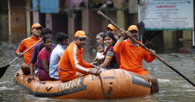
Situated along the eastern coast of India, Chennai is exposed to violent storm surges and flooding during northeast monsoons (September to November). Although local flooding is an annual phenomenon in selected parts of the city, extreme events, such as the 1918 cyclone and 1985 floods, had faded from people’s memory. [2]  However, history repeated itself in the city and neighboring coastal districts in November-December 2015, when a devastating flood affected more than 4 million people, claimed more than 470 lives and resulted in enormous economic loss. [3]

The sudden and unprecedented nature of the flood led to ad hoc and uncoordinated relief and response activities by different governmental and non-governmental agencies. Industrial and commercial centers were forced to temporarily shut down their production due to loss of power, shelter and limited logistics. Amid the chaos and widespread impact, the event brought people and institutions in and outside Chennai together, to provide support to the victims affected by the flood. Help reached the affected areas and their residents from different sections of society and in variety of forms. The lessons from this case study and others like it can help urban centers elsewhere in Asia to plan for similar eventualities.

Challenges Faced During and Following the Event

Flooding often handicaps the affected community by adversely affecting its educational system, food availability, mobility and access to energy on a daily basis. Chennai was no exception: daily functions became a challenge for the entire city.

School authorities faced numerous challenges, ranging from the sudden need to shift and secure school records / admit cards and postpone exams, to maintaining physical infrastructure and equipping schools to serve as shelters. Following the event, school authorities faced yet another set of daunting tasks related to the resumption of the academic session (e.g. repairing and replacing furniture, etc.) in schools that had been shuttered (for 10 to 33 days) in various parts of the city.

Flooding often handicaps the affected community by adversely affecting its educational system, food availability, mobility and access to energy on a daily basis.

Food logistics arrangements across the affected communities included the unavailability of manufacturing capacity and delivery mechanisms. The lack of accessibility to several parts of Chennai due to severe flooding made identification of delivery points and transport routes more difficult, which deprived some local communities of basic food supplies required for survival. During the first 24 hours of flooding, the main concern of the local supermarkets providing food supplies to surrounding areas, was to safeguard perishable items not only from getting wet but also to keep them from spoiling (since there was no electricity). However, it was critical for them to meet customer demand, keeping in mind the limited food availability and lack of communication within their management team.

First responders and information providers faced difficulties in providing accurate real time information to local communities on flooded areas, accessibility of roads, road condition, traffic flow and current weather scenario.

Flooding of roads, tracks and supporting infrastructure, delayed and suspended provision of necessary services. Moreover, several hospital staff were unable to get to work or extend their support due to being affected by the flood themselves. It was a greater challenge for hospital authorities, to safeguard patients admitted to Intensive and Critical Care units (ICU) or those under ventilation through maintenance of power supply.

The Chennai flood had a devastating impact on businesses, especially on small and medium-sized enterprises (SMEs), who were unprepared and vulnerable to both direct and indirect impacts. Flood water entered the first level of most of the offices and shops, reaching a height of approximately two meters in some areas. This damaged products, stocks, storage units, electrical equipment. In post disaster scenario, several businessmen in Chennai were unable to operate for three months due to lack of process-service delivery, finance, logistics, management implications and loss of customer base. Service station owners too had a hard time in recovering broken cars, fixing damaged engines, car interiors, upholsteries and external impact damages. In post flood scenario fungal attack and rusting were additional issues faced by them to continue their business.

Community-Based Organizations (CBOs) faced a plethora of challenges and obstacles, as did official first responders ...

Community-Based Organizations (CBOs) faced tough challenges, such as contingency planning at zone/ district level, stock piling of relief materials/supplies, arranging for inter-agency coordination, preparing evacuation plans, providing public information and conducting field exercises. Service providers in the transport sector had to undertake route planning and ensure priority management. Situation worsened due to lack of mechanisms to mitigate impacts of flood, such as road closure notification, absence of traffic control warning signs, emergency detour routes, etc. which are essential during such extreme events. Thus, they procured boats and hired fishermen to commute to inundated parts of the city.

Likewise, government officials — first responders, such as the fire department, the National Disaster Response Force (NDRF) and the police, in particular — faced a plethora of challenges and obstacles. They not only had the responsibility of conducting rescue operations, but also of road clearance and provision of other facilities to ensure supply of basic necessities throughout the affected communities. The fire department managed calls, coordinated between departments and controlled water distribution system, in the absence of power for prolonged periods. They had to function with disrupted utility services, clear streets of debris, waste and fallen trees in low lying areas and also ensure steady and quick pumping out of water from flooded pockets. NDRF on the other hand, was required to conduct timely rescue operations with small teams, coordinate with local officials, mobilize limited human resources to priority areas and commute using limited transport vehicles and boats. They also had electricity constraints in setting up onsite operational coordination control room (OSOCC) and shelters for both their team as well as the local community. In some instances, the Chennai police were unable to ensure effective and timely response, due to lack of common command system, clear assignment of duties and demarcation of roles to respective officials, for times of emergency.

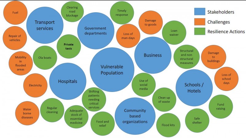
Resilience Efforts

Various segments of society assisted local communities and relief providers in affected parts of Chennai to cope with the flood. The Chennai government, private schools and the Parent Association were three strong pillars which supported victims in the aftermath of the flood. School children from Hosur made artefacts for sale at an art show to raise funds for a severely affected government school in Poonamallee. Another group of 15 teachers and 40 alumni of the TVS Academy School of Hosur, travelled to Chennai to help improve the infrastructure of Aringar Anna Government Girls Higher Secondary School, Poonamallee. These groups extended help in painting damaged walls, blackboards and building new toilets. During and post flood, government schools were used as relief camps where food and health issues were partially covered by government and parent association.

Various segments of society assisted local communities and relief providers in affected parts of Chennai to cope with the flood.

Private enterprises, such as restaurants, taxi service providers and automobile service centers, also joined hands with the government to provide relief to the flood affected population. Kolapasi, a Chennai-based restaurant, was turned into a temporary food relief agency. Social media was used for awareness generation on the initiative and also to raise funds. Individuals of all age groups and across all professions, supported this initiative by volunteering to cook, wash utensils, pack and deliver food. About 1.7 lakhs food boxes were distributed across the city.

The ride-hailing company Ola started operating boats, which also provided an important learning for future preparedness measures. They strategically identified water routes for providing service to even the most inaccessible areas. They also helped the Fire Department in conducting their rescue operations. Similarly, a vegetable and milk supply chain, Heritage Fresh, sold their commodities at a subsidized rate when prices in parts of Chennai were on the rise. Mobile vegetable shops also put in efforts to reach out to as many flood affected people as possible. Online food service providers, such as Zomato, added one extra meal on behalf of the company for every order that was placed for the stranded people.

The impact of flood on health sector was a complex issue, as the threats to health were both direct (for example, flash flood) and indirect (for example, a hospital needing to be closed due to flooding). To protect and promote health of patients and minimize health risks, sustained treatment for chronic infectious disease were provided through voluntary camps. 51 patients were evacuated and ICU wards were shifted to first floor; special care was taken while shifting new born babies, mental patients, elderly or patients with disabilities; cleanliness was ensured by internal experts using prescribed norms and dosage of chemicals and sump pumps were installed in hospitals to drain out water. Adequate stock of medicine, injections and IV fluids (intravenous) were available for continued medical care of the patients. Immediate actions in response to the flash flood situation from the ESIC was to direct all capacities of the existing health care system towards flood relief, prevention of disease outbreak, water disinfection and vigilance for future outbreaks.

Funds for energy and fuel supply were of least priority, but their demand was high in slums and remote areas where it was required for the survival of sick family members, the elderly and children. Organizations like Oxfam, provided support through the provision of energy and fuel supply to households. Private companies like Servals Pvt Ltd. initiated a similar program of providing specially designed rehabilitation kit, which included a kerosene stove, water filter, utensils, disinfectant, etc. to the slum dwellers, manual laborers and villagers in the worst hit areas, who were not covered under government programs. Along with the kit, training was also provided to ensure optimum utilization of the given products. 

Small- and medium-sized enterprises (SMEs) suffered both direct (physical) and indirect (man-days/ sales) loss. They demanded government to provide interest free loans and delay their tax payment along with other repayments. SMEs took adequate measures to build resilience against future floods through installation of electrical points at a raised height and flood defense barriers within their premises, securing databases by using online recovery systems, etc.

Vehicle service stations, such as Harsha Toyota collected and repaired cars that broke down due to water logging. Company ordered its dealerships to take extra space for flood affected cars while insurance companies were asked to clear their claims on time. They also provided discounted service packages, such as completely waiving labor charges, and offering ten percent discounts on spare parts, roadside assistance, loyalty points of up to Rs. 20,000, 50 percent discounts on car renewal and an exchange bonus up to Rs. 30,000 to flood-affected areas. The 2015 Chennai flash flood made all the car companies (e.g., Toyota, BMW, Renault, Maruti, Hyundai, Nissan, etc.) rethink and develop more sustainable business continuity plan for production, maintenance and parking. Several online and local sellers including a number of automobile portals, such as Copart, has a separate page exclusively for cars damaged in Chennai floods for holding auctions.

Hotel authority liaised with local authorities (i.e., police and fire service and incorporated emergency plans and services wherever possible. Guests were relocated and although flood kits (water proof clothing, blanket, candle/torches, etc.) was provided to all, there is a need to strengthen response and relief capacity of hotels.

Community-Based Organizations (CBOs), such as Tamil Nadu Thowheed Jamath (TNTJ) mobilized over 700 volunteers for carrying out rescue, relief, rehabilitation and reconstruction work, which included arranging food, shelter, cleaning up after flood water resided, waste management, spraying of insecticides and distribution of relief kit. They used half-cut plastic tank boats to rescue stranded people, conducted community based training programmes in health risks and fostered behavioral changes to support all social groups. TNTJ also became one of the coordinating facilitator through establishment of community, zone and district level mechanism with local partners, frontline workers and line departments.

Social media, such as Facebook, Twitter, and Google Maps, played an important role in bringing all the service providers and individuals to work together for reducing the impact and helping the flood affected population recover better. These platforms helped disseminate information, broadcast further warnings, inform people of the undertaken initiatives, call for volunteers in respective sectors, crowdsource and map the waterlogged or inundated areas. Professor Amit Sheth and his team at Wright State University in the United States carried out a new National Science Fund (NSF)-funded project, the Social and Physical Sensing Enabled Decision Support for Disaster Management and Response. This technology was mobilized  to monitor and analyze social media and crowdsourcing for better situational awareness of Chennai flood. Companies, such as BSNL, Paytm, Airtel and Zomato, also pitched in to help Chennai flood victims.

Towards Building Urban Disaster Risk Resilience

The 2015 Chennai flood caused by the torrential downpour brought city life to a standstill. It affected socio-economic condition of the district, maimed critical infrastructure, stranded animals and humans, disrupted services and flooded major parts of the city. The incorporation of flood preparedness measures will help reduce the extent of their impact on people, their life and property in future, along with giving them better coping abilities.

Best practices from Chennai flood case study should be used to strengthen existing risk handling capacities as well as learn lessons, to help replicate similar initiatives for preparedness of other Indian cities. This will also enable the government to coordinate and collaborate with similar service providers across the city for conducting efficient rescue and response operations in future. Best practices extrapolated from this case study could also prove useful to local and national officials from countries throughout Asia and the Middle East, all of whom continue to wrestle with the complex challenges associated with responding to responding to natural disasters in urban settings.    

Prioritized interventions and emergency responses which can be used to reduce urban risk, redevelop city plans and ensure effective disaster relief operations in future are listed below.

➢ As was reflected in the initiatives undertaken by several CBOS, particularly TNTJ, disaster response should address the humanitarian imperative; adhere to the principles of neutrality and impartiality; and ensure local participation and accountability, along with respecting local culture and custom. Thus, awareness generation and capacity building programs should promote inclusive flood disaster management approaches. Operational and sustainable livelihood models should be developed in the aftermath of such emergencies for weaker sections of the society. Disaster resistant shelters, public buildings and critical infrastructure, such as water and sewerage networks, need to be improved in order to avoid water logging and enhance community resilience.

➢ Cities need to develop broadcasting systems to inform the affected community about real time extreme events in different locales and provide updates on current road, flood, weather, food and energy supply scenario. Social media helps develop a two-way communication which helps acquire real time information from the community itself.

➢ Development of city disaster risk resilience strategy will better enable government and non-government organizations in phasing out adaptation and mitigation measures during normalcy.

➢ To ensure community level disaster preparedness, designed trainings should include actions or steps to be taken by citizen prior to, during and after disaster scenarios. Emergency respondents need to have basic first aid skills, such as airway management, bleeding control and simple triage.

➢ Emotional impact of the event on both workers as well as victims need to be addressed and documented for informing city disaster management plan.

➢ GIS-based evacuation plans, including current flood water flow, emergency routes, water depth, obstacles and possible search and rescue (SAR) interventions, need to be prepared. Existing capacity needs to be strengthened and assistance programmes should be provided to existing or new SAR teams at district and state level, for future preparedness. In addition, there is also a need to prepare Flood Risk Maps highlighting availability of grocery stores, restaurants, public utilities, food storage units, hospitals, residential homes for elderly people, high flood prone areas, etc.

➢ Communication systems, including early warning and public awareness mechanisms, need to be established in order to disseminate information during adverse conditions. (There is also an urgent need to prioritize child protection for the prevention of child trafficking during disasters.)

➢ Adaptation strategies need to ensure raised utility and reduced food cost through development and strengthening of local food suppliers. Food supply chain should be maintained by improved coordination and efficiency between producers, suppliers and retailers.

➢ Local flood plain maps, should inform construction practices (e.g., selection of appropriate materials for walls and floors).

➢ In flood-prone areas, water proofing should be mandated for emergency facilities like- power control room, water treatment plants, sewerage plants, etc. Emergency food and assets (generator sets, fuel) area should be at an elevated level to prevent inundation due to flooding.

Note: The detailed assessment of interventions undertaken during and post Chennai floods was funded by Rockefeller Foundation under the Asian Cities Climate Change Resilience Network program. The study was conducted by Taru Leading Edge and IFMR Chennai.

[1] “Chennai Metropolitan Urban Region Population 2011 Census,” accessed May 29, 2017, http://www.census2011.co.in/census/metropolitan/435-chennai.html .

[2] Deepa H. Ramakrishnan, “Memories of Rain Ravaged Madras,” The Hindu, December 9, 2015, accessed May 29, 2017, http://www.thehindu.com/news/cities/chennai/floods-in-madras-over-years… .

[3] “Letter from Chennai- Saving a home from floods,” The National, January 17, 2015, accessed May 29, 2017, http://www.thenational.ae/world/south-asia/20151213/letter-fromchennai-saving-a-home-from-the-floods ; “When Chennai was logged out and how,” Deccan Chronicle, accessed March 29, 2017; and http://www.deccanchronicle.com/151203/nation-currentaffairs/article/when-chennai- was-logged-out-and-how.B. Narasimhan, “Storm water drainage of Chennai: Lacuna, Assets, and Way Forward.” Presentation made at “Resilient Chennai: Summit on Urban Flooding,” hosted by 100 Resilient Cities in partnership with the Corporation of Chennai (2016). 

The Middle East Institute (MEI) is an independent, non-partisan, non-for-profit, educational organization. It does not engage in advocacy and its scholars’ opinions are their own. MEI welcomes financial donations, but retains sole editorial control over its work and its publications reflect only the authors’ views. For a listing of MEI donors, please click here .

• 2023 Lancet Countdown U.S. Launch Event
• 2023 Lancet Countdown U.S. Brief
• PAST BRIEFS

2020 CASE STUDY 2

The 2019 floods in the central u.s..

Lessons for Improving Health, Health Equity, and Resiliency

In spring 2019, the Midwest region endured historic flooding that caused widespread damage to millions of acres of farmland, killing livestock, inundating cities, and destroying infrastructure. CS_52

The Missouri River and North Central Flood resulted in over $10.9 billion of economic loss in the region, making it the costliest inland flood event in U.S. history. CS_52 Yet, this is just the beginning, as climate change continues to accelerate extreme precipitation, increasing the likelihood of severe events previously thought of as “once in 100 year floods.” CS_53 , CS_54

This 2019 disaster exhibited the same health harms and healthcare system disruptions seen in previous flooding events, and vulnerable populations – notably tribal and Indigenous communities – were once again disproportionately impacted. Thus, there is an enormous need for policy interventions to minimize health harms, improve health equity, and ensure community resilience as the frequency of these weather events increases.

Before-and-after images of catastrophic flooding in Nebraska. Left image taken March 20, 2018. Right image taken March 16, 2019.

Source: NASA Goddard Space Flight Center, with permission

The role of climate change, widespread devastation, and compounding inequities

The Missouri River and North Central Flood were the result of a powerful storm that occurred near the end of the wettest 12-month period on record in the U.S. (May 2018 – May 2019). CS_55 , CS_56 The storm struck numerous states, specifically Nebraska (see Figure 1), Iowa, Missouri, South Dakota, North Dakota, Minnesota, Wisconsin, and Michigan. Two additional severe flooding events occurred in 2019 in states further south, involving the Mississippi and Arkansas Rivers.

This flood event exhibits two key phenomena that have been observed over the last 50 years as a result of climate change: annual rainfall rates and extreme precipitation have increased across the country. CS_57 The greatest increases have been seen in the Midwest and Northeast, and these trends are expected to continue over the next century. Future climate projections also indicate that winter precipitation will increase over this region, CS_57 further increasing the likelihood of more frequent and more severe floods. For example, by mid-century the intensity of extreme precipitation events could increase by 40% across southern Wisconsin. CS_58 While it is too early to have detection and attribution studies for these floods, climate change has been linked to previous extreme precipitation and flood events. CS_59 , CS_60

Hundreds of people were displaced from their homes and millions of acres of agricultural land were inundated with floodwaters, killing thousands of livestock and preventing crop planting. CS_52 , CS_61 , CS_62 Federal Emergency Management Agency (FEMA) disaster declarations were made throughout the region, allowing individuals to apply for financial and housing assistance, though remaining at the same housing site continues to place them at risk of future flood events.

In Nebraska alone, 104 cities, 81 counties and 5 tribal nations received state or federal disaster declarations. FEMA approved over 3,000 individual assistance applications in Nebraska, with more than $27 million approved in FEMA Individual and Household Program dollars. In addition to personal property, infrastructure was heavily affected, with multiple bridges, dams, levees, and roads sustaining major damage (see Figure 2). CS_52

Destruction of Spencer Dam during Missouri River and North Central Floods. CS_63

• Oglala Sioux Tribe, Cheyenne River Sioux Tribe of the Cheyenne River Reservation, Standing Rock Sioux Tribe (North Dakota and South Dakota), Yankton Sioux Tribe of South Dakota, Lower Brule Sioux Tribe of the Lower Brule Reservation, Crow Creek Sioux Tribe of Crow Creek Reservation, Sisseton-Wahpeton Oyate of the Lake Traverse Reservation, Rosebud Sioux Tribe of the Rosebud Sioux Indian Reservation, Santee Sioux Nation, Omaha Tribe of Nebraska, Winnebago Tribe of Nebraska, Ponca Tribe of Nebraska, Sac & Fox Nation of Missouri (Kansas and Nebraska), Iowa Tribe of Kansas and Nebraska, and Sac & Fox Tribe of the Mississippi in Iowa.

Source: Nebraska Department of Natural Resources, with permission.

As with other climate-related disasters, the 2019 floods had devastating effects on already vulnerable communities as numerous tribes and Indigenous peoples were impacted,° adding to centuries of historical trauma. CS_64 , CS_65 Accounts of flooding on the Pine Ridge Reservation in South Dakota demonstrate the challenges that resource-limited communities face in coping with extreme weather events. CS_64 Delayed response by outside emergency services left tribal volunteers struggling to help residents stranded across large distances without access to supplies, drinking water, or medical care.66 Lack of equipment and limited transportation hampered evacuations. CS_67

Health harms and healthcare disruptions

There were three recorded deaths from drowning, but hidden health impacts were widespread and extended well beyond the immediate risks and injuries from floodwaters. In the aftermath, individuals in flooded areas were exposed to hazards like chemicals, electrical shocks, and debris. CS_68 Water, an essential foundation for health, was contaminated as towns’ wells and other drinking water sources were compromised. This put people, especially children, at increased risk for health harms like gastrointestinal illnesses. CS_69 Stranded residents relied on shipments of water from emergency services and volunteer organizations and the kindness of strangers ( see Box 1 ).

BOX 1: “We just remember the trust and commitment to each other”

Linda Emanuel, a registered nurse and farmer living in the hard-hit rural area of North Bend in Nebraska, helped organize flood recovery efforts. She recalled wondering, “How are we going to handle this? How do we inform the people of all the hazards without scaring them?” In addition to her educational role, she administered a limited supply of tetanus shots, obtained and distributed hard-to-find water testing kits, and coordinated PPE usage. In the first days of the flooding, she hosted some 25 stranded individuals in her home. Reminiscing about how community members came together amidst the devastation, Emanuel remarked, “We just remember the trust and the commitment to each other and to our town. We are definitely a resilient city.” CS_70

Standing water remained in many small town for months, and a four-year old child at the Yankton Sioux reservation in South Dakota likely contracted Methicillin-resistant Staphylococcus aureus (MRSA) after playing in a pond. CS_71 The mold and allergens that developed in the aftermath of the floods exacerbated respiratory illness. CS_72 Flooding also backed up sewer systems into basements; clean up required personal protective equipment (PPE) to prevent the potential spread of infectious diseases. The significant financial burdens, notably the loss of property in the absence of adequate insurance, can contribute to serious mental and emotional distress in flood victims. CS_73 , CS_74

Infrastructure disruptions, like flooded roads, meant that many individuals in rural areas were unable to access essential services including healthcare. In an interview with the New York Times, Ella Red Cloud-Yellow Horse, 59, from Pine Ridge Indian Reservation, recounts her own struggle to get to the hospital for a chemotherapy appointment. CS_64 After being stranded by flooding for days, she had contracted pneumonia, but she couldn’t be reached by an ambulance or tractor because her driveway was blocked by huge amounts of mud. She was forced to trudge through muddy flood waters for over an hour to get to the highway.

She told the Times, “I couldn’t breathe, but I knew I needed to get to the hospital.” Her story is an increasingly common occurrence as critical infrastructure is damaged by climate change-intensified extreme events. These infrastructure challenges are also often superimposed on top of the challenges of poverty and disproportionate rates of chronic diseases ( see the Case Study ). Multiple hospitals sustained damage and several long-term care facilities were forced to evacuate, with some closing permanently, as a result of the rising floodwaters, CS_75 likely exacerbating existing diseases.

A path towards a healthier, equitable, and more resilient future

As human-caused climate change increases the likelihood of precipitation events that can cause severe flooding disasters, public health systems must serve as a first line of defense against the resulting health harms. As such, the broader public health system needs to develop the capacity and capability to understand and address the health hazards associated with climate-related disasters. Often funds and resources for these efforts are focused on coastal communities; however, inland states face many climate-related hazards that are regularly overlooked. Building on or expanding programs similar to CDC’s Climate-Ready States and Cities Initiative will help communities in inland states prepare for future climate threats. CS_76

Additionally, public health officials, health systems, and climate scientists should collaborate to create robust early warning systems to help individuals and communities prepare for flood events. Education regarding the health impacts of flooding should not be limited to the communities affected, but it should also include policymakers and other stakeholders who can implement systemic changes to decrease and mitigate the effects of floods. Local knowledge offered by community members regarding water systems, weather patterns, and infrastructure will be essential for effective and context-specific adaptation. By implementing these changes and executing more inclusive flood emergency plans, communities will be better situated to face the flood events that are projected to increase in the years to come.

Introduction – Figure 1: Nebraska Flooding The Role of Climate Change – Figure 2: Destruction of Spencer Dam Health Harms and Healthcare Disruptions – Box 1: Remember the Trust A Path Towards Equality

Advertisement

Analysis of flood damage and influencing factors in urban catchments: case studies in Manila, Philippines, and Jakarta, Indonesia

• Original Paper
• Published: 10 September 2020
• Volume 104 , pages 2461–2487, ( 2020 )

Cite this article

• Mohamed Kefi 1 , 5 ,
• Binaya Kumar Mishra 2 , 5 ,
• Yoshifumi Masago 3 , 5 &
• Kensuke Fukushi 4 , 5  

2159 Accesses

9 Citations

Explore all metrics

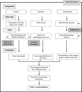
The sustainability and efficiency of flood risk management depends on the assessment of flood hazards and on the quantification of flood damage. Under the conditions of climate change and rapid urbanization, the evaluation of flood risk can lead to the success of adaptation strategies. The main objectives of this study are the estimation of future direct flood damage in two urban watersheds: The Pasig–Marikina–San Juan River in Metro Manila, Philippines, and the Ciliwung River in Jakarta, Indonesia, as well as the determination of the relation between factors that drive floods and flood damage. A spatial analysis approach based on the integration of several parameters, such as flood hazard, climate, and property value, was applied using a Geographic Information System (GIS). The flood depth-damage function generated from the field surveys was employed for the analysis to identify the spatial distribution of flood loss. The findings showed that, under future scenarios (target year: 2030), the total flood damage will increase by 212% and 80% in the target areas of Manila and Jakarta, respectively, compared to the current scenarios. This growth is due to the higher level of extreme rainfall events and to the degree of urbanization in the future. A comparative analysis of the two study areas highlighted the significant effects of the level of water depth and the inundated areas on flood damage, depending on the sites. This study is useful for local decision makers to implement suitable strategies for urban planning and flood control.

This is a preview of subscription content, log in via an institution to check access.

Access this article

Price includes VAT (Russian Federation)

Instant access to the full article PDF.

Rent this article via DeepDyve

Institutional subscriptions

Similar content being viewed by others

Flooding trends and their impacts on coastal communities of Western Cape Province, South Africa

Integrated monitoring and modeling to disentangle the complex spatio-temporal dynamics of urbanized streams under drought stress

GIS-based flood risk assessment using multi-criteria decision analysis of Shebelle River Basin in southern Somalia

Data availability.

The data collected and used in this study are strictly anonymous and are used for research purposes only.

ADB (Asian Development Bank) (2013) The rise of natural disasters in Asia and the Pacific: learning from ADB’s experience. Independent Evaluation at ADB. ADB (Asian Development Bank), Mandaluyong

Google Scholar  

ADB (Asian Development Bank) (2015) Global increase in climate-related disasters, working paper November 2015. Independent evaluation at ADB. ADB (Asian Development Bank), Metro Manila

Afifi Z, Chu HJ, Kuo YL, Hsu YC, Wong HK, Zeeshan Ali M (2019) Residential flood loss assessment and risk mapping from high-resolution simulation. Water 11:751. https://doi.org/10.3390/w11040751

Article   Google Scholar  

Albano R, Mancusi L, Sole A, Adamowski J (2015) Collaborative strategies for sustainable EU flood risk management: FOSS and geospatial tools—challenges and opportunities for operative risk analysis. ISPRS Int J Geo-Inf 4:2704–2727. https://doi.org/10.3390/ijgi4042704

Asdak C, Supian S, Subiyanto (2018) Watershed management strategies for flood mitigation: a case study of Jakarta’s flooding. Weather Clim Extrem 21:117–122. https://doi.org/10.1016/j.wace.2018.08.002

Bathrellos GD, Karymbalis E, Skilodimou HD, Gaki-Papanastassiou K, Baltas EA (2016) Urban flood hazard assessment in the basin of Athens Metropolitan city, Greece. Environ Earth Sci 75:319. https://doi.org/10.1007/s12665-015-5157-1

Campbell JB (2007) Introduction to remote sensing, 4th edn. The Guilford press, New York

Centre for Research on the Epidemiology of Disasters (2018) EM-DAT: the emergency events database. https://www.emdat.be . Accessed 03 May 2018

Chiba Y, Shaw R, Prabhakar S (2017) Climate change related non-economic loss and damage in Bangladesh and Japan. Int J Clim Change Strateg 9(2):166–183. https://doi.org/10.1108/IJCCSM-05-2016-0065

CTI Engineering International Co., Ltd and WCI, Woodfields Consultants, Inc. (2013) Master plan for flood management in Metro Manila and surrounding areas. Department of Public Works and Highways, the World Bank and AusAID, Tokyo

Dang NM, Babel MS, Luong HT (2011) Evaluation of flood risk parameters in the day river flood diversion area, Red River Delta, Vietnam. Nat Hazards 56(1):169–194. https://doi.org/10.1007/s11069-010-9558-x

De Moel H, Aerts JCJH (2011) Effect of uncertainty in land use, damage models and inundation depth on flood damage estimates. Nat Hazards 58(1):407–425. https://doi.org/10.1007/s11069-010-9675-6

Dutta D, Herath S, Musiake K (2003) A mathematic model for loss estimation. J Hydrol 227(1–2):24–49. https://doi.org/10.1016/S0022-1694(03)00084-2

Dutta D, Wright W, Rayment P (2011) Synthetic impact response functions for flood vulnerability analysis and adaptation measures in coastal zones under changing climatic conditions: a case study in Gippsland coastal region, Australia. Nat Hazards 59(2):967–986. https://doi.org/10.1007/s11069-011-9812-x

Fankhauser S, Dietz S, Gradwell P (2014) Non-economic losses in the context of the UNFCCC work programme on loss and damage (policy paper). Centre for Climate Change Economics and Policy, Grantham Research Institute on Climate Change and the Environment, London

Feldman AD (2000) Hydrologic modeling system HEC-HMS technical reference manual, U.S. Army Corps of Engineers, Hydrologic Engineering Center, HEC Davis, CA, USA

Fohrer N, Haverkamp S, Eckhardt K, Frede HG (2001) Hydrologic response to land use changes on the catchment scale. Phys Chem Earth Part B Hydrol Oceans Atmos 26(7–8):577–582. https://doi.org/10.1016/S1464-1909(01)00052-1

Foudi S, Oses-Eraso N, Tamayo I (2015) Integrated spatial flood risk assessment: the case of Zaragoza. Land Use Policy 42:278–292. https://doi.org/10.1016/j.landusepol.2014.08.002

Glas H, Jonckheere M, Mandal A, James-Williamson S, De Maeyer P, Deruyter G (2017) A GIS-based tool for flood damage assessment and delineation of a methodology for future risk assessment: case study for Annotto Bay, Jamaica. Nat Hazards 88:1867–1891. https://doi.org/10.1007/s11069-017-2920-5

Guha-Sapir D, Hoyois Ph, Wallemacq P, Below R (2016) Annual disaster statistical review 2016, the numbers and trends. CRED, Brussels

Handmer J (2002) The chimera of precision: inherent uncertainties in disaster loss assessment. Int J Mass Emerg Disaster 20(2):325–346

Huizinga J, De Moel H, Szewczyk W (2017). Global flood depth-damage functions. Methodology and the database with guidelines. EUR 28552 EN. https://doi.org/10.2760/16510

IPCC (Intergovernmental Panel on Climate Change) (2012) Managing the risks of extreme events and disasters to advance climate change adaptation. In: Field CBV, Barros TF, Stocker D, Qin DJ, Dokken KL, Ebi MD, Mastrandrea KJ, Mach GK, Plattner SK, Allen M et al (eds) A special report of Working Groups I and II of the Intergovernmental Panel on Climate Change. Cambridge University Press, Cambridge

Jalilov SM, Kefi M, Kumar P, Masago Y, Mishra BK (2018) Sustainable urban water management: application for integrated assessment in Southeast Asia. Sustainability 10(1):122. https://doi.org/10.3390/su10010122

Jongman B, Kreibich H, Barredo JI, Bates PD, Feyen L, Gericke A, Neal J, Aerts JCJH, Ward PJ (2012) Comparative flood damage model assessment: towards a European approach. Nat Hazard Earth Syst 12:3733–3752. https://doi.org/10.5194/nhess-12-3733-2012

Jonkman SN, Bockarjova M, Kok M, Bernardini P (2008) Integrated hydrodynamic and economic modelling of flood damage in the Netherlands. Ecol Econ 66(1):77–90. https://doi.org/10.1016/j.ecolecon.2007.12.022

Kefi M, Mishra BK, Kumar P, Masago Y, Fukushi K (2018) Assessment of tangible direct flood damage using a spatial analysis approach under the effects of climate change: case study in an urban watershed in Hanoi, Vietnam. ISPRS Int J Geo-Inf 7(1):29. https://doi.org/10.3390/ijgi7010029

Komolafe AA, Herath S, Avtar R (2015) Sensitivity of flood damage estimation to spatial resolution. J Flood Risk Manag. https://doi.org/10.1111/jfr3.12224

Komolafe AA, Herath S, Avtar R (2018) Development of generalized loss functions for rapid estimation of flood damages: a case study in Kelani River basin, Sri Lanka. Appl Geom 10(1):13–30. https://doi.org/10.1007/s12518-017-0200-4

Komori D, Nakamura S, Kiguchi M, Nishijima A, Yamazaki D, Suzuki S, Kawasaki A, Oki K, Oki T (2012) Characteristics of the 2011 Chao Phraya River flood in Central Thailand. Hydrol Res Lett 6:41–46. https://doi.org/10.3178/hrl.6.41

Kreibich H, Thieken AH (2008) Assessment of damage caused by high groundwater inundation. Water Resour Res 44:W09409. https://doi.org/10.1029/2007WR006621

Kundzewicz ZW, Kanae S, Seneviratne SI, Handmer J, Nicholls N, Peduzzi P, Mechler R, Bouwer LM, Arnell N, Mach K, Muir-Wood R, Brakenridge GR, Kron W, Benito G, Honda Y, Takahashi K, Sherstyukov B (2014) Flood risk and climate change: global and regional perspectives. Hydrol Sci J 59(1):1–28. https://doi.org/10.1080/02626667.2013.857411

Lagmay AM, Mendoza J, Cipriano F, Delmendo PA, Lacsamana MN, Moises MA, Pellejera NIII, Punay KN, Sabio G, Santos L, Serrano J, Taniza HJ, Tingin NE (2017) Street floods in Metro Manila and possible solutions. J Environ Sci 59:39–47. https://doi.org/10.1016/j.jes.2017.03.004

Lechowska E (2018) What determines flood risk perception? A review of factors of flood risk perception and relations between its basic elements. Nat Hazards 94:1341–1366. https://doi.org/10.1007/s11069-018-3480-z

Mall RK, Srivastava RK (2012) Sustainable flood management in changing climate. Mishra OP, Ghatak M, Kamal A (eds) SAARC workshop on flood risk management in South Asia FLOOD, 9–10 October 2012, Islamabad, Pakistan. Published by the SAARC Disaster Management Centre, New Delhi

Mardiah ANR, Lovett JC, Evanty N (2017) Toward integrated and inclusive disaster risk reduction in Indonesia: review of regulatory frameworks and institutional networks. In: Djalante R, Garschagen M, Thomalla F, Shaw R (eds) Disaster risk reduction in Indonesia: progress, challenges, and issues. Springer, Berlin

Merz B, Kreibich H, Schwarze R, Thieken A (2010) Assessment of economic flood damage. Nat Hazard Earth Syst 10:1697–1724. https://doi.org/10.5194/nhess-10-1697-2010

Messner F, Penning Rowsell E, Green C, Meyer V, Tunstall S, Vander Veen A (2007) Evaluating flood damages : guidance and recommendations on principles and methods; FLOOD site integrated flood risk analysis and management methodologies report T09-06-01; HR Wallingford: Oxfordshire, UK

Mishra B, Herath S (2011) Climate projections downscaling and impact assessment on precipitation over upper Bagmati River Basin. In: Proceedings of third international conference on addressing climate change for sustainable development through up-scaling renewable energy technologies. Tribhuvan University, Kathmandu, Nepal, 2011, pp 275–281

Mishra BK, Rafiei Emam A, Masago Y, Kumar P, Regmi RK, Fukushi K (2017) Assessment of future flood inundations under climate and land use change scenarios in the Ciliwung River Basin. J Flood Risk Manag, Jakarta. https://doi.org/10.1111/jfr3.12311

Book   Google Scholar  

Moss RH, Edmonds JA, Hibbard KA, Manning MR, Rose SK, Van Vuuren DP, Carter TR, Emori S, Kainuma M, Kram T, Meehl GA, Mitchell JF, Nakicenovic N, Riahi K, Smith SJ, Stouffer RJ, Thomson AM, Weyant JP, Wilbanks TJ (2010) The next generation of scenarios for climate change research and assessment. Nature 463(7282):747–756. https://doi.org/10.1038/nature08823

Nash JE, Sutcliffe JV (1970) River flow forecasting through conceptual models, part I: a discussion of principles. J Hydrol 10:282–290. https://doi.org/10.1016/0022-1694(70)90255-6

Neal JC, Bates PD, Fewtrell TJ, Hunter NM, Wilson MD, Horritt MS (2009) Distributed whole city water level measurements from the Carlisle 2005 urban flood event and comparison with hydraulic model simulations. J Hydrol 368:42–55. https://doi.org/10.1016/j.jhydrol.2009.01.026

Pathirage C, Seneviratne K, Amaratunga D, Haigh R (2014) Knowledge factors and associated challenges for successful disaster knowledge sharing. Input paper Prepared for the global assessment report on disaster risk reduction 2015. The United Nations Office for Disaster Risk Reduction (UNISDR), Global Assessment Report on Disaster Risk Reduction (GAR)

Pistrika A, Tsakiris G, Nalbantis I (2014) Flood depth-damage functions for built environment. Environ Process 1(4):553–572. https://doi.org/10.1007/s40710-014-0038-2

PSA (Philippine Statistics Authority) (2010) Census of population and housing Philippines, 2010. https://psa.gov.ph/sites/default/files/attachments/hsd/article/Table%201_2.pdf . Accessed 03 May 2018

PSA (Philippine Statistics Authority) (2015) Census of population. Republic of the Philippines, 2015. Accessed 03 May 2018

Rafiei Emam A, Mishra BK, Kumar P, Masago Y, Fukushi K (2016) Impact assessment of climate and land-use changes on flooding behavior in the Upper Ciliwung River, Jakarta, Indonesia. Water 8(12):559. https://doi.org/10.3390/w8120559

Richards JA, Jia X (2006) Remote sensing digital image analysis. An introduction fourth edition. Springer, Berlin

Serdeczny OM, Bauer S, Huq S (2018) Non-economic losses from climate change: opportunities for policy-oriented research. Climate Dev 10(2):97–101. https://doi.org/10.1080/17565529.2017.1372268

Smith DI (1994) Flood damage estimation—a review of urban stage-damage curves and loss functions. Water SA 20:231–238

Srinivasa Raju K, Nagesh Kumar D (2018) Impact of climate change on water resources with modeling techniques and case studies. Springer, Singapore

Stabinsky D, Singh H, Vaughan K, Champling R, Phillips J (2012) Tackling the limits to adaptation: an international framework to address “loss and damage” from climate change impacts. ActionAid. CARE International and WWF, Geneva

Te Linde AH, Bubeck P, Dekkers JEC, De Moel H, Aerts JCJH (2011) Future flood risk estimates along the river Rhine. Nat Hazard Earth Syst 11:459–473. https://doi.org/10.5194/nhess-11-459-2011

Thieken AH, Muller M, Kreibich H, Merz B (2005) Flood damage and influencing factors: new insights from the August 2002 flood in Germany. Water Resour Res 41:W12430. https://doi.org/10.1029/2005WR004177

UNDESA (United Nations, Department of Economic and Social Affairs) (2015) Population division world urbanization prospects: the 2014 revision (ST/ESA/SER.A/366)

Win S, Zin W, Kawasaki W, San Z (2018) Establishment of flood damage function MODELS: a case study in the Bago River Basin, Myanmar. Int J Disast Risk Reduct 28:688–700. https://doi.org/10.1016/j.ijdrr.2018.01.030

Zischg AP, Hofer P, Mosimann M, Röthlisberger V, Ramirez JA, Keiler M, Weingartner R (2018) Flood risk (d)evolution: disentangling key drivers of flood risk change with a retro-model experiment. Sci Total Environ 639:195–207. https://doi.org/10.1016/j.scitotenv.2018.05.056

Download references

Acknowledgements

The authors are grateful to the staff of Center of Environmental Research, Research and Community Services Institute, Bogor Agricultural University, Indonesia (PPLH –IPB), and local residents and local NGO in Metro Manila, Philippines, for their cooperation during the field survey.

This research was supported by the Japan Society for the Promotion of Science as Overseas researcher under Postdoctoral Fellowship of JSPS (Fellowship P16790). This work was also supported by the Water and Urban Initiative project of the United Nations University Institute for the Advanced Study of Sustainability (UNU-IAS), Tokyo, Japan.

Author information

Authors and affiliations.

Laboratory of Desalination and Natural Water Valorisation, Water Research and Technologies Center CERTE-Technopark of Borj Cedria, BP 273, 8020, Soliman, Tunisia

Mohamed Kefi

School of Engineering, Faculty of Science and Technology, Pokhara University, Pokhara-30, Kaski, Nepal

Binaya Kumar Mishra

Center for Climate Change Adaptation, National Institute for Environmental Studies, Tsukuba, Ibaraki, 305-8506, Japan

Yoshifumi Masago

Institute for Future Initiatives, The University of Tokyo, 7-3-1 Hongo, Bunkyo-ku, Tokyo, 113-0033, Japan

Kensuke Fukushi

United Nations University Institute for the Advanced Study of Sustainability, 5-53-70 Jingumae, Shibuya-ku, Tokyo, 150-8925, Japan

Mohamed Kefi, Binaya Kumar Mishra, Yoshifumi Masago & Kensuke Fukushi

You can also search for this author in PubMed   Google Scholar

Corresponding author

Correspondence to Mohamed Kefi .

Ethics declarations

Conflict of interest.

The authors declare that they have no conflict of interest.

Additional information

Publisher's note.

Springer Nature remains neutral with regard to jurisdictional claims in published maps and institutional affiliations.

Electronic supplementary material

Below is the link to the electronic supplementary material.

Questionnaire about flood event in Jakarta

Rights and permissions.

Reprints and permissions

About this article

Kefi, M., Mishra, B.K., Masago, Y. et al. Analysis of flood damage and influencing factors in urban catchments: case studies in Manila, Philippines, and Jakarta, Indonesia. Nat Hazards 104 , 2461–2487 (2020). https://doi.org/10.1007/s11069-020-04281-5

Download citation

Received : 18 January 2020

Accepted : 29 August 2020

Published : 10 September 2020

Issue Date : December 2020

DOI : https://doi.org/10.1007/s11069-020-04281-5

Share this article

Anyone you share the following link with will be able to read this content:

Sorry, a shareable link is not currently available for this article.

Provided by the Springer Nature SharedIt content-sharing initiative

• Flood damage
• Flood depth-damage function
• Climate change
• Urbanization
• Find a journal
• Publish with us
• Track your research

Can coastal cities turn the tide on rising flood risk?

Climate change is increasing the destructive power of flooding from extreme rain and rising seas and rivers. Many cities around the world are exposed. Strong winds during storms and hurricanes can drive coastal flooding through storm surge. As hurricanes and storms become more severe, surge height increases. Changing hurricane paths may shift risk to new areas. Sea-level rise amplifies storm surge and brings in additional chronic threats of tidal flooding. Pluvial and riverine flooding becomes more severe with increases in heavy precipitation. Floods of different types can combine to create more severe events known as compound flooding. With warming of 1.5 degrees Celsius , 11 percent of the global land area is projected to experience a significant increase in flooding, while warming of 2.0 degrees almost doubles the area at risk.

When cities flood, in addition to often devastating human costs, real estate is destroyed, infrastructure systems fail, and entire populations can be left without critical services such as power, transportation, and communications. In this case study we simulate floods at the most granular level (up to two-by-two-meter resolution) and explore how flood risk may evolve for Ho Chi Minh City (HCMC) and Bristol (See sidebar, “An overview of the case study analysis”). Our aim is to illustrate the changing extent of flooding, the landscape of human exposure, and the magnitude of societal and economic impacts.

An overview of the case study analysis

In Climate risk and response: Physical hazards and socioeconomic impacts , we measured the impact of climate change by the extent to which it could affect human beings, human-made physical assets, and the natural world. We explored risks today and over the next three decades and examined specific cases to understand the mechanisms through which climate change leads to increased socioeconomic risk.

In order to link physical climate risk to socioeconomic impact, we investigated cases that illustrated exposure to climate change extremes and proximity to physical thresholds. These cover a range of sectors and geographies and provide the basis of a “micro-to-macro” approach that is a characteristic of McKinsey Global Institute research. To inform our selection of cases, we considered over 30 potential combinations of climate hazards, sectors, and geographies based on a review of the literature and expert interviews on the potential direct impacts of physical climate hazards. We found these hazards affect five different key socioeconomic systems: livability and workability, food systems, physical assets, infrastructure services, and natural capital.

We ultimately chose nine cases to reflect these systems and to represent leading-edge examples of climate change risk. Each case is specific to a geography and an exposed system, and thus is not representative of an “average” environment or level of risk across the world. Our cases show that the direct risk from climate hazards is determined by the severity of the hazard and its likelihood, the exposure of various “stocks” of capital (people, physical capital, and natural capital) to these hazards, and the resilience of these stocks to the hazards (for example, the ability of physical assets to withstand flooding). We typically define the climate state today as the average conditions between 1998 and 2017, in 2030 as the average between 2021 and 2040, and in 2050 between 2041 and 2060. Through our case studies, we also assess the knock-on effects that could occur, for example to downstream sectors or consumers. We primarily rely on past examples and empirical estimates for this assessment of knock-on effects, which is likely not exhaustive given the complexities associated with socioeconomic systems. Through this “micro” approach, we offer decision makers a methodology by which to assess direct physical climate risk, its characteristics, and its potential knock-on impacts.

Climate science makes extensive use of scenarios ranging from lower (Representative Concentration Pathway 2.6) to higher (RCP 8.5) CO 2 concentrations. We have chosen to focus on RCP 8.5, because the higher-emission scenario it portrays enables us to assess physical risk in the absence of further decarbonization. (We also choose a sea-level rise scenario for one of our cases that is consistent with the RCP 8.5 trajectory). Such an "inherent risk" assessment allows us to understand the magnitude of the challenge and highlight the case for action. For a detailed description of the reason for this choice see the technical appendix of the full report.

Our case studies cover each of the five systems we assess to be directly affected by physical climate risk, across geographies and sectors. While climate change will have an economic impact across many sectors, our cases highlight the impact on construction, agriculture, finance, fishing, tourism, manufacturing, real estate, and a range of infrastructure-based sectors. The cases include the following:

• For livability and workability, we look at the risk of exposure to extreme heat and humidity in India and what that could mean for that country’s urban population and outdoor-based sectors, as well as at the changing Mediterranean climate and how that could affect sectors such as wine and tourism.
• For food systems, we focus on the likelihood of a multiple-breadbasket failure affecting wheat, corn, rice, and soy, as well as, specifically in Africa, the impact on wheat and coffee production in Ethiopia and cotton and corn production in Mozambique.
• For physical assets, we look at the potential impact of storm surge and tidal flooding on Florida real estate and the extent to which global supply chains, including for semiconductors and rare earths, could be vulnerable to the changing climate.
• For infrastructure services, we examine 17 types of infrastructure assets, including the potential impact on coastal cities such as Bristol in England and Ho Chi Minh City in Vietnam.
• Finally, for natural capital, we examine the potential impacts of glacial melt and runoff in the Hindu Kush region of the Himalayas; what ocean warming and acidification could mean for global fishing and the people whose livelihoods depend on it; as well as potential disturbance to forests, which cover nearly one-third of the world’s land and are key to the way of life for 2.4 billion people.

We chose these cities for the contrasting perspectives they offer: Ho Chi Minh City in an emerging economy, Bristol in a mature economy; Ho Chi Minh City in a regular flood area, Bristol in an area developing a significant flood risk for the first time in a generation.

We find the metropolis of Ho Chi Minh City can survive its flood risk today, but its plans for rapid infrastructure  expansion and continued economic growth could be incompatible with an increase in risk. The city has a wide range of adaptation options at its disposal but no silver bullet.

In the much smaller city of Bristol, we find a risk of flood damages growing from the millions to the billions, driven by high levels of exposure. The city has fewer adaptation options at its disposal, and its biggest challenge may be building political and financial support for change.

How significant are the flood risks facing Ho Chi Minh City and what can the city do?

Flooding is a common part of life in Ho Chi Minh City. This includes flooding from monsoonal rains, which account for about 90 percent of annual rainfall, tidal floods and storm surge from typhoons and other weather events. Of the city’s 322 communes and wards, about half have a history of regular flooding with 40 to 45 percent of land in the city less than one meter above sea level.

In our analysis, we quantify the possible impact on the city as floods hit real estate and infrastructure assets. 1 Flood modeling and expert guidance were provided by an academic consortium of Institute for Environmental Studies, Vrije Universiteit Amsterdam, and Center of Water Management and Climate Change, Vietnam National University. Infrastructure assets covered include both those currently available and those under construction, planned, or speculated. Knock-on effects are adjusted for estimates of economic and population growth. We simulate possible 1 percent probability flooding scenarios for the city for three periods: today, 2050, and a longer-term scenario of 180 centimeters of sea-level rise, which some infrastructure assets built by 2050 may experience as a worse-case in their lifetime (Exhibit 1).

• Today: We estimate that 23 percent of the city could flood, and a range of existing assets would be taken offline; infrastructure damage may total $200 million to $300 million. Knock-on effects would be significant, and we estimate could total a further $100 million to $400 million. Real estate damage may total $1.5 billion.
• 2050: A flood with the same probability in 30 years’ time would likely do three times the physical damage and deliver 20 times the knock-on effects. We estimate that 36 percent of the city becomes flooded. In addition, many of the 200 new infrastructure assets are planned to be built in flooded areas. As a result, the damage bill would grow, totaling $500 million to $1 billion. Increased economic reliance on assets would amplify knock-on effects, leading to an estimated $1.5 billion to $8.5 billion in losses. An additional $8.5 billion in real estate damages could occur.
• A 180 centimeters sea-level rise scenario: A 1 percent probability flood in this scenario may bring three times the extent of flood area. About 66 percent of the city would be underwater, driven by a large western area that suddenly pass an elevation threshold. Under this scenario, damage is critical and widespread, totaling an estimated $3.8 billion to $7.3 billion. Much of the city’s functionality may be shut down, with knock-on effects costing $6.4 billion to $45.1 billion. Real estate damage could total $18 billion.

While “tail” events may suddenly break systems and cause extraordinary impact, extreme floods will be infrequent. Intensifying chronic events are more likely to have a greater effect on the economy, with a mounting annual burden over time. We estimate that intensifying regular floods may rise from about 2 percent today to about 3 percent of Ho Chi Minh City’s GDP annually by 2050 (Exhibit 2).

Ho Chi Minh City has time to adapt, and the city has many options to avert impacts because it is relatively early in its development journey. As less than half of the city’s major infrastructure needed for 2050 exists today, many of the potential adaptation options could be highly effective. We outline three key steps:

• Better planning to reduce exposure and risk
• Investing in adaptation through hardening and resilience
• Financial mobilization to mitigate impacts on lower-income populations

For additional details on these actions, download the case study, Can coastal cities turn the tide on rising flood risk? (PDF–4MB).

Could Bristol’s flood risk grow from a problem to a crisis by 2065?

Bristol is facing a new flood risk. The river Avon, which runs through the city, has the second largest tidal range in the world, yet it has not caused a major flood since 1968, when sea levels were lower, and the city was smaller and less developed. During very high tides, the Avon becomes “tide locked” and limits/restricts land drainage in the lower reaches of river catchment area. As a result, the city is vulnerable to combined tidal and pluvial floods, which are sensitive to both sea-level rise and precipitation increase. Both are expected to climb with climate change . While Bristol is generally hilly and most of the urban area is far from the river, the most economically valuable areas of the city center and port regions are on comparatively low-lying land.

With the city’s support, we have modeled the socioeconomic impacts of 200-year (0.5 percent probability) combined tidal and fluvial flood risk, for today and for 2065. This considers the flood defenses in existence today; some of these were built after the 1968 flood, and many assumed a static climate would exist for their lifetime (Exhibit 3).

• Today: The consequences of a major flood today in Bristol would be small but are still material. We find that the flood area would be relatively minor, with small overflows on the edges of the port area and isolated floods in the center of the city. Our model estimates that damage to the city’s infrastructure could amount to $10 million to $25 million, real estate damage to $15 million to $20 million, and knock-on effects of $20 million to $150 million.
• 2065: In contrast, by 2065, an extreme flood event could be devastating. Water would exceed the city’s flood defenses at multiple locations, hitting some of its most expensive real estate, damaging arterial transportation infrastructure, and destroying sensitive critical energy assets. Our model estimates that damages to the city’s infrastructure could amount to between $180 million and $390 million. It may also cause $160 million to $240 million of property damage. Overall, considering economic growth, knock-on effects could total $500 million to $2.8 billion, and disruptions could last weeks or months (Exhibit 4).

Unlike many small and medium-size cities, Bristol has invested in understanding this risk. It has undertaken a detailed review of how the scale of flooding in the city will change in the future under different climate scenarios. This improved understanding of the risks is an example that other cities could learn from.

However, adaptation is unlikely to be straightforward. It is difficult to imagine Bristol’s infrastructure assets being in a position more exposed to the city’s flood risk. Yet the center of the city, formed in the 1400s, cannot be shifted overnight, nor would its leafy reputation be the same today if the city had not oriented the growth of the past 20 years to harness its existing Edwardian and Victorian architecture. Unlike in Ho Chi Minh City, most of the infrastructure the city plans to have in place in 2065 has already been built.

In the immediate future, Bristol’s hands are likely largely tied, and hard adaptation may be the most viable short-term solution. In the medium term, however, Bristol may be able to act to improve resilience through measures such as investing in sustainable urban drainage that may reduce the depth and duration of an extreme flood event.

Bristol is already taking a proactive approach to adaptation. A $130 million floodwall for the defense of Avonmouth was planned to begin in late 2019. The city is still scoping out a range of options to protect the city. As an outside-in estimate, based on scaling costs to build the Thames Barrier in 1982, plus additional localized measures that might be needed, protecting the city to 2065 may cost $250 million to $500 million (roughly 0.5 to 1.5 percent of Bristol’s GVA today compared to the possible flood impact we calculate of between 2 to 9 percent of the city’s GVA in 2065). However, the actual costs will largely depend on the final approach. 

Bristol has gotten ahead of the game by improving its own understanding of risk. Many other small cities are at risk of entering unawares into a new climatic band for which they and their urban areas are ill prepared. While global flood risk is concentrated in major coastal metropolises, a long tail of other cities may be equally exposed, less prepared, and less likely to bounce back.

For additional details, download the case study, Can coastal cities turn the tide on rising flood risk? (PDF–4MB).

About this case study:

In January 2020, the McKinsey Global Institute published Climate risk and response: Physical hazards and socioeconomic impacts . In that report, we measured the impact of climate change by the extent to which it could affect human beings, human-made physical assets, and the natural world over the next three decades. In order to link physical climate risk to socioeconomic impact, we investigated nine specific cases that illustrated exposure to climate change extremes and proximity to physical thresholds.

Explore a career with us

Related articles.

Climate risk and response: Physical hazards and socioeconomic impacts

Earth to CEO: Your company is already at risk from climate change

Thomas L. Friedman: The three climate changes

Along with Stanford news and stories, show me:

• Student information
• Faculty/Staff information

We want to provide announcements, events, leadership messages and resources that are relevant to you. Your selection is stored in a browser cookie which you can remove at any time using “Clear all personalization” below.

Rising seas and extreme storms fueled by climate change are combining to generate more frequent and severe floods in cities along rivers and coasts, and aging infrastructure is poorly equipped for the new reality. But when governments and planners try to prepare communities for worsening flood risks by improving infrastructure, the benefits are often unfairly distributed.

A new modeling approach from Stanford University and University of Florida researchers offers a solution: an easy way for planners to simulate future flood risks at the neighborhood level under conditions expected to become commonplace with climate change, such as extreme rainstorms that coincide with high tides elevated by rising sea levels.

The approach, described May 28 in Environmental Research Letters , reveals places where elevated risk is invisible with conventional modeling methods designed to assess future risks based on data from a single past flood event. “Asking these models to quantify the distribution of risk along a river for different climate scenarios is kind of like asking a microwave to cook a sophisticated souffle. It’s just not going to go well,” said senior study author Jenny Suckale, an associate professor of geophysics at the Stanford Doerr School of Sustainability . “We don’t know how the risk is distributed, and we don’t look at who benefits, to which degree.”

Helping other flood-prone communities

The new approach to modeling flood risk can help city and regional planners create better flood risk assessments and avoid creating new inequities, Suckale said. The algorithm is publicly available for other researchers to adapt to their location.

A history of destructive floods

The new study came about through collaboration with regional planners and residents in bayside cities including East Palo Alto, which faces rising flood risks from the San Francisco Bay and from an urban river that snakes along its southeastern border.

The river, known as the San Francisquito Creek, meanders from the foothills above Stanford’s campus down through engineered channels to the bay – its historic floodplains long ago developed into densely populated cities. “We live around it, we drive around it, we drive over it on the bridges,” said lead study author Katy Serafin , a former postdoctoral scholar in Suckale’s research group. 

The river has a history of destructive floods. The biggest one, in 1998, inundated 1,700 properties, caused more than $40 million in damages, and led to the creation of a regional agency tasked with mitigating future flood risk.

Nearly 20 years after that historic flood, Suckale started thinking about how science could inform future flood mitigation efforts around urban rivers like the San Francisquito when she was teaching a course in East Palo Alto focused on equity, resilience, and sustainability in urban areas. Designated as a Cardinal Course for its strong public service component, the course was offered most recently under the title Shaping the Future of the Bay Area . 

Around the time Suckale started teaching the course, the regional agency – known as the San Francisquito Creek Joint Powers Authority – had developed plans to redesign a bridge to allow more water to flow underneath it and prevent flooding in creekside cities. But East Palo Alto city officials told Suckale and her students that they worried the plan could worsen flood risks in some neighborhoods downstream of the bridge.

Suckale realized that if the students and scientists could determine how the proposed design would affect the distribution of flood risks along the creek, while collaborating with the agency to understand its constraints, then their findings could guide decisions about how to protect all neighborhoods. “It’s actionable science, not just science for science’s sake,” she said.

San Francisquito Creek waters rose along a temporary wooden floodwall in East Palo Alto, California, during a storm event on Dec. 31, 2022. | Jim Wiley, courtesy of the San Francisquito Creek Joint Powers Authority

Science that leads to action

The Joint Powers Authority had developed the plan using a flood-risk model commonly used by hydrologists around the world. The agency had considered the concerns raised by East Palo Alto city staff about downstream flood risks, but found that the standard model couldn’t substantiate them.

“We wanted to model a wider range of factors that will contribute to flood risk over the next few decades as our climate changes,” said Serafin, who served as a mentor to students in the Cardinal Course and is now an assistant professor at University of Florida.

Serafin created an algorithm to simulate millions of combinations of flood factors, including sea-level rise and more frequent episodes of extreme rainfall – a consequence of global warming that is already being felt in East Palo Alto and across California .

Serafin and Suckale incorporated their new algorithm into the widely used model to compute the statistical likelihood that the San Francisquito Creek would flood at different locations along the river. They then overlaid these results with aggregated household income and demographic data and a federal index of social vulnerability .

They found that the redesign of the upstream bridge would provide adequate protection against a repeat of the 1998 flood, which was once considered a 75-year flood event. But the modeling revealed that the planned design would leave hundreds of low-income households in East Palo Alto exposed to increased flood risk as climate change makes once-rare severe weather and flood events more common.

Related story

Sea-level rise may worsen existing Bay Area inequities

A beneficial collaboration.

When the scientists shared their findings with the city of East Palo Alto, the Joint Powers Authority, and other community collaborators in conversations over several years, they emphasized that the conventional model wasn’t wrong – it just wasn’t designed to answer questions about equity.

The results provided scientific evidence to guide the Joint Powers Authority’s infrastructure plans, which expanded to include construction of a permanent floodwall beside the creek in East Palo Alto. The agency also adopted a plan to build up the creek’s bank in a particularly low area to better protect neighboring homes and streets.

Ruben Abrica, East Palo Alto’s elected representative to the Joint Powers Authority board, said researchers, planners, city staff, and policymakers have a responsibility to work together to “carry out projects that don’t put some people in more danger than others.”

Bay Area coastal flooding triggers regionwide commute disruptions

The results of the Stanford research demonstrated how seemingly neutral models that ignore equity can lead to uneven distributions of risks and benefits. “Scientists have to become more aware of the impact of the research, because the people who read the research or the people who then do the planning are relying on them,” he said.

Serafin and Suckale said their work with San Francisquito Creek demonstrates the importance of mutual respect and trust among researchers and communities positioned not as subjects of study, but active contributors to the creation of knowledge. “Our community collaborators made sure we, as scientists, understood the realities of these different communities,” Suckale said. “We’re not training them to be hydrological modelers. We are working with them to make sure that the decisions they’re making are transparent and fair to the different communities involved.”

For more information

Co-authors of the study include Derek Ouyang, Research Manager of the Regulation, Evaluation, and Governance Lab (RegLab) at Stanford and Jeffrey Koseff , the William Alden Campbell and Martha Campbell Professor in the School of Engineering , Professor of Civil and Environmental Engineering in the School of Engineering and the Stanford Doerr School of Sustainability, and a Senior Fellow at the Woods Institute for the Environment . Koseff is also the Faculty Director for the Change Leadership for Sustainability Program and Professor of Oceans in the Stanford Doerr School of Sustainability.

This research was supported by Stanford’s Bill Lane Center for the American West. The work is the product of the Stanford Future Bay Initiative, a research-education-practice collaboration committed to co-production of actionable intelligence with San Francisco Bay Area communities to shape a more equitable, resilient and sustainable urban future.

Jenny Suckale, Stanford Doerr School of Sustainability: [email protected] Katy Serafin, University of Florida: [email protected] Josie Garthwaite, Stanford Doerr School of Sustainability: (650) 497-0947, [email protected]

Thank you for visiting nature.com. You are using a browser version with limited support for CSS. To obtain the best experience, we recommend you use a more up to date browser (or turn off compatibility mode in Internet Explorer). In the meantime, to ensure continued support, we are displaying the site without styles and JavaScript.

• View all journals
• My Account Login
• Explore content
• About the journal
• Publish with us
• Sign up for alerts
• Open access
• Published: 25 March 2024

Understanding flash flooding in the Himalayan Region: a case study

• Katukotta Nagamani 1 ,
• Anoop Kumar Mishra 1 , 2 ,
• Mohammad Suhail Meer 1 &
• Jayanta Das 3  

Scientific Reports volume  14 , Article number:  7060 ( 2024 ) Cite this article

2025 Accesses

2 Citations

1 Altmetric

Metrics details

• Climate sciences
• Cryospheric science
• Natural hazards

The Himalayan region, characterized by its substantial topographical scale and elevation, exhibits vulnerability to flash floods and landslides induced by natural and anthropogenic influences. The study focuses on the Himalayan region, emphasizing the pivotal role of geographical and atmospheric parameters in flash flood occurrences. Specifically, the investigation delves into the intricate interactions between atmospheric and surface parameters to elucidate their collective contribution to flash flooding within the Nainital region of Uttarakhand in the Himalayan terrain. Pre-flood parameters, including total aerosol optical depth, cloud cover thickness, and total precipitable water vapor, were systematically analyzed, revealing a noteworthy correlation with flash flooding event transpiring on October 17th, 18th, and 19th, 2021. Which resulted in a huge loss of life and property in the study area. Contrasting the October 2021 heavy rainfall with the time series data (2000–2021), the historical pattern indicates flash flooding predominantly during June to September. The rare occurrence of October flash flooding suggests a potential shift in the area's precipitation pattern, possibly influenced by climate change. Robust statistical analyses, specifically employing non-parametric tests including the Autocorrelation function (ACF), Mann–Kendall (MK) test, Modified Mann–Kendall, and Sen's slope (q) estimator, were applied to discern extreme precipitation characteristics from 2000 to 201. The findings revealed a general non-significant increasing trend, except for July, which exhibited a non-significant decreasing trend. Moreover, the results elucidate the application of Meteosat-8 data and remote sensing applications to analyze flash flood dynamics. Furthermore, the research extensively explores the substantial roles played by pre and post-atmospheric parameters with geographic parameters in heavy rainfall events that resulted flash flooding, presenting a comprehensive discussion. The findings describe the role of real time remote sensing and satellite and underscore the need for comprehensive approaches to tackle flash flooding, including mitigation. The study also highlights the significance of monitoring weather patterns and rainfall trends to improve disaster preparedness and minimize the impact of flash floods in the Himalayan region.

Similar content being viewed by others

2023 summer warmth unparalleled over the past 2,000 years

Streamflow seasonality in a snow-dwindling world

Characteristics and changes of glacial lakes and outburst floods

Introduction.

The most significant challenges affecting a country's long-term social, economic, and environmental well-being stem from natural disasters. This includes extreme hydro-meteorological events like cloudbursts and excessive rainfall, which, due to their severe complications and intensity, have become a focal point of research, particularly in mountainous areas. The exploration of these events is crucial for developing strategies to mitigate their impact for mountainous region 1 . In the Himalayan context, the discernment of topographical intricacies assumes paramount importance due to their potential rapid escalation into calamitous events 2 . Consequently, a comprehensive understanding of hydrological challenges and water resource resilience becomes imperative, as these phenomena manifest in diverse catastrophic forms 3 . To delineate and analyze these hydrological challenges and resilience, hydrological modeling emerges as a crucial tool. The efficacy of such modeling is contingent upon the utilization of high-resolution geospatial data, particularly within the Soil and Water Assessment Tool (SWAT) framework. This integration enhances precision in water resource management, addressing the intricacies posed by the challenging Himalayan terrain 4 . This aligns with the study of Patel et al. 2022 5 , who concentrate on the 2013 Uttarakhand flash floods, underlining the importance of hydrological assessments and the development of disaster preparedness strategies in the region. The catastrophic nature of flash floods caused by cloud bursts and landslides in mountainous regions is highlighted as the most devastating natural disaster 6 . Instances of such disasters precipitate multifaceted consequences, encompassing loss of life, infrastructural degradation, and disruption of financial operations. Mitigating these adversities necessitates the systematic monitoring and analysis of flood events. A historical examination underscores the pivotal role of floods, emerging as the foremost impactful natural calamity, with an annual average impact on over 80 million individuals globally over the past few decades. The substantial global impact, as evidenced by floods contributing to annual economic losses exceeding US$11 million worldwide 7 , is further underscored by the difficulty in collecting information on land use, topography, and hydro-meteorological conditions. Anticipating an increased frequency of precipitation extremes and associated flooding in Asia, Africa, and Southeast Asia in the coming decades, this challenge has prompted a debate on the necessary adaptations in flood management policies to address this evolving reality 8 . India, facing the highest flood-related fatalities among Asian countries 9 , 10 , encounters heightened vulnerability to disaster threats. This susceptibility is further exacerbated by the country's extensive geographic variability, making the development and implementation of a climate response strategy considerably more challenging 11 .

The Indian Himalayan Region, being crucial to the national water, energy, and food linkage due to its variety of political, economic, social, and environmental systems, is uniquely vulnerable to hydro-meteorological catastrophes, including floods, cloudbursts, glacier lake eruptions, and landslides 12 , 13 , 14 , 15 . During monsoon season the cloud burst is increasing in the Himalayan region.This phenomenon is closely tied to the unique climatic conditions prevalent in the Himalayas during this period. Monsoons in this region bring intense and sustained rainfall, characterized by the convergence of moisture-laden air masses, especially from the Bay of Bengal, attributing to landslides, debris flows, and flash flooding 16 . These result in significant loss of life, property, infrastructure, agriculture, forest cover, and communication systems 17 . In 2013, the Himalayan state of Uttarakhand experienced devastating floods and landslides due to multiple heavy rainfall spells 17 , 18 . On February 7th, 2021, a portion of the Nanda Devi glacier in Uttarakhand's Chamoli district broke off, causing an unanticipated flood 19 , 20 , 21 . During this sudden flood, 15 people were killed, and 150 went missing. These disasters have disrupted the Himalayan ecology in several states, including Uttarakhand, and the cause and magnitude of these disasters have been made worse by human activities, including building highways, dams, and deforestation 22 . When we check the flood record of Uttarakhand, Himalaya, the area has experienced catastrophes during 1970, 1986, 1991, 1998, 2001, 2002, 2004, 2005, 2008, 2009, 2010, 2012, 2013, 2016, 2017, 2019, 2020, and 2021, making them among the most significant natural disasters to have struck Uttarakhand 16 , 21 .

The rising trend of the synoptic scale of Western Disturbance (WD) activity and precipitation extremes over the Western Himalayan (WH) region during the last few decades is the result of human-induced climate change, and these changes cannot be fully explained by natural forcing alone. This phenomenon is observed over the large expanse of the high-elevation eastern Tibetan Plateau, where a higher surface warming in response to climate change is noted compared to the western side 22 , 23 . Since the Industrial Revolution, the Himalaya and the Tibetan plateau have warmed at an increased rate of 0.2 degrees each decade (1951–2014) 24 . In the Himalayan region, the mean surface temperature has increased by almost 0.5˚C during 2000–2014. This alteration in climate (temperature) has resulted in a decrease in the amount of apples produced in low-altitude portions of the Himalaya. The warming of the planet is directly responsible for these effects. The Himalayan region has experienced a decline in pre-monsoon precipitation towards the end of the century, leading to new societal challenges for local farmers due to the socioeconomic shifts that have taken place 25 . Simultaneously, there has been an increase in the highest recorded temperature observed throughout the monsoon season. In tandem with heightened levels of precipitation, an elevation in the maximum attainable temperature has the potential to amplify the occurrence of torrential rainfall events during the monsoon season 26 . This long-term change in atmospheric parameters, known as climate change, may affect river hydrology and biodiversity. The associated shifts in climate pose a significant risk to hydropower plants if certain climate change scenarios materialize. As part of this broader context, the dilemma of spring disappearance should be thoroughly analyzed to provide scientific, long-term remedies and mitigation strategies for potential hydrogeological disasters. This is crucial due to the observed increase in the frequency of landslides, avalanches, and flash floods in recent years 24 .

El Niño–Southern Oscillation (ENSO) and Equatorial Indian Ocean Oscillation (EQUINOO) play a crucial role in the teleconnection of India's Monsoon, as well as in determining rainfall patterns and the occurrence of flash floods across different regions of India. At a regional level, a study was conducted to examine the impact of various types of climatic fluctuations on the onset dates of the monsoon. Northern India, specifically northern northwest India, referred to as SR15, consistently experiences a delayed start to its seasons, regardless of the climatic phase 27 . The occurrence of significant anomalies in sea surface temperatures (SST) in the tropical Pacific region, associated with ENSO and EQUINOO, is accompanied by large-scale tropical Sea Level Pressure (SLP) anomalies related to the Southern Oscillation (SO) 28 , 29 . The Equatorial Indian Ocean Oscillation (EIO) represents the oscillation between these two states, manifested in pressure gradients and wind patterns along the equator (EQUINOO).

The negative anomaly of the zonal component of surface wind in the equatorial Indian Ocean region (60°–90°, 2.5° S—2.5° N) is the foundation for the EQUINOO index 30 . Additionally, they demonstrated that between 1979 and 2002, any season with excessive rainfall or drought could be "explained" in terms of the favorable or unfavorable phase of either the EQUINOO, the ENSO, or both. For instance, in 1994, EQUINOO was favorable, but ENSO was negative, resulting in above-average rainfall in India. Conversely, ENSO was favorable, EQUINOO was unfavorable between 1979 and 1985, and India saw below-average rainfall. They, therefore, proposed that by combining those two climate indices, it would be possible to increase the predictability of rainfall during the Indian monsoon. The quantity of rainfall throughout a storm event that might cause a significant discharge in a particular river segment is known as a "rainfall threshold" 31 , 32 . Different techniques, indicators, and predictor variables can be used to derive rainfall thresholds. There are four categories of methodology: empirical, hydrological/hydrodynamic, probabilistic, and compound approaches. Empirical rainfall thresholds are among the most popular methods for constructing EWS in local, regional, and national areas 33 , 34 , 35 . Empirical methods use historical flood reports and rainfall amounts to perform a correlation analysis linking the frequency of event to the amount and length of essential precipitation 36 , 37 , 38 . Several empirical rainfall threshold curves may be found in literature from various countries 32 , 39 , 40 , 41 . Although this research concentrated on various shallow landslides and mudflows, flash flood risk systems can be set using actual rainfall thresholds 42 . Similarly, the principles of the Flood Risk Guideline (FFG) method serve as the foundation for hydrogeological precipitation limits 30 , 41 , 43 , 44 . The fundamental concept of FFG is to use reverse hydrologic modelling to identify the precipitation that produces the slightest flood flow at the basin outlet. Alerts are sent out whenever the threshold is exceeded for a specific time for the real-time actual daily rainfall or the precipitation forecast. This method needs data on precipitation collected using radar or real-time rainfall sensors 45 , 46 . Other threshold approaches for rainfall, however, require the same data. The modelling of various synthetic photographs, regionally dispersed models, and the prior soil moisture status have all been incorporated into the FFG, which is widely used worldwide 46 . Hydraulic models have been developed recently, allowing the threshold to be determined by the canal design, features, and the link between the achieved water table and the inundated area 47 , 48 .

Recent flood events underscore the inadequacy of relying solely on structural safeguards for comprehensive protection against such catastrophes. The imperative for an effective flood management approach becomes paramount to preemptively mitigate these calamities and ensure sustainable safety measures. The present study generates rainfall product that uses real-time satellite data from Meteosat-8 to summarize the significant short-lived localised multiple rainfall events that result flash flooding in the Nainital, Uttrakhand, during October 2021 48 . This method was utilized to investigate the flood events over J&K 2014 49 . Rajasthan in 2019 50 and Bihar and Assam in 2019 51 . This study introduces a pioneering approach by precisely measuring the peak rainfall hours and correlating them with daily rainfall, elucidating their direct correlation with flash flooding in the study area. A distinctive feature of this research is its integration of time series rainfall data with socioeconomic metrics to underscore the significant damage caused by a major flash flood incident. The exploration of the role of sheer slope in flooding provides a unique angle to flood dynamics. Additionally, the study delves into pre-atmospheric parameters specific to the study area that played a pivotal role in initiating flash flooding. By shedding light on these intricate details, this study establishes itself as a trailblazer in disaster mitigation strategies, emphasizing its pivotal role in advancing our understanding of flash flood dynamics and fortifying disaster response frameworks.

The economic and climatic conditions of India are intricately linked to the region of Himalaya, renowned for its delicate ecosystems and geological intricacies 52 . Spanning a vast area, the Indian, Himalaya is among the recent mountain ranges on the surface of earth, marked by the study delves into the vulnerability of the region of Himalaya, examining the intricate interplay of geographical and atmospheric parameters in flash flood occurrences. The area has susceptibility to geological hazards, topographical nuances, biodiversity, and water resource dynamics 53 . Geographically positioned between latitudes 28.44° to 31.28°N and longitudes 77.35° to 81.01°E, with elevations ranging from 7409 to 174 m, Uttarakhand, depicted in Fig.  1 , covers 53,483 square kilometers. Approximately 64% of the land is forested, and 93% is mountainous terrain, bordered by Himachal Pradesh, Uttar Pradesh, China, and Nepal. Serving as the source of major rivers, the state encompasses six significant basins: Yamuna, Alaknanda, Ganga, Kali, Bhagirathi, and Ramganga. Data analysis utilized Shuttle Radar Topographic Mission information obtained from Earth Explorer ( https://earthexplorer.usgs.gov ) via Arc GIS Version 10.5, as shown in Fig.  1 .

( a ) Showing Uttarakhand North western Himalayan state of India ( b ) Nainital district of Uttarakhand with Digital elevation model.

Climate characteristics

The climate of study area exhibits notable variations, ranging from humid subtropical conditions in the Terai region to tundra-like environments in the Greater Himalaya. Substantial transformations occur across the landscape, with high altitudes housing glaciers and lower elevations supporting subtropical forests. Annual precipitation contributes nourishing snowfall to the Himalaya, particularly above 3000 meters 54 . Temperature variations are influenced by elevation, geographical position, slope, and topographical factors. In March and April, southern areas experience average maximum temperature between 34 °C and 38 °C, with average minimum temperatures ranging from 20 °C to 24 °C. Temperatures peak in May and June, reaching up to 42 °C in the lowlands and around 30 °C at elevations exceeding two kilometers. A decline in temperatures begins in late September, reaching their lowest points in January and early February, with January being the coldest month. Southern regions and river valleys witness an average maximum temperature of approximately 20 °C and an average minimum temperature of about 6 °C, while elevation of 2 km above sea level range from 10 °C to 12 °C 55 .

Materials and methodology

Radar is used to collect the rainfall observation remotely. A rain gauge is a conventional method located on the ground for recording rainfall depth in millimeters. Radar systems and rain gauges are standard equipment for tracking significant rainfall events. If there is a widespread, uniform network of rain gauges, it is possible to monitor rainfall accurately unfortunately, there is no such system in Nainital, Uttarakhand, or other parts of India. With the diverse topography of Nainital, Uttrakhand, it is challenging to observe accuracy for extreme rainfall events using radar and rain gauge stations. Satellite observation is the only tool available for monitoring these events. The extreme rainfall event over Nainital, Uttarakhand, was tracked in this study using hourly measurements of rainfall from Meteosat-8 geostationary satellite data. Hourly rainfall measurement was estimated at five kilometres by integrating observation from the Meteosat-8 satellite with space-borne precipitation Radar (PR) from the tropical rainfall measuring mission (TRMM). To estimate rainfall using Meteosat-8 IR and water vapour (WV) channels at 5 km resolution, we have employed the rain index-based technique created by Mishra, 2012 48 . The techniques use TRMM (Tropical rainfall Measuring Mission), space-borne precipitation radar (PR), and Meteosat-8 multispectral satellite data to create the rain analysis. The technique uses Infrared and water vapour observation from Meteosat-8 on 17, 18 and 19 October 2021 to estimate the amount of rainfall over the Nainital, Uttarakhand. By using the infrared (IR) and water vapour (WV) channel observations from Meteosat-8, a new rain index (RI) was computed. The procedure for calculating the rain index is as follows. Non-rainy clouds are filtered out using spatial and temporal gradient approach and brightness temperature from thermal Infrared (TIR) and WV are collocated against rainfall from precipitation radar (PR) to derive non-rainy thresholds of brightness temperature from TIR and WV channels. Now TIR and WV rain coefficient is computed by dividing the brightness temperature from TIR and WV channels with non-rainy thresholds. The TIR ad WV, rain coefficient product, is defined as the rain index (RI). RI is collocated against rainfall from PR to develop a relationship between rainfall and RI using large data sets of heavy rainfall events during the monsoon season of multiple years. The following equation is developed between rain rate (RR) and RI:

Finally, the rainfall rate (RR) is calculated using Eq. ( 1 ). For the Indian subcontinent, a, b, and c are calculated as a = 8.4969, b = 2.7362, and c = 4.27. Using RI generated from Meteosat-8 measurements, this model may be used to estimate hourly rainfall.

The current equation (I) was verified using observations from a strong network of ground-based rain gauges. Hourly rain gauge readings over India during the south-west monsoon season were observed to have a correlation coefficient of 0.70, a bias of 1.37 mm/h, a root mean square error of 3.98 mm/h, a chance of detection of 0.87, a false alarm ratio of 0.13, and a skill score of 0.22 48 . The method used by Mishra 48 outperformed other methods for examining the diurnal aspects of heavy rain over India compared to currently available worldwide rainfall statistics. If both satellite spectral responses to the channels used to produce the rain signatures are similar, the equation developed to estimate rainfall using the rain signature from one satellite can also be used to estimate rainfall using the rain signature from another satellite.

Within the framework of this investigation, Meteosat-8 Second Generation (MSG) measurements were harnessed to scrutinize rainfall characteristics with a heightened focus on fine geographical and temporal scales. Employing the mentioned technique facilitated the calculation of spatial rainfall distribution, as well as the meticulous quantification of hourly and daily rainfall. Subsequently, a comprehensive analysis of cumulative rainfall was conducted, unraveling nuanced patterns and trends within the meteorological data. Following an in-depth examination of intense rainfall episodes, the atmospheric datasets, incorporating cloud optical thickness, total precipitable water vapor, and aerosol optical depth, were procured from Modern-Era Retrospective Analysis for Research and Applications, the National Centers for Environmental Prediction (NCEP), and the National Centre for Atmospheric Research (NCAR). These datasets underwent meticulous scrutiny to unravel the intricate interconnections between atmospheric parameters and heavy rainfall, specifically flash flooding, across the study area. The central objective was to decipher the meteorological conditions catalyzing the genesis of a low-pressure system, subsequently triggering heightened convective activities. To comprehend the dynamics of aerosols within the study domain, trajectory analysis through HYSPLIT was implemented, elucidating trajectories and dispersion patterns of aerosols for comprehensive insights. To comprehensively comprehend episodes of heavy rainfall in the Nainital region of Uttarakhand, particularly during the flash flooding events of October 2021, this study systematically delves into pre-flood parameters. The investigation focuses on Nainital and systematically analyzes time series rainfall data (Modern-Era Retrospective Analysis for Research and Applications) spanning from 2000 to 2021. Monthly rainfall for each year and the long-term mean (accumulated rainfall) were meticulously calculated. Robust statistical tests applied to the time series data unveiled trends, indicating a non-significant increase overall, except for a notable decrease in July. The study further integrates Shuttle Radar Topography Mission (SRTM) topographic data and the total number of cloud burst events ( https://dehradun.nic.in/ ) to elucidate the role of elevation in cloud burst occurrences. Exploring the relationship between elevation, annual rainfall, and maximum temperature, the research establishes critical links between heavy rainfall episodes, flash flooding, and associated loss of lives from 2010 to 2022. The study strategically correlates these aspects with time-series data, presenting instances of heavy rainfall and rapid-onset flooding. Utilizing Meteosat-8 data and remote sensing, our research pioneers dynamic flash flood analysis, shedding light on the pivotal roles played by atmospheric and geographic parameters. The time series precipitation data, spanning from 2001 to 2021, underwent rigorous trend analysis employing statistical methodologies, including Autocorrelation function (ACF), Mann–Kendall (MK) test, Modified Mann–Kendall test, and Sen's slope (q) estimator. These analyses were conducted to elucidate and characterize the prevailing trends within the rainfall dataset over the specified temporal interval.

Autocorrelation function (ACF)

Autocorrelation or serial dependency is one of the severe drawbacks for analyzing and detecting trends of time series data. The existence of autocorrelation in the time series data may affect MK test statistic variance (S) 56 , 57 . Hence, the ACF at lag-1 was calculated using the following equation.

where, \({r}_{k}\) denotes the ACF (autocorrelation function) at lag k, \({x}_{t}\) and \({x}_{p}\) is the utilized rainfall data, \(\overline{x}\) denotes the mean of utilized data \(\left({x}_{p}\right)\) , \(N\) signify the total length of the time-series ( \({x}_{p})\) , k refers to the maximum lag.

Mann–Kendall (MK) test

In hydroclimatic investigations, the MK test is extensively employed for evaluating trends 58 , 59 , 60 . The-MK test 61 , 62 was conferred by the World-Meteorological-Organization (WMO), which has a number of benefits 63 . The following equations can be used to construct MK test-statistic

In Eq. ( 5 ), n denotes the size of the sample, whereas \({x}_{p}\) and- \({x}_{q}\) denote consecutive data within a series.

The variance of \(S\) is assessed in the following way

whereas \({t}_{p}\) and \(q\) denotes the number of ties for the \({p}^{th}\) value. Equation ( 9 ) shows how to calculate Z statistic, the standardized-test for the MK test-(Z)

The trend's direction is indicated by the letter Z. A negative Z value specifies a diminishing trend and vice versa. The null hypothesis of no trend will be rejected when the absolute value of Z would be greater than 2.576 and 1.960 at 1% and 5% significant level.

Modified Mann–Kendall test

Hamed and Rao (1998) 64 introduced the modified MK test for auto-correlated data. In the case of auto-correlated data, variance (s) is underestimated 65 ; hence, the following correction factor \(\left(\frac{n}{{n}_{e}^{*}}\right)\) is proposed to deal with serially dependency data.

where \(n\) is the total number of observations and \({\rho }_{e}\left(f\right)\) denotes the autocorrelation function of the time series, and it is estimated using the following equation

Sen's slope (q) estimator

Sen 66 proposed the non-parametric technique to obtain the quantity of trends in the data series. The Sen’s slope estimator can calculate in the time series from N pairs of data using this formula

where \({Q}_{i}\) refers to the Sen’s slope estimator, \({x}_{n}\) and \({x}_{m}\) are scores of times \(n\) and \(m\) , respectively.

Results and discussion

The Himalaya, renowned for their massive size and elevated altitude, possess distinctive geological characteristics that render them vulnerable to sudden and intense floods 67 . These rapid floods are the outcome of a combination of natural and human factors, including geological movements, glacial lakes, steep topography, deforestation, alterations in land usage, and the monsoon season 68 . In the Himalayan region, the primary trigger for these abrupt floods is often linked to instances of cloud bursts accompanied by heavy rainfall episodes 69 . This study aims to provide insight into historical and recent instances of significant rainfall that have resulted in flash floods, while also examining the relationship between these events with atmospheric and other relevant factors. The study also elaborates on the discussion on flash flooding on the 17th, 18 and 19 October 2021. In Fig.  2 we have illustrated the elevation and cloud burst events that occurred between 2020 and 2021 across different districts in Uttarakhand, Himalaya. The elevation map (Fig.  2 ), was generated by Arc GIS 10.5. Using cloud burst data from ( https://dehradun.nic.in/ ). After statistical analyses, the same data was imported to Arc GIS 10.5 and was shown in the form of Fig.  2 . The figure underscores that the northern areas, located within the central portion of Uttarakhand, witnessed a higher frequency of cloud bursts compared to the southern areas. The observed divergence, attributed to steeper slopes in the northern region as opposed to the southern region, is further complemented by an intriguing revelation in our study 70 . Specifically, we noted significantly fewer cloud burst events in the areas of both lower and sharply higher elevations during the period of 2020–2021, particularly when compared with the occurrences at medium elevations from (1000 to 2500)m illustrated in Fig.  2 . Thus, emphasizing a noteworthy and substantiated relationship between cloud bursts and elevation 70 .

Location map of cloudbursts hit area from 2020 to 2021 over Uttrakhand.

Within the specified timeframe, a total of 30 significant cloudburst incidents were documented during 2020–2021, with 17 of these incidents transpiring in 2021. Among the districts, Uttarkashi recorded the highest number of cloudburst occurrences (07), trailed by Chamoli with 05 incidents, while Dehradun and Pithoragarh each registered 04 instances. Rudraprayag accounted for 03 incidents, whereas Tehri, Almora, and Bageshwar each reported 01 cloudburst occurrence, according to reports from the Dehradun District Administration and the India Meteorological Department in 2021.

Due to high topography, the area has faced many flash flood events in history. Figure  3 presents a graphical representation of the total monthly rainfall data for the Nainital district in Uttarakhand from 2000 to 2021. The graph reveals the amount of rainfall received each month throughout this period. A noteworthy observation from the graph is that most of the years between 2000 and 2021 experienced substantial rainfall, with the majority surpassing 300 mm. However, 2010 is an exceptional case of rainfall in the Nainital area. The region received an astounding 500 mm monthly rainfall during this particular year. This extraordinary amount of rainfall was unprecedented and broke the records of the last few decades. Such a significant monthly rainfall level had not been observed in the region for quite some time. The spike in rainfall during 2010 might have considerably impacted the local environment, water bodies, and overall hydrological conditions in the area. Given the intensity of the rainfall, It could have caused flooding, landslides, and other related hazards. The data presented in Fig.  3 is crucial for understanding the long-term trends and patterns of rainfall in Nainital over the past two decades. In Fig.  3 , another intriguing aspect emerges, shedding light on the fact that the South-west monsoon exhibits its peak rainfall during the months of June, July, August, and September across the study area.( https://mausam.imd.gov.in/Forecast/mcmarq/mcmarq_data/SW_MONS OON_2022_UK.pdf).The region could be subject to recurring heavy rainfall episodes, potentially resulting in flash flooding over specific temporal intervals.

Time series monthly rainfall of study area. J(January),F(February),M(March),A(April),M(May),Ju(June)Jl(July),Ag(August), S(September),Oc(October), N(November), D(December).

Figure  4 offers a visual representation of the long-term average of monthly recorded rainfall data in the study area from 2000 to 2021 to gain insight into the average rainfall during the same timeframe. The graph illustrates a significant rise in the average long-term rainfall within the study area. This increase is particularly notable during the months spanning from June to September. Notably, the figure underscores that during the years 2000 to 2021, the months of July and August in the area witnessed multiple heavy rainfall episodes due to monsoon. For these two months, the long-term average surpasses the 300 mm mark. In our results and discussion, we unravel the ramifications of persistent and substantial rainfall throughout these crucial months. The enduring deluge sets in motion a series of impactful consequences, ranging from escalated surface runoff and heightened river discharge to the looming specter of rapid flooding and landslides. This intricate web of effects intricately influences the stability of the soil, the vitality of vegetation, and the delicate balance within local ecosystems 71 . The findings highlighted in Fig. (3 and 4) underscore the critical significance of examining monthly rainfall data to comprehend the relationship with average monthly rainfall trends from (2000–2021) in the Himalayan region. The figure specifically draws attention to the months characterized by substantial rainfall, which may have result in disasters such as flash flooding and landslides. So we have concluded the study area may have received flash flooding by heavy rainfall during June to September (2000–2021).The daily rainfall data from 2001 to 2021 was allowed for non parametric trend analyses using Mann–Kendall test, Sen’s slope analysis. Modified Mann–Kendall and autocorrelation function for trend analysis.

Accumulated rainfall (Long-term mean) over the Study area.

Our analysis delved into daily rainfall data, downloaded from (ww.nasa.giovanni.com). We aimed to discern trends in key parameters, including monthly rainfall during the monsoon season (June to September), monsoon season data, annual rainfall, heavy rainfall events (> 50 mm/Day), and the number of wet days (> 2.5 mm/Day). Table 1 provides a comprehensive analysis of rainfall trends and extreme rainfall events from 2000 to 2021. In June, a negative autocorrelation was observed, and the findings are statistically significant at a 95% confidence level, so we considered modified MK test instead of original MK test. Employing the non-parametric Mann–Kendall test (MK/mMK) for trend analysis, our findings revealed a general non-significant increasing trend, with the exception of July, which exhibited a non-significant decreasing trend. Noteworthy was the significant increase in the number of wet days at a 0.05% significance level. Sen’s slope analysis further emphasized an annual increase in rainfall at a rate of 4.558 mm. These results provide valuable insights into the evolving rainfall patterns in the studied region, with implications for understanding climate variations.

Topographic influence on rainfall and temperature over the study area

Exploring the realm of abundant rainfall at lofty Himalayan elevations delves into the captivating interplay between topography and the dynamic shifts in atmospheric parameters. Our investigation ventures beyond the surface, intricately analyzing the elevations across diverse districts within our study area. Figure  5 serves as a visual gateway, unraveling the fascinating discourse on how these elevational nuances weave a compelling narrative of change, orchestrating the dance between rainfall patterns and temperature shifts across our meticulously examined landscape. Using Fig.  5 , we can correlate the significant relationship between the amount of rainfall and the topography over the Himalayan region of Uttarakhand. The figure distinctly delineates various districts of Uttarakhand, such as Bageshwar, Chamoli, Nainital, Pithoragarh, Rudraprayag, and Tehri Garhwal, positioned at elevations surpassing 7000 m. The presented data establishes a conspicuous correlation between the received rainfall and the elevated nature of these districts, showcasing those areas above 7000 m experience substantial annual rainfall exceeding 1500 mm. This correlation underscores the notable influence of elevation on the precipitation patterns in the Himalayan region. Higher elevations tend to attract more moisture from the atmosphere, leading to increased rainfall 72 .

Topographic influence on the atmospheric parameter (Temperature and rainfall).

Figure  5 , in conjunction with the citation of Rafiq et al. 2016 73 , emphasizes the significant connection between mean maximum temperature and elevation within the Himalayan region. The figure illustrates that as elevation increases, there is a corresponding decline in mean maximum temperature. This well-known phenomenon is called the "lapse rate," which describes the temperature decrease with rising altitude. Areas above 7000 m experience notably lower temperatures than those at lower elevations. The lapse rate is a fundamental climatic characteristic particularly relevant in mountainous terrains like the Himalaya. As air ascends along the slopes, it cools down due to decreasing atmospheric pressure, forming clouds through condensation. These clouds subsequently contribute to rainfall, as discussed in the study by Wang Keyi et al. 72 . Higher elevations experience a more pronounced temperature decrease, resulting in elevated rainfall levels.

The steep slopes in the Himalayan region significantly correlate with the number of casualties resulting from cloud bursts, landslides, and flash floods caused by heavy rainfall events. The presence of steep gradients exacerbates the impact of sudden and intense rainfall, leading to flash floods and landslides. Topography is crucial in disasters, particularly flash flooding and landslides, commonly observed in the Himalayan region 2 . These natural disasters have resulted in substantial loss of life and livelihood, as depicted in Fig.  6 .  Over 300 casualties were reported due to landslides, flash flooding, and cloud bursts in Uttarakhand during 2021. From 2010 and 2013, the loss was restricted to nearly 230 causalities each year. The Himalayan steep gradients are especially vulnerable to the effects of rainfall and climate change 74 .

Number of human lives lost during heavy rainfall episodes in Uttrakhand.

Moreover, these mountainous regions' ecological and socioeconomic systems are becoming increasingly vulnerable due to the rising human population 2 . These disasters cause severe damage to infrastructure, properties, human lives, and the environment. Furthermore, they can exacerbate other hardships, including the spread of diseases, financial instability, environmental degradation, and social conflicts 74 .

In summary, the steep slopes in the Himalayan region play a critical role in the occurrence and severity of disasters such as flash floods and landslides. The susceptibility of these areas to heavy rainfall and climate impacts poses significant challenges for ecological and socioeconomic systems, particularly with the increasing human population. The aftermath of these disasters is far-reaching and extends beyond the immediate loss of life and property, affecting various aspects of human life and the environment in the region.

Flash flood event during October 2021

As delineated in Fig. 7 , our investigation reveals a distinctive pattern in precipitation dynamics. Traditionally, the region encounters heightened rainfall exclusively from June to September, aligning with the monsoon season. Flash flooding, consequently, primarily manifests during this period. However, the anomalous occurrence in October 2021 is unprecedented in our dataset. For the first time, our analysis, depicted in Fig.  7 , captures the manifestation of intense rainfall episodes leading to flash flooding in the Nainital region, Uttarakhand. As this was the rare case the study area has received heavy raifnall during month of october 2021. This may be due to western distribuance that area very rarely is receiving. The infrequency of such events in the area may be attributed to the rarity of western disturbances impacting the region. Utilizing the technique developed by Mishra 48 , we conducted the study to map daily monthly and spatial distribution of rainfall amount using Meteosat-8 data. The study employs real-time monitoring to track and analyze flash flooding, shedding light on the atmospheric parameters that contributed to the occurrence of this unique episode.

During October 2021, the region of Nainital, Uttarakhand experienced a series of rainfall events. From 12 to 15 September 2021, the area witnessed the development of low-pressure systems from the Bay of Bengal, as documented in the IMD Report 2021. This convergence of low-pressure systems led to several episodes of heavy rainfall over the Himalayan region 74 . Unfortunately, the consequences of these multiple rainfall episodes were severe, causing flash flooding and triggering landslides in various parts of the Indian Himalaya. Over the past few decades, there has been a noticeable upward trend in flash flooding incidents, particularly in the Himalayan region, which can be attributed to the effects of climate change 75 . As global temperatures rise and weather patterns become more erratic, the delicate balance of the Himalayan ecosystem is being disrupted, leading to intensified rainfall events and a higher risk of natural disasters like flash floods and landslides. These alarming changes underscore the urgent need for climate action and measures to address the impacts of climate change on vulnerable regions like the Himalaya. In October 2021, Nainital, Uttarakhand experienced an unusual and devastating flood event, an occurrence that is typically rare during this particular month. The torrential floodwaters swept away numerous homes and disrupted transportation networks, leaving the region in turmoil. In response to this calamity, various defence groups, such as the army and national defense forces, were promptly deployed to the Himalayan state to conduct rescue operations for residents and tourists. The impact of the flood was further exacerbated by landslides, which severed many districts from the rest of the region, as roads were blocked by mud and debris. The region's vulnerability to such natural disasters can be traced back to historical records, as it has been experiencing substantial rainfall since as early as 1857 76 . During 17th, 18th, and 19th of October 2021 a series of heavy rainfall episodes in Nainital, Uttarakhand, leading to flash flooding and landslides. The dire consequences resulted in widespread destruction of both lives and livelihoods 2 . Figure  7 highlights the visual representation of rainfall distribution over three days. The illustration provides valuable insights into the amount and pattern of rainfall that occurred during this critical period. Notably, the data reveals a remarkable occurrence on the 18th and 19th of October, where the study area experienced an abrupt 270 mm of rainfall. This substantial rainfall in just two days is an alarming and unprecedented event, signifying the intensity and severity of the weather system that hit the region. Moreover, it is essential to note that the 270 mm rainfall figure is not solely confined to those two days but is the cumulative result of heavy rainfall from multiple rainy spells that persisted during the specified period. The confluence of these rain events led to an overwhelming deluge, which became a primary driver of the extreme flooding that engulfed Nainital, Uttarakhand.

Time series heavy rainfall episodes over the Study area.

The analysis of near real-time monitoring of flash flooding in the area involved examining pre-flood atmospheric data related to aerosol optical depth, cloud optical thickness and total perceptible water vapour over the study area, as depicted in Fig.  8 b,c,d. The study revealed a significant correlation between the pre-flood atmospheric data and the occurrence of extreme and multiple rainfall episodes in the region. This indicates that cloud formation and the presence of moisture are closely linked to the presence of aerosol particles 77 . The analysis of aerosol data in the study area revealed a significant presence of aerosol content in the atmosphere before the flood. This observation was particularly evident from the data recorded between the 5th and 8th of October 2021, as depicted in Fig.  8 . The aerosol optical depth during this period was measured to be around 0.8, a noteworthy value for its potential impact in inducing heavy rainfall and flash flooding 78 , 79 . Aerosols are tiny particles suspended in the air, which can have important implications for weather and climate patterns 80 .  High aerosol optical depth, as indicated by the measurement of 0.8, suggests a relatively dense concentration of aerosol particles in the atmosphere during the specified timeframe. Such high aerosol levels can act as cloud condensation nuclei, providing necessary sites for water vapour to condense and form cloud droplets. This phenomenon is crucial for cloud formation and rainfall processes 81 .  The significance of aerosols in cloud formation lies in their ability to serve as nuclei for the aggregation of water vapour, leading to the development of clouds. This thick cloud cover resulted in considerable precipitable water vapour from the 17th to 19th of October, as shown in Fig.  8 82 , 83 . These atmospheric parameters resulted in favorable conditions for extreme with multiple rainfall episodes over the study area from 17 to 19th October 2021,finally, the extreme rainfall episodes attributed to flash flooding over the Nainital, Uttarakhand.

( a ) Cumulative rainfall over the Nanital Utrankhand, ( b ) Aerosol optical depth over the Nanital Utrankhand, ( c ) Cloud optical thickness over the Nanital Utrankhand, ( d ) Total Perceptible water Vapor over the Nanital Utrankhand.

When moisture condenses around aerosol particles, it contributes to the formation of larger cloud droplets. These larger droplets can result in more intense rainfall events, potentially leading to flash flooding under certain conditions 82 , 83 . Furthermore, the HYSPLIT trajectory analysis revealed a profound influence of air masses originating or passing through western regions on the Himalayan radiation budget. This suggests that atmospheric dynamics from these areas significantly impact the weather patterns and climate in the Himalayan region. To gain deeper insights into the role of aerosols in the Himalayan radiation budget, the study also examined the Atmospheric Radiative Forcing (ARF) 14 . In the investigation of aerosol data, a backward trajectory analysis was conducted depicted in Fig.  9 , focusing on the 17th and 18th of October 2021. The analysis aimed to trace the movement and direction of aerosols in the atmosphere 48 h before reaching the target area encircled in Fig.  9 . The findings of figure demonstrated journey of aerosol during these days, shedding light on their movement and behavior in the study area. Specifically, on the 17th of October, the source of aerosols was observed at an altitude of 3500 m above Mean Sea Level (MSL). The tracked trajectory of aerosols reveals a gradual descent from an initial altitude of 3500 m above Mean Sea Level (MSL), ultimately reaching the research target at 1096 m MSL. This horizontal movement of aerosols suggests a potential influential role in the occurrence of heavy rainfall that result flash flooding over the study area by providing the favorable atmospheric conditions.

Backward trajectory of Aerosol during 17th, 18th and 19th October 2021 over the study area source encircled.

The comprehensive analysis conducted in this study has significantly advanced our understanding of the intricate interactions between various atmospheric parameters, aerosols, and rainfall patterns, all of which collectively contribute to heavy with multiple rainfall episodes that resulted flash flooding event in the Nainital region of Uttarakhand. The severity of such flash floods is starkly evident from the tragic loss of fifty lives and the extensive damage to property and infrastructure.

A key highlight of this study is the application of remote sensing data, including total aerosol optical depth, cloud cover thickness, total precipitable water vapour, and rainfall product (Meteosat-8), for real-time monitoring of flash floods. The use of cutting-edge satellite technology and geospatial data has proven to be pivotal in closely monitoring and tracking flash floods, enabling timely and efficient responses to mitigate the impact of these disasters. The findings of this research underscore the vital importance of leveraging advanced technology and scientific research to address the challenges posed by flash flooding in the Himalayan region. To effectively combat these challenges, a comprehensive and multi-faceted approach is imperative. This may encompass implementing measures to counteract the impact of climate change on weather patterns, advocating for sustainable land use practices to reduce vulnerability, and bolstering the resilience of critical infrastructure to withstand the impacts of extreme weather events like flash floods.

Furthermore, the study presents a unique occurrence in the Nainital region of Uttarakhand, Himalaya, wherein heavy rainfall, marked by multiple episodes, led to flash flooding during October 2021, an unusual event when compared to the time series precipitation analyzed in the study. The investigation emphasizes the significant role of elevation in influencing rainfall and temperature variations in the region. The study emphasizes the significance of continuous scientific research and monitoring efforts to gain invaluable insights into the underlying patterns and drivers of flash flooding in the Himalaya. Armed with this knowledge, authorities can formulate robust strategies and policies to minimize the impact of future flash floods and safeguard the lives and livelihoods of the communities residing in the region. This study reaffirms the crucial role that satellite data and geospatial technology play in effective disaster management. It underscores the urgency of adopting proactive measures to address the mounting risks of flash floods in vulnerable regions like Nainital, Uttarakhand. By synergizing scientific research, advanced monitoring techniques, and community engagement, authorities can work towards building a more resilient future, better equipped to respond to and mitigate the repercussions of flash flooding events.

With their immense size and unique geological features, the Himalaya are prone to flash flooding incidents that pose significant risks to human life and infrastructure. Natural factors, such as tectonic activities and glacial lakes, and human-induced changes, including deforestation and land use alterations, influence these flash floods. In the Nainital region of Uttarakhand, the primary cause of flash floods is often attributed to cloud bursts accompanied by heavy rainfall episodes. The study highlights the crucial role of rainfall product and remote sensing data including total aerosol optical depth, cloud cover thickness and total precipitable water vapour, in real-time short-lived flash flood monitoring. The study emphasizes the significant role of elevation in influencing rainfall and temperature variations in the region. The application of satellite technology and geospatial data has proven to be instrumental in promptly tracking and responding to flash flood events. A comprehensive approach is necessary to address the challenges of flash flooding in the Himalaya. This may involve implementing measures to mitigate the impact of climate change, promoting sustainable land use practices, and enhancing infrastructure resilience. The study highlights a significant shift in precipitation patterns of Nainital, with usual heightened rainfall and flash floods. The rarity of such events in the region may be linked to infrequent western disturbances.

The research contributes valuable historical data and insights into the patterns of heavy rainfall and flash floods in the region. It underscores the alteration in precipitation patterns attributed to variations in atmospheric parameters over the study area. The findings demonstrate continuous monitoring and scientific research are critical for developing effective strategies to mitigate the impact of flash floods and safeguard communities in vulnerable regions like Nainital Uttarakhand. Overall, this study emphasizes the urgent need for climate action and proactive measures to address the rising risks of flash floods. By integrating advanced technology, scientific research, and community engagement, authorities can work towards building a more resilient future and better preparedness to tackle extreme weather events ( Supplementary Information ).

Data availability

The data that support the findings of this study are available from the corresponding author upon reasonable request.

Munpa, P. et al. Climatic and hydrological factors affecting the assessment of flood hazards and resilience using modified UNDRR indicators: Ayutthaya, Thailand. Water 14 , 1603 (2022).

Article   Google Scholar  

Wester, P., Mishra, A., Mukherji, A. & Shrestha, A. B. The Hindu Kush Himalaya Assessment: Mountains, Climate Change, Sustainability and People (Springer Nature, 2019).

Book   Google Scholar  

Swain, S., Mishra, S. K., Pandey, A. & Dayal, D. Spatiotemporal assessment of precipitation variability, seasonality, and extreme characteristics over a Himalayan catchment. Theor. Appl. Climatol. https://doi.org/10.1007/s00704-021-03861-0 (2022).

Swain, S. et al. Hydrological modelling through SWAT over a Himalayan catchment using high-resolution geospatial inputs. Environ. Challenges 8 , 100579 (2022).

Patel, P. et al. Revisiting 2013 Uttarakhand flash floods through hydrological evaluation of precipitation data sources and morphometric prioritization. Geomat. Nat. Haz. Risk 13 , 646–666 (2022).

Byskov, M. F. et al. An agenda for ethics and justice in adaptation to climate change. Clim. Dev. 13 , 1–9 (2021).

Cross, I. F. o. R. & Societies, R. C. World Disasters Report 2008-Focus on HIV and AIDS . (Red Cross Red Crescent, 2008).

Saleem Ashraf, M. L., Iftikhar, M., Ashraf, I. & Hassan, Z. Y. Understanding flood risk management in Asia: concepts and challenges. Flood Risk Management; InTechOpen: London, UK , 177 (2017).

Guptha, G. C., Swain, S., Al-Ansari, N., Taloor, A. K. & Dayal, D. Evaluation of an urban drainage system and its resilience using remote sensing and GIS. Remote Sens. Appl. Soc. Environ. 23 , 100601 (2021).

Google Scholar  

Guptha, G. C., Swain, S., Al-Ansari, N., Taloor, A. K. & Dayal, D. Assessing the role of SuDS in resilience enhancement of urban drainage system: A case study of Gurugram City, India. Urban Clim. 41 , 101075 (2022).

Raj, J. Uttarakhand Action Plan on Climate Change: Transforming Crisis into Opportunity. Government of Uttarakhand: Dehradun, India (2014).

Lindell, M. K., Arlikatti, S. & Huang, S.-K. Immediate behavioral response to the June 17, 2013 flash floods in Uttarakhand, North India. Int. J. Disaster Risk Reduct. 34 , 129–146 (2019).

Dash, P. & Punia, M. Governance and disaster: Analysis of land use policy with reference to Uttarakhand flood 2013, India. Int. J. Disaster Risk Reduct. 36 , 101090 (2019).

Chand, K. et al. Aerosol characteristics and their impact on the himalayan energy budget. Sustainability 14 , 179 (2021).

Das, P. K. ‘The Himalayan Tsunami’-cloudburst, flash flood & death toll: A geographical postmortem. IOSR J. Environ. Sci. Toxicol. Food Technol. (IOSR-JESTFT) 7 , 33–45 (2013).

Khanduri, S. Natural hazards in the townships of Nainital, Uttarakhand in Inida. Int. J. Eng. Appl. Sci. Technol. 3 , 42–49 (2019).

Nandargi, S., Gaur, A. & Mulye, S. Hydrological analysis of extreme rainfall events and severe rainstorms over Uttarakhand, India. Hydrol. Sci. J. 61 , 2145–2163 (2016).

Sain, K. et al. A perspective on Rishiganga-Dhauliganga flash flood in the Nanda Devi biosphere reserve, Garhwal Himalaya, India. J. Geol. Soc. India 97 , 335–338 (2021).

Geneletti, D. & Dawa, D. Environmental impact assessment of mountain tourism in developing regions: A study in Ladakh, Indian Himalaya. Environ. Impact Assess. Rev. 29 , 229–242 (2009).

Dimri, A., Kumar, D., Choudhary, A. & Maharana, P. Future changes over the Himalayas: Mean temperature. Glob. Planetary Change 162 , 235–251 (2018).

Article   ADS   Google Scholar  

Vellore, R. K. et al. Monsoon-extratropical circulation interactions in Himalayan extreme rainfall. Clim. Dyn. 46 , 3517–3546 (2016).

Singh, M. et al. Fingerprint of volcanic forcing on the ENSO–Indian monsoon coupling. Sci. Adv. 6 , eaba8164 (2020).

Article   ADS   PubMed   PubMed Central   Google Scholar  

Sabin, T. et al. Climate change over the Himalayas. Assessment of climate change over the Indian region: A report of the Ministry of Earth Sciences (MoES), Government of India , 207–222 (2020).

Sahu, N. et al. Why apple orchards are shifting to the higher altitudes of the Himalayas?. PLoS One 15 , e0235041 (2020).

Article   CAS   PubMed   PubMed Central   Google Scholar  

Tyagi, N. et al. Evaluation of observed and future climate change projection for Uttarakhand, India, using CORDEX-SA. Atmosphere 13 , 947 (2022).

Saini, A. et al. The spatio-temporal onset characteristics of Indian summer monsoon rainfall and their relationship with climate indices. Atmosphere 13 , 1581 (2022).

Soman, M. & Kumar, K. K. Space-time evolution of meteorological features associated with the onset of Indian summer monsoon. Mon. Weather Rev. 121 , 1177–1194 (1993).

2.0.CO;2" data-track-action="article reference" href="https://doi.org/10.1175%2F1520-0493%281993%29121%3C1177%3ASTEOMF%3E2.0.CO%3B2" aria-label="Article reference 27" data-doi="10.1175/1520-0493(1993)121 2.0.CO;2">Article   ADS   Google Scholar  

Rasmusson, E. M. & Carpenter, T. H. The relationship between eastern equatorial Pacific sea surface temperatures and rainfall over India and Sri Lanka. Mon. Weather Rev. 111 , 517–528 (1983).

2.0.CO;2" data-track-action="article reference" href="https://doi.org/10.1175%2F1520-0493%281983%29111%3C0517%3ATRBEEP%3E2.0.CO%3B2" aria-label="Article reference 28" data-doi="10.1175/1520-0493(1983)111 2.0.CO;2">Article   ADS   Google Scholar  

Gadgil, S., Francis, P., Vinayachandran, P. & Sajani, S. Indian Summer Monsoon Variability 29–48 (Elsevier, 2021).

Georgakakos, K. P. in US-Italy Research Workshop on the Hydrometeorology, Impacts, and Management of Extreme Floods Perugia (Italy).

Martina, M. L. Flash flood guidance based on rainfall thresholds: an example of a probabilistic decision approach for early warning systems. Flash Floods and Pluvial Flooding (Cagliari) (2010).

Aleotti, P. A warning system for rainfall-induced shallow failures. Eng. Geol. 73 , 247–265 (2004).

Mathew, J., Babu, D. G., Kundu, S., Kumar, K. V. & Pant, C. Integrating intensity–duration-based rainfall threshold and antecedent rainfall-based probability estimate towards generating early warning for rainfall-induced landslides in parts of the Garhwal Himalaya, India. Landslides 11 , 575–588 (2014).

Segoni, S., Rosi, A., Rossi, G., Catani, F. & Casagli, N. Analysing the relationship between rainfalls and landslides to define a mosaic of triggering thresholds for regional-scale warning systems. Nat. Hazards Earth Syst. Sci. 14 , 2637–2648 (2014).

Cannon, S. H., Gartner, J. E., Wilson, R. C., Bowers, J. C. & Laber, J. L. Storm rainfall conditions for floods and debris flows from recently burned areas in southwestern Colorado and southern California. Geomorphology 96 , 250–269 (2008).

Diakakis, M. Rainfall thresholds for flood triggering. The case of Marathonas in Greece. Nat. Hazards 60 , 789–800 (2012).

Montesarchio, V. et al. Comparison of methodologies for flood rainfall thresholds estimation. Nat. Hazards 75 , 909–934 (2015).

Caine, N. The rainfall intensity: duration control of shallow landslides and debris flows. Geografiska Annaler Ser. A Phys. Geogr. 62 , 23–27 (1980).

Guzzetti, F., Peruccacci, S., Rossi, M. & Stark, C. P. Rainfall thresholds for the initiation of landslides in central and southern Europe. Meteorol. Atmos. Phys. 98 , 239–267 (2007).

Brunetti, M. T. et al. Rainfall thresholds for the possible occurrence of landslides in Italy. Nat. Hazards Earth Syst. Sci. 10 , 447–458 (2010).

Norbiato, D., Borga, M., Degli Esposti, S., Gaume, E. & Anquetin, S. Flash flood warning based on rainfall thresholds and soil moisture conditions: An assessment for gauged and ungauged basins. J. Hydrol. 362 , 274–290 (2008).

Mogil, H. M., Monro, J. C. & Groper, H. S. NWS’s flash flood warning and disaster preparedness programs. Bull. Am. Meteorol. Soc. 59 , 690–699 (1978).

2.0.CO;2" data-track-action="article reference" href="https://doi.org/10.1175%2F1520-0477%281978%29059%3C0690%3ANFFWAD%3E2.0.CO%3B2" aria-label="Article reference 42" data-doi="10.1175/1520-0477(1978)059 2.0.CO;2">Article   ADS   Google Scholar  

Carpenter, T., Sperfslage, J., Georgakakos, K., Sweeney, T. & Fread, D. National threshold runoff estimation utilizing GIS in support of operational flash flood warning systems. J. Hydrol. 224 , 21–44 (1999).

Norbiato, D., Borga, M. & Dinale, R. Flash flood warning in ungauged basins by use of the flash flood guidance and model-based runoff thresholds. Meteorol. Appl. 16 , 65–75 (2009).

Moore, R. J. Aspects of uncertainty, reliability and risk in flood forecasting systems incorporating weather radar. Risk, Reliability, Uncertainty and Robustness of Water Resources Systems , 30–40 (2002).

Wu, S.-J., Hsu, C.-T., Lien, H.-C. & Chang, C.-H. Modeling the effect of uncertainties in rainfall characteristics on flash flood warning based on rainfall thresholds. Nat. Hazards 75 , 1677–1711 (2015).

Candela, A. & Aronica, G. T. in E3S Web of Conferences. 18016 (EDP Sciences).

Mishra, A. K. A new technique to estimate precipitation at fine scale using multifrequency satellite observations over Indian land and oceanic regions. IEEE Trans. Geosci. Remote Sens. 51 , 4349–4358 (2012).

Mishra, A. K. A study on the occurrence of flood events over Jammu and Kashmir during September 2014 using satellite remote sensing. Nat. Hazards 78 , 1463–1467 (2015).

Mishra, A. K., Nagaraju, V. & Meer, M. S. Examination of heavy flooding over the desert state of Rajasthan in India. Weather 75 , 256–258 (2020).

Mishra, A. K., Meer, M. S. & Nagaraju, V. Satellite-based monitoring of recent heavy flooding over north-eastern states of India in July 2019. Nat. Hazards 97 , 1407–1412 (2019).

Saha, S. & Senthil Kumar, A. Northwest Himalayan Ecosystems: Issues, Challenges and Role of Geospatial Techniques. Remote Sensing of Northwest Himalayan Ecosystems , 3–14 (2019).

Kansal, M. & Singh, S. (s Note: MDPI stays neutral with regard to jurisdictional claims in published …, 2022).

Singh, P. & Kumar, N. Effect of orography on precipitation in the western Himalayan region. J. Hydrol. 199 , 183–206 (1997).

Jaswal, A., Narkhede, N. & Rachel, S. in Proc Indian Natl Sci Acad. 697–704.

Swain, S., Mishra, S. K. & Pandey, A. A detailed assessment of meteorological drought characteristics using simplified rainfall index over Narmada River Basin, India. Environ. Earth Sci. 80 , 1–15 (2021).

Sahoo, S., Swain, S., Goswami, A., Sharma, R. & Pateriya, B. Assessment of trends and multi-decadal changes in groundwater level in parts of the Malwa region, Punjab, India. Groundw. Sustain. Dev. 14 , 100644 (2021).

Swain, S., Mishra, S. K. & Pandey, A. Assessing spatiotemporal variation in drought characteristics and their dependence on timescales over Vidarbha Region, India. Geocarto Int. 37 , 17971–17993 (2022).

Swain, S., Mishra, S. K., Pandey, A. & Dayal, D. Assessment of drought trends and variabilities over the agriculture-dominated Marathwada Region, India. Environ. Monit. Assess. 194 , 883 (2022).

Article   CAS   PubMed   Google Scholar  

Swain, S., Mishra, S. K., Pandey, A., Dayal, D. & Srivastava, P. K. Appraisal of historical trends in maximum and minimum temperature using multiple non-parametric techniques over the agriculture-dominated Narmada Basin, India. Environ. Monit. Assess. 194 , 893 (2022).

Article   PubMed   Google Scholar  

Mann, H. B. Nonparametric tests against trend. Econometrica 13 , 245–259 (1945).

Article   MathSciNet   Google Scholar  

Kendall, M. Rank correlation measures, Vol. 202. Charles Griffin, London 15 (1975).

Swain, S., Mishra, S. K., Pandey, A., Srivastava, P. K. & Nandi, S. Characterization and assessment of hydrological droughts using GloFAS streamflow data for the Narmada River Basin, India. Environ. Sci. Pollut. Res. https://doi.org/10.1007/s11356-023-27036-8 (2023).

Hamed, K. H. & Rao, A. R. A modified Mann-Kendall trend test for autocorrelated data. J. Hydrol. 204 , 182–196 (1998).

Swain, S., Sahoo, S., Taloor, A. K., Mishra, S. & Pandey, A. Exploring recent groundwater level changes using Innovative Trend Analysis (ITA) technique over three districts of Jharkhand, India. Groundw. Sustain. Dev. 18 , 100783 (2022).

Sen, P. K. Estimates of the regression coefficient based on Kendall’s tau. J. Am. Stat. Assoc. 63 , 1379–1389 (1968).

Bisht, S., Chaudhry, S., Sharma, S. & Soni, S. Assessment of flash flood vulnerability zonation through Geospatial technique in high altitude Himalayan watershed, Himachal Pradesh India. Remote Sens. Appl. Soc. Environ. 12 , 35–47 (2018).

Gupta, P. & Uniyal, S. Landslides and flash floods caused by extreme rainfall events/cloudbursts in Uttarkashi District of Uttarakhand. J.South Asian Disaster Stud. 5 , 77–92 (2012).

Sati, V. P. & Kumar, S. Environmental and economic impact of cloudburst-triggered debris flows and flash floods in Uttarakhand Himalaya: A case study. Geoenviron. Disasters 9 , 5 (2022).

Dimri, A. et al. Cloudbursts in Indian Himalayas: A review. Earth-Sci. Rev. 168 , 1–23 (2017).

Dash, S. S. & Maity, R. Effect of climate change on soil erosion indicates a dominance of rainfall over LULC changes. J. Hydrol. Reg. Stud. 47 , 101373 (2023).

Wang, K., Zhou, Y., Han, J., Chen, C. & Li, T. Long-Term Tibetan Alpine vegetation responses to elevation-dependent changes in temperature and precipitation in an altered regional climate: A case study for the three rivers headwaters region, China. Remote Sens. 15 , 496 (2023).

Rafiq, M., Rashid, I. & Romshoo, S. A. Geostatistical and Geospatial Approaches for the Characterization of Natural Resources in the Environment: Challenges, Processes and Strategies. (Springer). 723–728.

Kansal, M. L. & Singh, S. Flood management issues in Hilly regions of Uttarakhand (India) under changing climatic conditions. Water 14 , 1879 (2022).

Karki, M., Mool, P. & Shrestha, A. Climate change and its increasing impacts in Nepal. Initiation 3 , 30–37 (2009).

Yadav, R. R., Misra, K. G., Kotlia, B. S. & Upreti, N. Premonsoon precipitation variability in Kumaon Himalaya, India over a perspective of ∼ 300 years. Q. Int. 325 , 213–219 (2014).

Yu, S. et al. Attribution of the United States “warming hole”: Aerosol indirect effect and precipitable water vapor. Sci. Rep. 4 , 6929 (2014).

Rosenfeld, D. et al. Flood or drought: how do aerosols affect precipitation?. Science 321 , 1309–1313 (2008).

Article   ADS   CAS   PubMed   Google Scholar  

Kaufman, Y. J., Koren, I., Remer, L. A., Rosenfeld, D. & Rudich, Y. The effect of smoke, dust, and pollution aerosol on shallow cloud development over the Atlantic Ocean. Proc. Natl. Acad. Sci. 102 , 11207–11212 (2005).

Article   ADS   CAS   PubMed   PubMed Central   Google Scholar  

Lakra, K. & Avishek, K. Influence of Meteorological Variables and Air Pollutants on Fog/Smog Formation in Seven Major Cities of Indo–Gangetic Plain. (2023).

Norris, J. R. & Wild, M. Trends in aerosol radiative effects over Europe inferred from observed cloud cover, solar “dimming”, and solar “brightening”. J. Geophys. Res. Atmos. https://doi.org/10.1029/2006JD007794 (2007).

Sahu, N., Sayama, T., Saini, A., Panda, A. & Takara, K. Understanding the hydropower and potential climate change impact on the himalayan river regimes—A study of local perceptions and responses from Himachal Pradesh, India. Water 12 , 2739 (2020).

Zhao, C. et al. Recent progress in cloud physics and associated radiative effects in China from 2016 to 2022. Atmos. Res. 293 , 106899 (2023).

Download references

The work was funded by HRDG CSIR through Grant Number 23(0034)/19/EMR-II. CSIR.

Author information

Authors and affiliations.

Centre for Remote Sensing and Geoinformatics, Sathyabama Institute of Science and Technology, Chennai, India

Katukotta Nagamani, Anoop Kumar Mishra & Mohammad Suhail Meer

Office of Director General of Meteorology, India Meteorological Department, Ministry of Earth Science, SATMET Division, Mausam Bhavan, New Delhi, 110003, India

Anoop Kumar Mishra

Department of Geography, Rampurhat College, PO- Rampurhat, Birbhum, 731224, India

Jayanta Das

You can also search for this author in PubMed   Google Scholar

Contributions

Conceptualization, validation, writing review, editing and supervision was carried out by K.N. and A.K.M. Methodology, software, formal analysis, writing original draft preparation was carried out by M.S.M. and J.D. All authors have read and agreed to the published version of the manuscript.

Corresponding author

Correspondence to Mohammad Suhail Meer .

Ethics declarations

Competing interests.

The authors declare no competing interests.

Additional information

Publisher's note.

Springer Nature remains neutral with regard to jurisdictional claims in published maps and institutional affiliations.

Supplementary Information

Supplementary information., rights and permissions.

Open Access This article is licensed under a Creative Commons Attribution 4.0 International License, which permits use, sharing, adaptation, distribution and reproduction in any medium or format, as long as you give appropriate credit to the original author(s) and the source, provide a link to the Creative Commons licence, and indicate if changes were made. The images or other third party material in this article are included in the article's Creative Commons licence, unless indicated otherwise in a credit line to the material. If material is not included in the article's Creative Commons licence and your intended use is not permitted by statutory regulation or exceeds the permitted use, you will need to obtain permission directly from the copyright holder. To view a copy of this licence, visit http://creativecommons.org/licenses/by/4.0/ .

Reprints and permissions

About this article

Cite this article.

Nagamani, K., Mishra, A.K., Meer, M.S. et al. Understanding flash flooding in the Himalayan Region: a case study. Sci Rep 14 , 7060 (2024). https://doi.org/10.1038/s41598-024-53535-w

Download citation

Received : 23 February 2023

Accepted : 01 February 2024

Published : 25 March 2024

DOI : https://doi.org/10.1038/s41598-024-53535-w

Share this article

Anyone you share the following link with will be able to read this content:

Sorry, a shareable link is not currently available for this article.

Provided by the Springer Nature SharedIt content-sharing initiative

This article is cited by

Delineation of flood risk terrains and rainfall visualisation in the north western part of ghana.

• Benjamin Wullobayi Dekongmen
• Amos Tiereyangn Kabo-bah
• Emmanuel Daanoba Sunkari

Modeling Earth Systems and Environment (2024)

By submitting a comment you agree to abide by our Terms and Community Guidelines . If you find something abusive or that does not comply with our terms or guidelines please flag it as inappropriate.

Quick links

• Explore articles by subject
• Guide to authors
• Editorial policies

Sign up for the Nature Briefing: Anthropocene newsletter — what matters in anthropocene research, free to your inbox weekly.

Risk Analysis and Uncertainty in Flood Damage Reduction Studies (2000)

Chapter: case studies, case studies.

This chapter illustrates the Corps of Engineers's application of risk analysis by reviewing two Corps flood damage reduction projects: Beargrass Creek in Louisville, Kentucky, and the Red River of the North in East Grand Forks, Minnesota, and Grand Forks, North Dakota. The Beargrass Creek case study describes the entire procedure of risk-based engineering and economic analysis applied to a typical Corps flood damage reduction project. The Red River of the North case study focuses on the reliability of the levee system in Grand Forks, which suffered a devastating failure in April 1997 that resulted in more than $1 billion in flood damages and related emergency services.

The Corps of Engineers has used risk analysis methods in several flood damage reduction studies across the nation, any of which could have been chosen for detailed investigation. Given the limits of the committee's time and resources, the committee chose to focus upon the Beargrass Creek and Red River case studies for the following reasons: committee member proximity to Corps offices, a high level of interest in these two studies, and the availability of documentation from the Corps that adequately described their risk analysis applications.

Differences in approaches taken at Beargrass Creek and along the Red River of the North to reducing flood damages are reflected in these studies. At Beargrass Creek, the primary flood damage reduction measures were detention basins; at the Red River of the North, the primary measures were levees. The Corps uses rainfall-runoff models in nearly all of its flood damage reduction studies to simulate streamflows needed for flood-frequency analysis, and a rainfall-runoff model was employed in the Beargrass Creek study. In the Red River study, however, the goal

was to design a system that would, with a reasonable degree of reliability, contain a flood of the magnitude of 1997's devastating flood. The Corps focused on traditional flood–frequency analysis and manipulated the frequency curve at a gage location to derive frequency curves at other locations (vs. using a rainfall-runoff model to derive those curves).

BEARGRASS CREEK

In 1997 the Corps held a workshop (USACE, 1997b) at which experience accumulated since 1991 in risk analysis for flood damage reduction studies was reviewed. O'Leary (1997) described how the new procedures had been applied in the Corps's Louisville, Kentucky, district office. In particular, O'Leary described an application to a flood damage reduction project for Beargrass Creek, economic analyses for which were done both under the old procedures without risk and uncertainty analysis and under the new procedures that include those factors. Conclusions of the Beargrass Creek study are summarized in two volumes of project reports (USACE, 1997c,d). These documents, plus a site visit to the Louisville district by a member of this committee, form the basis of this discussion of the Beargrass Creek study. The Beargrass Creek data are distributed with the Corps's Hydrologic Engineering Center Flood Damage Assessment (HEC-FDA) computer program for risk analysis as an example data set. The Beargrass Creek study is also used for illustration in the HEC-FDA program manual and in the Corps 's Risk Training course manual. Although there are variations from study to study in the application of risk analysis, Beargrass Creek is a reasonably representative case with which to examine the methodology.

As shown Figure 5.1 , Beargrass Creek flows through the city of Louisville, Kentucky, and into the Ohio River on its south bank. The Beargrass Creek basin has a drainage area of 61 square miles, which encompasses about half of Louisville. The basin currently (year 2000) has a population of about 200,000. This flood damage reduction study's focal point is the lower portion of the basin shown in Figure 5.1 —the South Fork of Beargrass Creek and Buechel Branch, a tributary of the South Fork.

Locally intense rainstorms (rather than regional storms) cause flooding in Beargrass Creek. A 2-year return period storm causes the creek to overflow its banks and produces some flood damage. Under existing conditions, the Corps estimates that a 10-year flood will impact

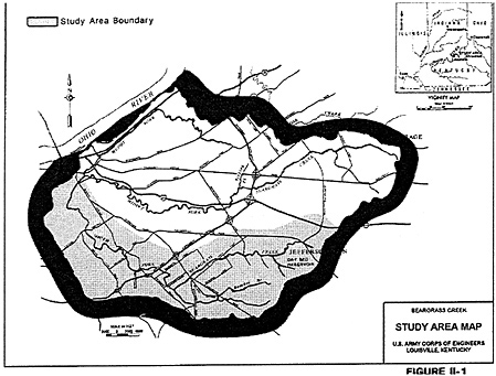
FIGURE 5.1 The Beargrass Creek basin in Louisville, Kentucky. SOURCE: USACE (1997a) (Figure II-1).

about 300 buildings and cause about $7 million in flood damages, while a 100-year flood will impact about 750 buildings and cause about $45 million in flood damages (USACE, 1997c). The expected annual flood damage under existing conditions is approximately $3 million per year.

Flood Damage Reduction Measures

Beargrass Creek has several flood damage reduction structures, the most notable of which is a very large levee at its outlet on the Ohio River ( Figure 5.2a ). This levee was built following a disastrous flood on the Ohio in January 1937, and the levee crest is an elevation of 3 feet above the 1937 flood level on the Ohio River. During the 1937 flood it was reported that “at the Public Library, the flood waters reached a height such that a Statue of Lincoln appeared to be walking on water!” (USACE, 1997b, p. III-2). Near the mouth of Beargrass Creek, a set of

gates can be closed to prevent water from the Ohio River from flowing back up into Louisville. In the event of such a flood, a massive pump station with a capacity of 7,800 cubic feet per second (cfs) is activated to discharge the flow of Beargrass Creek over the levee and into the Ohio River.

Between 1906 and 1943, a traditional channel improvement project was constructed on the lower reaches of the South Fork of Beargrass Creek. It consists of a concrete lined rectangular channel with vertical sides, with a small low-flow channel down the center ( Figure 5.2b ). The channel's flood conveyance capacity is perhaps twice that of the natural channel it replaced, but the concrete channel is a distinctive type of landscape feature that environmental concerns will no longer permit. Other structures have been added since then, including a dry bed reservoir completed in 1980, which functions as an in-stream detention basin during floods.

The proposed flood damage reduction measures for Beargrass Creek form an interesting contrast to traditional approaches. The emphasis of the proposed measures is on altering the natural channel as little as possible and detaining the floodwaters with detention basins. These basins are either located on the creek itself or more often in flood pool areas adjacent to the creek into which excessive waters can drain, be held for a few hours until the main flood has passed, and then gradually return to the creek. Figure 5.2c shows a grassed detention pond area with a concrete weir (in the center of the picture) adjacent to the creek. Figure 5.2d shows Beargrass Creek at this location (a discharge pipe from the pond is visible on the right side of the photograph). Water flows from the creek into the pond over the weir and discharges back into the creek through the pipe. The National Economic Development flood damage reduction alternative on Beargrass Creek called for a total of eight detention basins, one flood wall or levee, and one section of modified channel. Other alternatives such as flood-proofing, flood warning systems, and enlargement of bridge openings were considered but were not included in the final plan.

The evolution of flood damage reduction on Beargrass Creek represents an interesting mixture of the old and the new—massive levees and control structures on the Ohio River, traditional approaches (the concrete-lined channel) in the lower part of the basin, more modern instream and off-channel detention basins in the upstream areas, and local channel modifications and floodwalls. Maintenance and improvement of stormwater drainage facilities in Beargrass Creek are the responsibility of the Jefferson County Metropolitan Sewer District, which is the principal local partner working with the Corps to plan and develop flood damage reduction measures.

(a) Levee on the Ohio River

(b) Concrete-lined channel

(c) Detention pond

(d) Beargrass Creek at the detention pond

FIGURE 5.2 Images of Beargrass Creek at various locations: (a) the levee on the Ohio River, (b) a concrete-lined channel, (c) a detention pond, and (d) the Beargrass Creek at the detention pond.

In some locations, development has been prohibited in the floodway; but in other places, buildings are located adjacent to the creek. The Corps's feasibility report includes the following comments: “Urbanization continues to alter the character of the watershed as open land is converted to residential, commercial and industrial uses. The quest for open area residential settings in the late 1960s and early 1970s caused a tremendous increase in urbanization of the entire basin. Several developers have utilized the aesthetic beauty of the streambanks as sites for residential as well as commercial developments. This has resulted in increased runoff throughout the drainage area as development has occasionally encroached on the floodplain and, less frequently, the floodway” (USACE, 1997b, p. II-2).

Damage Reaches

To conduct the flood damage assessment, the two main creeks— South Fork of Beargrass Creek and Buechel Branch—are divided into damage reaches. Flood damage and risk assessment results are summarized for each damage reach, and the expected annual damage for the project as a whole is found by summing the expected annual damages for each reach. As shown in Figure 5.3 , the South Fork was divided into 15 damage reaches and the Buechel Branch into 5 reaches (a sixth damage reach on Buechel Branch is not shown in this figure). Approximately 12 miles of Beargrass Creek, and 2.2 miles of Buechel Branch are covered by the these damage reaches. The average length of a damage reach is thus 0.8 miles for the South Fork of the Beargrass Creek, and the average length for Buechel Branch is 0.4 miles. The shorter reaches on Buechel Branch are adjacent to similarly short, upstream reaches in Beargrass Creek where most flood damage occurs. Longer damage reaches are used downstream on Beargrass Creek where less damage occurs.

The highest expected annual flood damage is on Reach SF-9 on the upper portion of the South Fork of Beargrass Creek. Results from this damage reach are used for illustrative purposes at various points in this chapter.

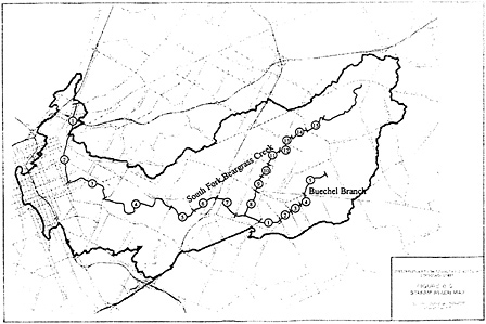
FIGURE 5.3 Damage reaches on the South Fork of Beargrass Creek and Buechel Branch. SOURCE: USACE (1997a) (Figure III-3).

Flood Hydrology

Most of the flood damage reduction measures being considered are detention basins, which diminish flood discharge by temporarily storing floodwater. It follows that the study's flood hydrology component has to be conducted using a time-varying rainfall–runoff model because this allows for the routing of storage water through detention basins. In this case, the HEC-1 rainfall–runoff model from the Corps's Hydrologic Engineering Center (HEC) was used to quantify the flood discharges. The Hydrologic Engineering Center has subsequently released a successor rainfall-runoff model to HEC-1, called HEC-HMS (Hydrologic Modeling System), which can also be used for this type of study (HEC, 1998b).

In each damage reach, and for each alternative plan considered, the risk analysis procedure for flood damage assessment requires a flood – frequency curve defining the annual maximum flood discharge at that location which is equaled or exceeded in any given year with a given probability. In this study all these flood–frequency curves were produced through rainfall–runoff modeling. In other words, a storm of a given

return period was used as input to the HEC-1 model, the water was routed through the basin, and the magnitude of the discharge at the top end of each damage reach was determined (Corps hydrologists have assumed, based on experience in the basin, that storms of given return periods produce floods of the equivalent return period). By repeating this exercise for each of the annual storm frequencies to be considered, a flood–frequency curve was produced for each damage reach. There are eight standard annual exceedance probabilities normally used to define this frequency curve: p = 0.5, 0.2, 0.1, 0.04, 0.02, 0.01, 0.004, and 0.002, corresponding to return periods of 2, 5, 10, 25, 50, 100, 250, and 500 years, respectively. In this study, because even small floods cause damage, a 1-year return period event was included in the analysis and assigned an exceedance probability of 0.999.

Considering that there are 21 damage reaches in the study area and 8 annual frequencies to be considered, each alternative plan considered requires the development of 21 flood–frequency curves involving 168 discharge estimates. During project planning, as dozens of alternative components and plans were considered, the sheer magnitude of the tasks of hydrologic simulation and data assembly becomes apparent.

The hydrologic analysis is further complicated by the fact that the design of detention basins is not simply a cut-and-dried matter. A basin designed to capture a 100-year flood requires a high–capacity outlet structure. Such a basin will have little impact on smaller floods because the outlet structure is so large that smaller events pass through almost unimpeded. If smaller floods are to be captured, a more confined outlet structure is needed, which in turn increases the required storage volume for larger floods. This situation was resolved in the Beargrass Creek study by settling on a 10-year flood as the nominal design event for sizing flood ponds and outlet works. The structures designed in this manner were then subjected to the whole range of floods required for the economic analysis.

Rainfall–Runoff Model

The HEC-1 model was validated by using historical rainfall and runoff data for four floods (March 1964, April 1970, July 1973, February 1990). Modeling results were within 5 percent to 10 percent of observed flows at two U.S. Geological Survey (USGS) streamflow gaging stations: South Fork of Beargrass Creek at Trevallian Way and Middle Fork

of Beargrass Creek at Old Cannons Lane, which have flow records beginning in 1940 and 1944, respectively, and continuing to the present. A total of 42 subbasins were used in the HEC-1 model, and runoff was computed using the U.S. Soil Conservation Service (renamed the Natural Resources Conservation Service in 1994) curve number loss rates and unit hydrographs. The Soil Conservation Service curve numbers were adjusted to allow the matching of observed and modeled flows for the historical events. A 6-hour design storm was used, which is about twice the time of concentration of the basin. The design storm duration chosen is longer than the time of concentration of the basin so that the flood hydrograph has time to rise and reach its peak outflow at the basin outlet while the storm is still continuing. If the design storm is shorter than the time of concentration, rainfall could have ceased in part of the basin before the outflow peaks at the basin outlet. The storm rainfall hydrograph was based on National Weather Service 1961 Technical Paper 40 (NWS, 1961) and on a Soil Conservation Service storm hydrograph, and a 5-minute time interval of computation was used for determining the design discharges.

There is a long flood record of 56 years of data (1940–1996) available in the study area (USGS gage on the South Fork of Beargrass Creek at Trevallian Way). A comparison was made of observed flood frequencies at this site with those simulated by HEC-1, with some adjustment of the older flood data to allow for later development. Traditional flood frequency analysis of observed flow data had little impact in the study. This may have been the case because there was only one gage available within the study area, or because the basin has changed so much over time that the flood record there does not represent homogeneous conditions. Furthermore, the alternatives mostly involve flood storage, which requires computation of the entire flood hydrograph, not just the peak discharge.

Uncertainty in Flood Discharge

Uncertainty in flood hydrology is represented by a range in the estimated flood–frequency curve at each damage reach. In the HEC-FDA program, there are two options for specifying this uncertainty: an analytical method based on the log-Pearson distribution and a more approximate graphical method. The log-Pearson distribution is a mathematical function used for flood–frequency analysis, the parameters of which are determined from the mean, standard deviation, and coefficient

of skewness of the logarithms of the annual maximum discharge data. The graphical method is a flood frequency analysis performed directly on the annual maximum discharge data without fitting them with a mathematical function. In this case the graphical method was used with an equivalent record length of 56 years of data, the length of the flood record of the USGS gage station at Trevallian Way at the time of the study. Figure 5.4 shows the flood–frequency curve for damage reach SF-9 on the South Fork of Beargrass Creek, with corresponding confidence limits based on ± 2 standard deviations about the mean curve.

The confidence limits in this graph are symmetric about the mean when the logarithm to base 10 of the discharge is taken, rather than the discharge itself. This can be expressed mathematically as:

where Q is the discharge value at the confidence limit, log Q is the expected flood discharge, σ log Q is the standard deviation (shown in the rightmost column of Table 5.1 ), and K is the number of standard deviations above or below the mean that the confidence limit lies. Because these confidence limits are defined in the log space, it follows that they are not symmetric in the real flood discharge space. As Table 5.1 shows, the expected discharge for the 100-year flood ( p = 0.01) is 4,310 cfs, the upper confidence limit is 6,176 cfs, and the lower limit is 3,008 cfs. The difference between the mean and the upper confidence limit is thus about 40 percent larger than the difference between the mean and the lower confidence limit. The confidence limits for graphical frequency analysis are computed using a method based on order statistics, as described in USACE (1997d). In this method, a given flood discharge estimate is considered a sample from a binomial distribution, whose parameters p and n are the nonexceedance probability of the flood and the equivalent record length of flood observations in the area, respectively. In this case, n = 56 years, since this is the record length of the Trevallian Way gage.

River Hydraulics

Water surface profiles for all events were determined using the HEC-2 river hydraulics program from the Corps's Hydrologic Engineering Center in Davis, California. Field-surveyed cross sections were obtained

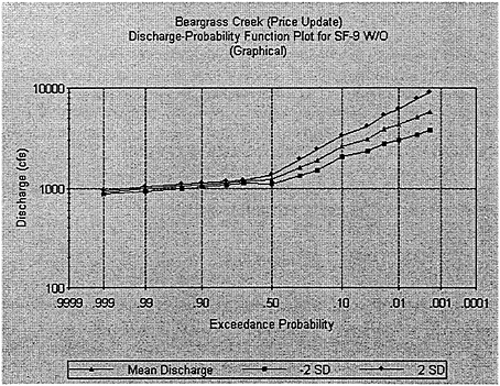
FIGURE 5.4 The flood–frequency curve and its uncertainty at damage reach SF-9 on the South Fork of Beargrass Creek.

at all bridges and at some stream sections near bridges. Maps with a scale of 1 inch = 100 feet with contour intervals of 2 feet were used to define cross sections elsewhere on the stream reaches and were used for measuring the distance between cross sections on the channel and in the left and right overbank areas. Manning's n values for roughness were based on field inspection, on reproduction of known high-water marks from the March 1964 flood on Beargrass Creek, and on reproduction of the rating curve of the USGS gage at Trevallian Way. Manning's equation relates the channel velocity to the channel's shape, slope, and roughness. Manning's n is a numerical value describing the channel roughness. Manning's n values in the concrete channel ranged from 0.015 at the channel invert to 0.027 near the top of the bank. In the natural channels, Manning 's n values ranged from 0.035 to 0.050. In the overbank areas, these values ranged from 0.045 to 0.065. Where buildings blocked the flow, the cross sections were cut off at the effective

TABLE 5.1 Uncertainties in Estimated Discharge Values at Reach SF-9

flow limits. A total of 201 cross sections were used for the South Fork of Beargrass Creek, and 61 cross sections were used for Buechel Branch. The average distance between cross sections was 330 feet on the South Fork of Beargrass Creek and 245 feet on Buechel Branch. Cross sections are spaced more closely than this near bridges and more sparsely in reaches where the cross section is relatively constant.

Figure 5.5 shows the water surface profiles along Beargrass Creek for the eight flood frequencies considered, under existing conditions without any planned control measures. The horizontal axis of this graph is the distance in miles upstream from Beargrass Creek's outlet on the Ohio River. The vertical axis is the elevation of the water surface in feet above mean sea level. The bottom profile in this graph is the channel invert or channel bottom elevation. The top profile is for p = 0.002—the 500-year flood. This particular profile shows a sharp drop near the bottom end of the channel, caused by a bridge at that location that constricts the flow. The flat water surface elevation upstream of the bridge is a backwater effect produced by the inadequate capacity of the bridge opening to convey the flow that comes to it.

For each flood profile computed, the number of structures flooded and the degree to which they are flooded must be assessed. Figure 5.6 shows the locations of the first-floor elevations of structures affected by flooding on the South Fork of Beargrass Creek in relation to several flood water surface profiles under existing conditions. Damage reach SF-9 is located between river miles (RM) 9.960 and 10.363, near the point where there is a sharp drop in the channel bed and water surface elevation on Beargrass Creek. It can be seen that the density of development varies along the channel. Flood damage reduction measures are most effective when they are located close to damage reaches with significant numbers of structures, and they are least effective when they are distant from such reaches.

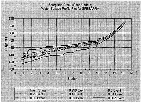
FIGURE 5.5 Water surface profiles for design floods in Beargrass Creek under existing conditions.

Each damage reach has an index location, which is an equivalent point at which all of the damages along the reach are assumed to occur. On reach SF-9, this index location is at river mile 10.124. To assess damages to structures within each reach, an equivalent elevation is found for each structure at the index location such that its depth of flooding at that location is the same as it would have been at the correct location on the flood profile, as shown in Figure 5.7 .

The technique of assigning an elevation at the index location can be far more complex than Figure 5.7 implies, because allowance is made in the HEC-FDA program for the various flood profiles to be nonparallel and also to change in gradient upstream of the index location compared to downstream. In the Beargrass Creek study, a single flood profile for the p = 0.01 event was chosen, and all other profiles were assumed parallel to this one. One damage reach on Beargrass Creek was subdivided into three subreaches to make this assumption more nearly correct. A spatial distribution of buildings over the damage reach is thus converted

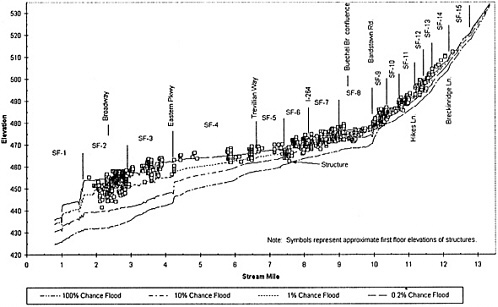
FIGURE 5.6 Locations of structures on floodwater surface profiles along the damage reaches of the South Fork of Beargrass Creek. SOURCE: USACE, 1997c.

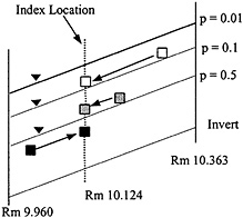
FIGURE 5.7 Assignment of structures to an index location.

into a probability distribution of buildings at the index location, where the uncertainty in flood stage is quantified.

Uncertainty in Flood Stage

The uncertainty in the water surface elevation was quantified by assuming that the standard deviation of the elevation at the index location for the 100-year discharge is 0.5 feet. The 100-year discharge at reach SF-9 is 4,310 cfs, which is the next to last set of points in Fugure 5.8 . To the right of these points, between the 100-year and 500-year flood discharges, the uncertainties are assumed to be constant. For discharges lower than the 100-year return period, the uncertainties in stage height are reduced linearly in proportion to the depth of water in the channel. The various lines shown in Figure 5.8 are drawn as the expected water surface elevation ± 1 or 2 standard deviations determined in this manner.

Economic Analysis

The Corps's analysis of a flood damage reduction project's economic costs and benefits is guided by the Principles and Guidelines ( Box 1.1 provides details on the P&G's application to flood damage reduction

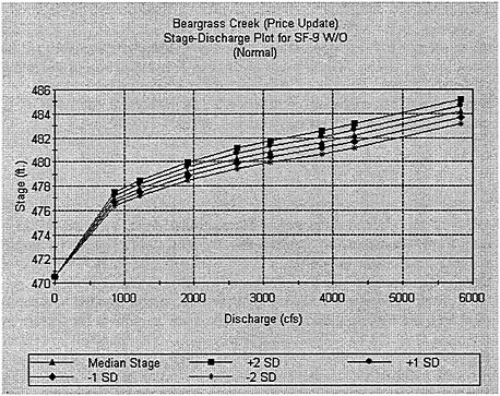
FIGURE 5.8 Uncertainty in the flood stage for existing conditions at reach SF-9 of the South Fork of Beargrass Creek.

studies). According to the P&G , the economic analysis of damages avoided to floodplain structures because of a flood damage reduction project is restricted to existing structures (i.e., federal policy does not allow damages avoided to prospective future structures to be counted as benefits). The P&G do, however, call for the benefits of increased net income generated by floodplain activities after a project has been constructed (so-called “intensification benefits”) to be included in the economic analysis.

Economic analysis of flood damages considers various sorts of flood damage, principal among them being the damage to flooded structures. Information about the structures is quantified using a “structure inventory,” an exhaustive tabulation of every building and other kind of structure subjected to flooding in the study region. A separate computer program called Structure Inventory for Damage Analysis (SID) was used

to evaluate the number of structures flooded as a function of water surface elevation. Structures are divided into four categories: single-family residential, multifamily residential, commercial, and public. A structure is considered to be flooded if the computed flood elevation is above its first-floor elevation. The amount of damage D is a function of the depth of flooding h and the type of structure, and is expressed by a factor, r ( h ), which is equal to a percentage of the value of the structure ( V ) and of its contents (C). This analysis can be expressed as

D = r 1 ( h ) V + r 2 ( h ) C . (5.2)

For residential structures, these damage factors were quantified in 1995 by the Federal Emergency Management Agency (FEMA) using data from flood damage claims. For example, for a one-story house without a basement flooded to a depth of 3 feet, the FEMA estimate is that the damage factors are r 1 = 27% of the value of the structure and r 2 = 35% of the value of the contents. For the same house flooded to a depth of 6 feet, the corresponding damage factors are r 1 = 40% for the structure, and r 2 = 45% for the contents, respectively. The Marshall and Swift Residential Cost Handbook (Marshall and Swift, 1999) was used to estimate the value of single- and multi-family structures (it bears mentioning that the use of standard references such as the Marshall and Swift handbook may potentially represent another source of “knowledge uncertainty ”). The values of their contents were assumed to be 40 percent to 44 percent of the value of the structure. For commercial and public buildings, the values of the structures and their contents were established through personal interviews by Corps personnel. About 85 percent of the structures subject to flood damage are residential buildings.

Types of flood damages beyond those to structures were also considered. For instance, there are several automobile sales lots in the floodplain, and prospective damages to cars parked there during a flood were estimated. Nonphysical damage costs include the costs of emergency services and traffic diversion during flooding. Damage to roads and utilities were also considered.

Uncertainty in Flood Damage

The economic analysis has three sources of uncertainty:

the elevation of the first floor of the building,

the degree of damage given the depth of flooding within the building, and

the economic value of the structure and its contents.

For most structures in Beargrass Creek, the first-floor elevation was estimated from the ground elevation on maps with a scale of 1 inch = 100 feet and with contour intervals of 2 feet. For a sample of 195 structures (16% of the total number), the first-floor elevations were surveyed. It was found that the average difference between estimated and surveyed first-floor elevations of these structures was 0.62 feet.

Corps Engineering Manual (EM) 1110-2-1619 (USACE, 1996b) was used to estimate values for the uncertainties in economic analysis. A standard deviation of 0.2 feet was used to define the uncertainty in first-floor elevations. The uncertainty in the degree of damage given a depth of inundation was estimated by varying the percent damage factor described previously. For residential structures the value of the structure was assigned a standard deviation of 10 percent of the building value, and the ratio of the value of the contents to the structure was allowed to vary with a standard deviation of 20 percent to 25 percent.

For commercial property a separate damage estimate, based on interviews with the owners, was made for each significant property and was expressed as a triangular distribution with a minimum, expected, and maximum damage value for the property. Because every individual structure potentially affected by flooding is inventoried in the damage estimate data, the amount of work required to collect all these damage data was extensive.

The end result of these estimates at each damage reach and damage category is a damage–stage curve (such as Figure 5.9 ) that accumulates the damage to all multifamily structures in this damage reach for various water surface elevations at the index location, denoted by stage on the horizontal axis. This curve is prepared by first dividing the range of the stage (476–486 feet) into increments —increments of 0.5 feet in this case. For each structure, a cycle of 100 Monte Carlo simulations is carried out in which the first-floor elevation and the values of the structure and contents are randomly varied. From these simulations estimates are formed for each 0.5-foot stage height increment of what the expected damage and standard deviation of the damage to that structure would be if the flood stage were to rise to that elevation. For each stage increment, these means and standard deviations are accumulated over all structures in the

reach to form the estimate of the mean and standard deviation of the reach damage ( Figure 5.9 ).

A similar function is prepared for each of the damage categories. At any flood stage, the sum of the damages across all categories is the total flood damage for that reach.

Project Planning

The discussion of the Beargrass Creek study reviewed the technical means by which a particular flood damage reduction plan is evaluated. A plan consists of a set of flood damage reduction measures, such as detention ponds, levees or floodwalls, and channel modifications, implemented at particular locations on the creek. The base plan against which all others are considered is the “without plan,” which means a plan that considers existing conditions in the floodplain and the development expected to occur even in the absence of a flood damage reduction plan. Such development must meet floodplain management policies and have structures elevated out of the 100-year floodplain. A base year of 1996 was chosen for the Beargrass Creek study.

In carrying out project planning, the spatial location of the principal damage reaches is important because flood damage reduction measures located just upstream of or within such reaches have greater economic impact than do flood damage reduction measures located in areas of low flood damage. Project planning also involves a great deal of interaction with local and state agencies, in this case principally the Jefferson County Metropolitan Sewer District.

The Beargrass Creek project planning team consisted primarily of three individuals in the Corps's Louisville district office: a project planner from the planning division, a hydraulic engineer from the hydrology and hydraulics design section, and an economic analyst from the economics branch. The HEC-FDA computer program with risk analysis was carried out by the economic analyst using flood–frequency curves and water surface profiles supplied by the hydrology and hydraulics section and using project alternatives defined by the project planner. The hydrology and hydraulics section was also responsible for the preliminary sizing of potential project structures being considered as plan components. The bulk of the work of implementing the risk analysis aspects of flood damage assessment thus fell within the domain of the Corps economic analyst.

The HEC-FDA program is applied during the feasibility phase of

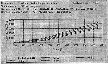
FIGURE 5.9 The damage–stage curve with uncertainty for multifamily residential property in Reach SF-9 of the South Fork of Beargrass Creek.

flood damage reduction planning. This had been preceded by a reconnaissance phase, a preliminary assessment of whether reasonable flood damage reduction planning can be done in the area. As explained in Chapter 2 , the reconnaissance phase is fully funded by the federal government, but the feasibility phase must have half the costs met by a local sponsor. Assuming the feasibility phase yields an acceptable plan and additional funds are authorized, the project proceeds to a detailed design and construction phase, which also requires local cost sharing. The Beargrass Creek project is now (as of May 2000) in the detailed design phase.

Evaluation of Project Alternatives

Expected annual flood damages in Beargrass Creek under existing conditions are estimated to be $3 million. Project benefits are calculated as the difference between this figure and the lower expected annual damages that result with project components in place. Project costs are annualized values of construction costs discounted over a 50-year period using an interest rate of 7.625 percent. Project net benefits are the differ-

ence between project benefits and costs. For components to be included in the project, they must have positive net benefits.

The first step in evaluating project alternatives is to consider each component flood damage reduction measure by itself to see if it yields positive net benefits. A total of 22 components were examined individually, 11 on the South Fork of Beargrass Creek and 11 on Buechel Branch. All 11 of the South Fork components were economically justified on a stand-alone basis. Only 3 of the 11 components on Buechel Branch were justified individually: the other 8 components were thus deleted from further consideration.

The next step is to formulate the National Economic Development (NED) plan. In theory, this is supposed to proceed by selecting first the component with the largest net benefits, adding the component with the next largest net benefits, evaluating them together, and continuing to add more components until the combined set of components has the largest overall net benefits. It turned out that this idealized approach could not be used at the South Fork of Beargrass Creek because of economic and hydraulic interactions among the components. The study team commented: “Therefore, the formulation process was different and more complicated than originally anticipated. The study team could not follow the incremental analysis procedure to build up the NED plan because the process became a loop of H&H computer runs. Our component with the greatest net benefits is located near the midpoint of the stream; thus, each time we would add a component upstream it would affect all components downstream and vice versa. We could never truly optimize or identify the plan which produces the greatest net benefits” (USACE, 1997c, p. IV-62).

The problems were further complicated by the fact that there are three separate sections of the study region: the South Fork of Beargrass Creek and Buechel Branch upstream of their junction and the South Fork downstream of this junction ( Figure 5.3 ). In the downstream region, flood damage reduction measures on the upper South Fork and Buechel Branch compete for project benefits by reducing flood damages. The result of these complications is that the plan was built up incrementally by separately considering the three sections of the region. First, the most upstream control structure in each section was selected, then structures downstream were added. At the end—when the components from the three sections had been aggregated into a single overall plan—it was determined whether the plan could be improved by omitting individual marginal components. The end result of this iterative process was a recommended plan with 10 components: 8 detention basins, 1 floodwall,

and 1 channel improvement.

Each plan has to be evaluated using the Monte Carlo simulation process. The number of simulations varies by reach, with 10,000 required for Reach SF-9 and with a range of 10,000–100,000 required for the other reaches. On a 300 MHz Pentium computer, evaluation of a single plan takes about 25 minutes of computation time.

Risk of Flooding

The HEC-FDA program also produces a set of statistics that quantify the risk of being flooded in any reach for a given plan, as shown in Table 5.2 . For reach SF-9, the target elevation is 477.2 feet, which is the elevation of the overbank area in this reach. The probability estimates shown are annual exceedance probability and conditional nonexceedance probability. The annual exceedance probability refers to the risk that flooding will occur considering all possible floods in any year. The conditional nonexceedance probability describes the likelihood that flooding will not occur during a flood of defined severity, such as the 100-year (1 percent chance) flood.

There is a subtle but important distinction between these two types of risk measures. The annual exceedance probability accumulates all the uncertainties into a single estimate both from the natural variability of the unknown severity of floods and from the knowledge uncertainty in estimating methods and computational parameters. The conditional non-exceedance probability estimate divides these two uncertainties, because it is conditional on the severity of the natural event and thus represents only the knowledge uncertainty component. In this sense, the conditional nonexceedance probability corresponds most closely to the traditional idea of adding 1 foot or 3 feet on the 100-year base flood elevation, while the annual exceedance probability corresponds more closely to the goal of ensuring that the chance of being flooded is less than a given value, such as 1 percent, considering all sources of uncertainty.

The “target stage annual exceedance probability” values in Table 5.2 are the median and the expected value or mean of the chance that flooding will occur in any given year for the various reaches. Thus, for reach SF-9, there is approximately a 36 percent chance that flooding will occur beyond the target stage in any given year, while in reach SF-14 upstream, that chance is only about 9 percent. The “long term risk” values in the

TABLE 5.2 Risk of Flooding in Damage Reaches Calculated Uncertainty for 1996 at Beargrass Creek

figure refer to the chance (Rn) that there will be flooding above the target stage at least once in n years, determined by the formula

R n = 1− (1− p e ) n , (5.3)

where p e is the expected annual exceedance probability. For example, for reach SF-9, where p e = 0.3640, for n = 10 years, R 10 = 1− (1 − 0.3640) 10 = 0.9892, as shown in Table 5.2 .

The conditional nonexceedance probability values shown on the right-hand side of Table 5.2 are conditional risk values that correspond to the reliability that particular floods can be conveyed without causing damage in this reach. Thus, in reach SF-9, a 10 percent chance event (10-year flood) has about a 0.27 percent chance of being conveyed without exceeding the target stage, while for a 1 percent chance event (100-year flood), there is essentially no chance that it will pass without exceeding the target stage. By contrast, in Reach SF-14 at the upstream end of the study area, the conditional nonexceedance probability of the reach passing the 10-year flood is about 52 percent; that of the reach passing the 100-year flood is about 100 percent. As the flood severity increases, the chance of a reach being passed without flooding diminishes.

Effect on Project Economics of Including Risk and Uncertainty

The HEC-FDA program that includes risk and uncertainty factors in project analysis became available to the Beargrass creek project team late in the study period. Before then, the team used an earlier economic analysis program (Expected Annual Damage, or EAD) which computed expected annual damages without these uncertainties. O' Leary (1997) presented the data shown in Table 5.3 to compare the two approaches. It is evident that including risk and uncertainty increases the expected annual damage both with and without flood damage reduction plans. The net effect of their inclusion on the Beargrass Creek project is to increase the annual flood damage reduction benefits from $2.078 million to $2.314 million. The study team made a comparison between the components included in the National Economic Development plan in the two computer programs and found that there was no change. Hence, although the inclusion of risk and uncertainty increased project benefits, it did not result in changing the flood damage reduction components included in the National Economic Development plan.

O'Leary (1997) also presented statistics of the project benefits derived from the HEC-FDA program for the National Economic Development plan. The expected annual benefits of the National Economic Development plan—$2.314 million—are the same in Table 5.3 and Table 5.4 . The net benefits in the fourth column of Table 5.4 are found by subtracting the annual project costs from the expected annual benefits; the benefit-to-cost ratio is the ratio of the expected benefits to costs.

The 25 th percentile, median (50 th percentile), and 75 th percentile of the expected annual benefits are also shown. The project net benefits are positive at all levels of assessment, and all benefit-to-cost ratios are greater than 1.00. It is interesting to see that the median expected annual benefits ($2.071 million) are nearly the same as the expected value of these benefits without considering uncertainty ($2.078 million). Moreover, the expected value ($2.314 million) is greater than the median, and the difference between the 75 th percentile and the median is greater than the difference between the median and the 25 th percentile. All these characteristics point to the fact that the distributions of flood damages and of expected annual benefits are positively skewed when uncertainties in project hydrology, hydraulics, and economics are considered. This is why the project benefits increase when these uncertainties are considered. The project benefits for the 25 th percentile, 50 th percentile, and 75 th percentile in Table 5.4 should be read with caution because they are compiled for the project by adding together the corresponding values for all the damage reaches. The percentile value of a sum of random variables is not necessarily equal to the sum of the percentile values of each variable.

TABLE 5.3 Expected Annual Damages (EAD) With and Without Uncertainty in Damage Computations (millions of dollars per year)

TABLE 5.4 Statistics of project benefits under the NED plan using the HEC-FDA Program

RED RIVER OF THE NORTH AT EAST GRAND FORKS, MINNESOTA, AND GRAND FORKS, NORTH DAKOTA

A devastating flood occurred at East Grand Forks, Minnesota, and Grand Forks, North Dakota, in April 1997. After the flood, flood damage reduction studies previously done for the two cities were combined into a joint study, and risk analysis was performed to evaluate the reliability of the proposed alternatives and to evaluate their economic impacts. A risk analysis study performed before the flood was presented in a paper at the Corps's 1997 Pacific Grove, California, workshop (Lesher and Foley, 1997). This paper and subsequent analysis (USACE, 1998a, b, c), as well as a visit to the Corps's St. Paul district office by a member of this committee, form the basis of this discussion of the East Grand Forks–Grand Forks study.

East Grand Forks, Minnesota, and Grand Forks, North Dakota, are located on opposite banks of the Red River of the North and are approximately 300 miles above the river's mouth at Lake Winnipeg, Manitoba, Canada ( Figure 5.10 ). The East Grand Forks–Grand Forks metropolitan area has a population of approximately 60,000 and is located about 100 miles south of the U.S.–Canadian border. The total drainage area of the East Grand Forks–Grand Forks basin is 30,100 square miles. Included in this drainage area is the Red Lake River subbasin that effectively drains about 3,700 square miles in Minnesota and joins the mainstream of the Red River at East Grand Forks. The study area of East Grand Forks–Grand Forks lies in the middle of the Red

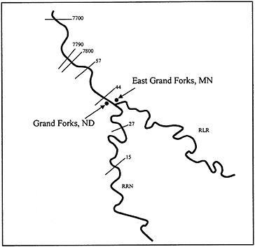
FIGURE 5.10 Schematic of the Red River of the North (RRN) and Red Lake River (RLR) at the East Grand Forks, Minnesota and Grand Forks, North Dakota study area. Numbers indicate USGS stream gages.

River Valley. The valley is exceptionally flat with a gradient that slopes 3–10 feet per mile toward the river with the north–south axis having a gradient of about three-quarters of a foot per mile. The valley extends approximately 23 miles west and 35 miles east of East Grand Forks– Grand Forks and is a former glacial lake bed.

Both cities have a long history of significant flooding from the Red River of the North and the Red Lake River. The most damaging flood of record occurred in April 1997 (see Table 5.5 ), when the temporary levee systems and flood-fighting efforts of both communities could not hold back the floodwaters of the Red River. The resulting damages were disastrous and affected both cities dramatically. Total damages to existing structures and contents during the 1997 flood were estimated to exceed $800 million. An additional $240 million was spent for emergency-related costs.

TABLE 5.5 Maximum Recorded Instantaneous Peak Flows; Red River of the North at Grant Forks, North Dakota

Risk Analysis

A risk analysis for the proposed flood damage reduction project for the Red River of the North at East Grand Forks, Minnesota, and Grand Forks, North Dakota, used a Latin Hypercube analysis to sample interactions among uncertain relationships associated with flood discharge and elevation estimation. Latin Hypercube is a stratified sampling technique used in simulation modeling. Stratified sampling techniques, as opposed to Monte Carlo-type techniques, tend to force convergence of a sampled distribution in fewer samples. Because the Hydrologic Engineering Center Flood Damage Analysis program (HEC-FDA) was new at the time, and in the interest of saving time, the analysis was performed using a spreadsheet template. The flood damage reduction alternatives analyzed included levees of various heights and a diversion channel in conjunction with levees. The project reliability option in the HEC risk spreadsheet was used to determine the reliability of the alternative levee heights and of the diversion channel in conjunction with levees. The following sections discuss the sensitivity in quantifying the uncertainties and the representation of risk for the alternatives.

Discharge–Frequency Relationships

The log-Pearson Type III distribution, recommended in the Water Resource Council's Bulletin 17B (IACWD, 1981) and incorporated

within the Corps's HEC Flood Frequency Analysis (HEC-FFA) computer program, was used for frequency analysis of maximum annual streamflows, and the noncentral t distribution was used for the development of confidence limits. Discharge–frequency relationships were needed for both the levees and the diversion channel in combination with levees. An analysis (coincidental frequency) was performed to develop the discharge– frequency curves for the Red River of the North downstream and upstream of the Red Lake River for the levees only condition. A graphical method was used to develop the discharge–frequency curves for the diversion channel in combination with levees. Details of these procedures can be found in a Corps instruction manual from the St. Paul district (USACE, 1998a). A brief discussion of these procedures is provided below.

The Grand Forks USGS stream gage (XS 44) is currently located 0.4 miles downstream from the Red Lake River in Grand Forks, North Dakota ( Figure 5.10 ). The discharge–frequency curve for this station along with the 95 percent and 5 percent confidence limits (90% confidence band) are plotted in Figure 5.11 . An illustration of the noncentral t probability density function for the 1 percent event is also shown in that figure. Selected quantities of that discharge–frequency relationship are shown in column 2 of Table 5.6 . The coincidental discharge–frequency relationship for the Red River just upstream of the mouth of the Red Lake River (column 3 of Table 5.6 ) was computed with the HEC-FFA computer program. The basic flow values were obtained by routing the 96 years of available data on Red Lake River flows from Crookston (55 miles upstream of the mouth) downstream to Grand Forks. The resulting flows were subtracted from the Red River at Grand Forks flows to obtain coincident discharges on the Red River upstream of Red Lake River. The two-station comparison method of Bulletin 17B was used to adjust the logarithmic mean and standard deviation of this short record (96 years) based on regression analysis with the long-term record at the Grand Forks station (172 years). Correlation of coincident flows for the short record with concurrent peak flows for the long record produced a correlation coefficient of 0.975.

Adjustment of the statistics yielded an equivalent record length of 165 years. The adopted coincidental discharge–frequency curve for the Red River upstream of the Red Lake River is shown in column 3 of Table 5.6 for selected annual exceedance probabilities. The coincidental discharge –frequency curve for the Red Lake River at the mouth was determined by computing the difference in Red River flows both upstream and downstream of Red Lake River (see column 4 in Table 5.6 ). Statistics for the adopted relationship were approximated by synthetic methods presented in Bulletin 17B (for more details, see USACE (1998a)).

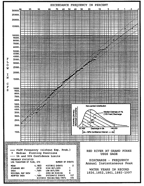
FIGURE 5.11 Flood (discharge) frequency curve for the Red River at Grand Forks.

TABLE 5.6 Instantaneous Annual Peak Discharges (cfs) and their Annual Exceedance Probabilities (%) — Existing Conditions

and downstream of Red Lake River (see column 4 in Table 5.6). Statistics for the adopted relationship were approximated by synthetic methods presented in Bulletin 17B (for more details, see USACE (1998a)).

The Plan Comparison Letter Report developed in February 1998 for flood damage reduction studies for East Grand Forks, Minnesota, and Grand Forks, North Dakota, evaluated an alternative flood damage reduction plan that included a split-flow diversion channel along with permanent levees. The discharge–frequency relationships for the modified conditions, shown in Table 5.7 , were developed as follows. The modified-condition discharge–frequency curve for the Red River upstream of Red Lake River was graphically developed based upon the operation of the diversion channel inlet. Red River flows are not diverted until floods start to exceed those having return periods of 5 years (20% annual exceedance probability). The channel is designed to continue to divert Red River flows at a rate that allows the design flood (0.47%) discharge of 102,000 cfs (upstream of the diversion) to be split such that 50,500 cfs is diverted and 51,500 cfs is passed through the cities. This operation is reflected in the modified discharge–frequency relationship shown in Table 5.7 for the Red River upstream of Red Lake River (columns 2 and

TABLE 5.7 Instantaneous Annual Peak Discharges (cfs) and their Annual Exceedance Probabilities (%)—Condition with Diversion Channels

3).Synthetic statistics (mean, standard deviation, and skewness) in accordance with methodology presented in Bulletin 17B were computed for the discharge-frequency relationships of the below-diversion flows.

The modified-condition discharge–frequency curve for the Red River downstream of Red Lake River was graphically computed based upon the operation of the diversion channel. The modified-condition Red River discharges upstream of Red River were added to the coincident flows on Red Lake River (column 4). The resulting discharges were plotted for graphical development of the modified-condition discharge– frequency relationship for the Red River downstream of Red Lake River and are summarized in Table 5.7 (column 5). Synthetic statistics for this discharge–frequency relationship were computed for use in the risk analysis.

Elevation–Discharge Relationships

The water surface elevations computed using the HEC-2 computer program are shown in Table 5.8 for three cross sections (7790, 7800, and 7922) corresponding to the previous USGS gage locations and for cross

section 44, which corresponds to the current USGS gage location (see Figure 5.10 for the cross section locations). These computed water surface elevations (CWSE) were based on the expected discharge quantities from the coincidental frequency analysis performed in June 1994 for the Grand Forks Feasibility Study. These data were used to transfer observed elevations from previous USGS gage sites to the current site (cross section 44) at river mile 297.65, and they were used in determining the elevation –discharge uncertainty. The water surface profile analysis was performed using cross-sectional data obtained from field surveys. Data were also obtained from field surveys and from USGS topographic maps. The HEC-2 model was calibrated to the USGS stream gage data and to high-water marks for the 1969, 1975, 1978, 1979 and 1989 flood events throughout the study area. Note that these water surface elevations assume the existing East Grand Forks and Grand Forks emergency levees are effective. The levees were assumed effective because through extraordinary efforts, they have generally been effective for past floods with the exception of the 1997 flood.

Ratings at stream gage locations provide an opportunity to directly analyze elevation–discharge uncertainty. The measured data are used to derive the “best fit” elevation-discharge rating at the stream gage location, which generally represents the most reliable information available. In this study, the adopted rating curve for computing elevation uncertainty is based on the computed water surface elevations from the calibrated HEC-2 model shown in Table 5.8 .

This adopted rating curve for cross section 44 at the current USGS gage is shown in Figure 5.12 . Measurements at the gage location were used directly to assess the uncertainty of the elevation–discharge relationship. The normal distribution was used to describe the distribution of error from the “best-fit” elevation–discharge rating curve. The observed gage data (for the four cross sections presented in Table 5.8 ) were transferred to the current gage site at river mile 297.65 based on the gage location adjustments presented in Table 5.9 , which were computed from the water surface elevations in Table 5.8 . These adjustments were plotted against the corresponding discharge below the Red Lake River, and curves were developed to obtain adjustments for other discharges.

The deviations of the observed elevations from the fitted curve were used to estimate the uncertainty of the elevation–discharge rating curve shown in Figure 5.11 . The deviations reflect the uncertainty in data values as a result of changes in flow regime, bed form, roughness/resistance to flow, and other factors inherent to flow in natural streams. Errors also

TABLE 5.8 Computed Water Surface Elevations of the Red River of the North at Grand Forks, North Dakota (units in feet above sea level)

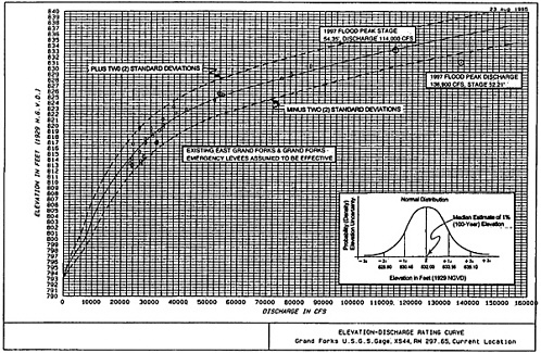
FIGURE 5.12 Rating curve (water elevation vs. discharge)for the Red River at Grand Forks.

TABLE 5.9 Adjustments Used in Transferring Observed Elevations from Previous USGS Gage Sites to Current Gage Site at RM 297.65 (XS 44)

result from field measurements or malfunctioning equipment. A minimum of 8–10 measurements is normally required for meaningful results. The measure used to define the elevation–discharge relationship uncertainty is the standard deviation:

Where X = observed elevation adjusted to current gage location (if 5.12 necessary), M = computed elevation from adopted rating curve, and N = number of measured discharge values (events).

The elevation uncertainty was computed for two different discharge ranges for this analysis. Based on the observed elevations plotted on the adopted rating curve, it appeared that there was greater uncertainty for discharges less than about 10% of annual exceedance probability event due to ice effects on flow. Therefore, the standard deviation was computed for discharges greater than between 22,000 cfs, which corresponds approximately to the zero damage elevation based on the adopted rating curve, and 44,000 cfs, which is slightly greater than the 10 percent annual exceedance probability. The standard deviation was also computed for discharges greater than 50,000 cfs. During the period of record, there were 25 events with a discharge between 22,000 and 44,000 cfs and 10 events with a discharge greater than 50,000 cfs. The standard deviation was 1.66 feet for discharges between 22,000 and 44,000 cfs and was 1.55

feet for discharges greater than 50,000 cfs. In the risk and uncertainty simulations, the standard deviation was linearly interpolated between 1.66 and 1.55 feet for discharges between 44,000 and 50,000 cfs. (See USACE (1998b) for more details.)

In an earlier risk analysis that was performed for the Grand Forks Feasibility Study, a much lower standard deviation of 0.50 feet was used for discharges greater than 50,000 cfs. However, adding the 1997 flood to the analysis resulted in a standard deviation of 1.55 feet, which is similar to that computed for discharges less than 44,000 cfs. It should be noted that the discharge and elevation used in this analysis for the 1997 flood was the peak discharge of 136,900 cfs occurring on April 18, 1997 (see Table 5.4 ), and an elevation of 831.21 feet (Stage 52.21). The peak elevation of 833.35 feet (Stage 54.35) occurred on April 22, 1997 at a discharge of 114,000 cfs. The elevation of 831.21 feet was almost 5 feet below the rating curve at a discharge of 136,900 cfs; however, the peak elevation of 833.35 feet at a discharge of 114,000 cfs was essentially on the adopted rating curve. Both of these points are plotted on the rating curve in Figure 5.12 . Lines representing ± 2 standard deviations for the normal distribution, which encompasses approximately 95 percent of all possible outcomes, are also shown on the rating curve. An illustration of the normal distribution at the 1 percent (100-year) event for the project levee condition is also shown in Figure 5.12 .

Risk and Uncertainty Analysis Results

Four index locations were selected to evaluate project performance and project sizing. These locations are cross sections 57, 44 (current USGS gage), 27, and 15 ( Figure 5.10 ). The four locations were selected based on economic requirements for project sizing (see USACE, 1998c). The elevation–discharge rating curves (based on HEC-2 analysis) for existing and project conditions at these locations can be found in the USACE (1998b). Each of these rating curves shows three conditions, where applicable: (1) existing conditions, (2) removal of the pedestrian bridge at cross sections 7920-7922 and with project levees (“levee only”); and (3) with removal of the pedestrian bridge, with project levees, and with the diversion channel (“diversion channel”). Existing conditions means that the existing emergency levees are assumed to be effective up to and including the 5 percent (20-year) event and are ineffective for larger floods. The 5 percent (20-year) event was selected based

on comparison of water surface profiles with effective and probable failure point (PFP) levee elevations provided by the Geotechnical Design Section analysis (see USACE, 1998b, paragraph A.2.11 and Appendix B of this report). The pedestrian bridge was removed based on input from the cities of East Grand Forks and Grand Forks. The rating curves for the diversion channel alternative were based on limited information. The Red River to the North would start to divert into the diversion channel at the 20 percent (5-year) flood; therefore, up to this point the rating curve for existing conditions with levees was used.

An additional location was also selected to evaluate the performance of the levee only and diversion channel with 1 percent (100-year) levee alternatives. This location is at cross section 7700 at the downstream end of the project levees (see Figure 5.10 ). Cross section 7700 was selected based on hydraulic analysis as the least critical location—the location where the levees in combination with the diversion channel would first overtop from downstream backwater (see USACE, 1998b).

Project Reliability

The project reliability results are summarized in Table 5.10 , Table 5.11 through Table 5.12 . Table 5.9 contains the results for the levees-only alternatives. Table 5.11 contains the results for the diversion channel in combination with 1 percent (100-year) levees. Note that in Table 5.10 , three different alternative top-of-levee heights are evaluated, whereas in Table 5.11 , it is always the same alternative—diversion channel with 1 percent levees— but for the three different events. The top-of-levee elevations were computed based on a water surface elevation profile to ensure initial overtopping would occur at the least-critical location (here, cross section 7700). The downstream top-of-levee elevations were selected with the intent of having 90 percent probability of containing the specified flood and were based on previous risk analysis for the Grand Forks Feasibility Study preliminarily updated to include the 1997 flood. The 2 percent (50-year), 1 percent (100-year), and 0.47 percent (210-year/1997 flood) top-of-levee profiles are 3.2, 3.4, and 2.7 feet above their respective water surface profiles at the downstream end ( Table 5.10 ).

As seen in Table 5.10 , the intent of having 90 percent probability of containing the specified flood is generally realized. The 2 percent levees have a 92 percent probability of containing the 2 percent flood. The 1 percent levees have a 90 percent probability of containing the 1 percent

flood. The 0.47 percent levees have an 87 percent probability of containing the 0.47 percent flood.

TABLE 5.10 Reliability at Top of Levee for Three Top-of-Levee Heights

TABLE 5.11 Project Reliability at Top of Levee for Diversion Channel with 1 Percent (100-Year) Levees for Three Different Events

Reliability results for the diversion channel with 1 percent levees are summarized in Table 5.11 . Note again that the levees constructed in combination with the diversion are the same as for the 1 percent flood without the diversion channel and are the same for all three floods analyzed. As seen in the table, there is a 99 percent or greater probability of containing the flood for all three floods considered when the project includes the diversion channel.

As previously noted, the most critical location for project performance is at cross section 7700 at the downstream end of the project. Table 5.12

summarizes the results for all the alternatives considered and for numerous floods. The probability of the diversion channel in combination with 1 percent levees for the 0.2 percent event is listed in the table as greater than 95%. A more specific reliability was not cited for the 0.2 percent event for two reasons: (1) the discharge–frequency curve based on the approximate statistics starts to diverge from the graphical curve for extreme events and, (2) there was limited information available to develop the Red River to the North rating curves for the diversion alternative. These reasons are also why more extreme events were not analyzed.

TABLE 5.12 Conditional Exceedance Probability of Alternative for Various Events (based on analysis at downstream end of project—XS 7700)

Table 5.13 presents the simulated conditional exceedance probabilities from the economic project sizing analysis. The without-project condition is also included in this table for comparison purposes. The without-project condition is based on a zero damage elevation of 824.5 feet, assumes credit is given to the existing levees, and assumes all properties that were substantially damaged (50% or more damage) in the 1997 flood have been removed.

Based on the above analysis of alternative plans and further economic and environmental considerations, the recommended National

TABLE 5.13 Residual Risk Comparison

Economic Development (NED) plan consists of a permanent levee and floodwall system designed to reliably contain the 210-year flood event. This equates to an 87.7 percent reliability of containing the 210-year flood event ( Table 5.12 ) and would reliably protect against a flood of the magnitude of the 1997 flood.

The recommended plan would remove protected areas from the regulatory floodplain, increase recreational opportunities, and enhance the biological diversity in the open space created. The recommended plan anticipates the need to acquire over 250 single-family residential structures, 95 apartment or condominium units, and 16 businesses along the current levee/floodwall alignment.

The total cost of the recommended multipurpose project is $350 million including recreation features and cultural resources mitigation costs. The federal share of the project would be $176 million and the nonfederal share would be $174 million. The benefit-to-cost ratio has been calculated as 1.07 for the basic flood reduction features of the project and as 1.90 for the separable recreation features (USACE, 1998b). The recommended project has an overall benefit-to-cost ratio of 1.10.

The cities of East Grand Forks, Minnesota, and Grand Forks, North Dakota, will serve as the project's nonfederal sponsors. Through legislation, the State of Minnesota has committed to provide financial support in the form of bonds and returned sales taxes to the city of East Grand Forks. In verbal and written comments from its governor, the State of North Dakota has committed to provide financial assistance to the city of Grand Forks.

Reducing flood damage is a complex task that requires multidisciplinary understanding of the earth sciences and civil engineering. In addressing this task the U.S. Army Corps of Engineers employs its expertise in hydrology, hydraulics, and geotechnical and structural engineering. Dams, levees, and other river-training works must be sized to local conditions; geotechnical theories and applications help ensure that structures will safely withstand potential hydraulic and seismic forces; and economic considerations must be balanced to ensure that reductions in flood damages are proportionate with project costs and associated impacts on social, economic, and environmental values.

A new National Research Council report, Risk Analysis and Uncertainty in Flood Damage Reduction Studies , reviews the Corps of Engineers' risk-based techniques in its flood damage reduction studies and makes recommendations for improving these techniques. Areas in which the Corps has made good progress are noted, and several steps that could improve the Corps' risk-based techniques in engineering and economics applications for flood damage reduction are identified. The report also includes recommendations for improving the federal levee certification program, for broadening the scope of flood damage reduction planning, and for improving communication of risk-based concepts.

READ FREE ONLINE

Welcome to OpenBook!

You're looking at OpenBook, NAP.edu's online reading room since 1999. Based on feedback from you, our users, we've made some improvements that make it easier than ever to read thousands of publications on our website.

Do you want to take a quick tour of the OpenBook's features?

Show this book's table of contents , where you can jump to any chapter by name.

...or use these buttons to go back to the previous chapter or skip to the next one.

Jump up to the previous page or down to the next one. Also, you can type in a page number and press Enter to go directly to that page in the book.

Switch between the Original Pages , where you can read the report as it appeared in print, and Text Pages for the web version, where you can highlight and search the text.

To search the entire text of this book, type in your search term here and press Enter .

Share a link to this book page on your preferred social network or via email.

View our suggested citation for this chapter.

Ready to take your reading offline? Click here to buy this book in print or download it as a free PDF, if available.

Get Email Updates

Do you enjoy reading reports from the Academies online for free ? Sign up for email notifications and we'll let you know about new publications in your areas of interest when they're released.

How a friend’s flood damage could affect your climate change preparedness

A study suggests links between social learning and flood insurance purchases.

Social connections can influence people’s perceptions about climate change and even drive them to spend more protecting themselves from the risks of natural disaster, a new analysis suggests.

The research, published in the journal Economic Inquiry, looked at flood insurance sign-ups after Hurricanes Harvey and Irma, which triggered catastrophic flooding in Texas and Florida in 2017.

Researchers compared new and renewed flood insurance policies in the wake of the storms, both in areas that experienced active flooding and those unaffected by the hurricanes. They relied on the Facebook Social Connectedness Index, which measures the probability that two individuals across two locations are connected on Facebook, to estimate “social learning” about the floods.

People in areas with stronger social ties to flooded areas purchased more new flood insurance policies in the three years after Harvey and Irma, they found. The researchers estimated an additional 250,000 policies in areas where flood emergencies were declared after the hurricanes and 81,000 more in unflooded areas in the wake of the disasters, with six times as many new policies as renewals.

“Our evidence of social learning suggests that a short episode of a regional climate disaster can stimulate persistent adaptation behavior in the entire social network up to 3 years after the disaster,” they write. As a result, they suggest, disaster awareness and climate mitigation efforts should take social learning into account, leveraging people’s tendency to learn about climate change risks from their friends’ experiences.

Social learning could be particularly important when it comes to climate change, Yilan Xu , a professor of agricultural and consumer economics at the University of Illinois at Urbana-Champaign who is a co-author of the study, said in a news release .

“It’s a very politically fraught issue for some people,” Xu said. “Even though it can be really difficult for you to convince someone else that climate change is real, if they see their friends and family experiencing its negative consequences, that’s a prime opportunity for the skeptics to update their thinking about climate change.”

Flooding is likely to increase along with climate change, climate researchers project. According to the U.N. Development Program, coastal flooding will increase fivefold this century, while National Oceanic and Atmospheric Administration scientists predict “rapid intensification” in tropical cyclones in the coming years.

ABC, CBS, NBC reports omitted Alvin Bragg was Democrat in NY v. Trump coverage: Study

FIRST ON FOX -- As the NY v. Trump court case wraps up, the former president and presumptive GOP nominee’s Democratic opponents have already received a "massive media bonus" from ABC, NBC and CBS, according to the Media Research Center. 

MRC NewsBusters studied morning, evening and Sunday news shows on ABC, CBS and NBC since the start of jury selection on April 14. 

Among the key findings was that in the over 640 minutes of total trial coverage across the three networks, Manhattan District Attorney Alvin Bragg was rarely identified as a partisan Democrat. 

"These numbers show not only a liberal media bias, but basic journalistic ineptitude. In any story, you want to answer the basics – who, what, where, when, why, and how – so to leave out Alvin Bragg’s partisan affiliation or that he campaigned in part on bringing down Trump is shoddy at best and deceptive at its worst," NewsBusters managing editor Curtis Houck told Fox News Digital . 

FOX NEWS VIEWERSHIP DOMINATES COMPETITION DURING MAY, CNN HAS WORST MONTH SINCE 1991 IN KEY DEMOGRAPHIC

Houck said the data proves the networks simply want to hurt Trump "fundamental facts be damned," and "no matter how overwhelmingly voluminous their coverage gets." 

READ ON THE FOX NEWS APP

Houck, who conducted the study alongside NewsBusters researcher Rich Noyes, found that ABC delivered the most coverage with 257 minutes, NBC came in second with 222 minutes and CBS managed 161 minutes over six weeks since the trial began. 

Out of 110 evening news stories, only three indicated that Bragg is a partisan Democrat , the study found. "CBS Evening News" never bothered to inform viewers, while ABC’s "World News Tonight" only mentioned it once. Over on "NBC Nightly News," Bragg was referred to as a Democrat twice over six weeks – with both coming back in April and were mentioned as the "partisan prosecution" being a pro-Trump talking point, according to the study. 

"Unlike the jury in the courtroom, millions of citizens have seen the evidence only as depicted by the liberal news networks — an often-skewed version that seemed more designed to embarrass and antagonize the Republican presidential candidate than to scrutinize the merits of the case against him," Houck and Noyes wrote when summarizing the study. 

"There were three stories – one on NBC, two on ABC –  that directly referenced lead prosecutor Matthew Colangelo, but none explained he had left a high-ranking job at Joe Biden’s Justice Department to join Bragg’s prosecution of Trump," Houck and Noyes continued. "Similarly, there were six stories which identified prosecutor Joshua Steinglass and two others that named Susan Hoffinger, but no explanation that the duo were veteran Trump antagonists, having helped Bragg previously prosecute the former President’s businesses in another case."

Hoffinger donated $500 to Biden’s presidential campaign in 2020: a donation of $250 in February 2020 and another donation of $250 in March 2020. She donated more than $900 to ActBlue during the 2020 cycle. ActBlue is an online fundraising platform for Democrat candidates, progressive organizations and nonprofits.

BRAGG PROSECUTOR LEADING STORMY DANIELS QUESTIONING IN TRUMP TRIAL DONATED TO BIDEN, DEMOCRATS

The NewsBusters watchdog also objected to language they observed over the last six weeks on ABC, CBS and NBC. 

"From April 14 through May 29, viewers heard the word ‘criminal’ used 111 times in relation to the presumptive GOP nominee, slightly more than once per story; the term ‘felony’ was heard an additional 18 times," they wrote, noting that "NBC Nightly News" did use the more accurate phrase ‘low-level felony’ nine times to describe the charges against Trump, a distinction that ABC and CBS never made.

NBC was also the only one to "provide any airtime to key points that would have given viewers important context, including how the previous Democratic District Attorney in Manhattan Cy Vance, as well as federal prosecutors, had looked at the same material and declined to press charges," as ABC and CBS failed to do so.

The networks also downplayed the credibility issues of former Trump personal attorney Michael Cohen, who was the key witness of the prosecution. 

"From April 14 through May 29, the networks spent 75 minutes on Cohen, out of 244 total minutes, or roughly 30% of the evening news coverage," Houck and Noyes wrote. 

"Yet despite Cohen’s central role in both the case and the coverage, network reporters barely mentioned his previous conviction for perjury," they added. "This inconvenient fact received just 94 seconds on the ‘CBS Evening News,’ 80 seconds on the ‘NBC Nightly News,’ and a pathetic 10 seconds on ABC’s ‘World News Tonight."

CONSERVATIVES UNLOAD ON 'POLITICAL' NYC PROSECUTION OF TRUMP OUTSIDE COURTROOM: 'DAMAGING TO THE COUNTRY'

The full report, which can be viewed on NewsBusters, also notes that ABC, CBS and NBC failed to inform viewers of the various conflicts raised against Judge Juan Merchan during their evening newscasts, harped on details about the alleged sexual encounter between Trump and Stormy Daniels, and regularly "regurgitated old and negative claims against Trump," among other things.   

"This wave of tawdry allegations, plus a prosecution presented as nonpartisan, added up to heavily negative coverage of the former President. Between April 14 and May 29, our analysts tallied 230 negative statements about Trump related to the trial, vs. just seven positive statements," Houck and Noyes wrote. "This translates to 97% negative coverage." 

ABC, CBS and NBC did not immediately respond to requests for comment. 

Fox News Digital's Brooke Singman contributed to this report. 

Original article source: ABC, CBS, NBC reports omitted Alvin Bragg was Democrat in NY v. Trump coverage: Study

• 0 Shopping Cart

Flood Management Scheme – Boscastle

A flood management scheme following the 2004 floods.

Why the Boscastle flood scheme required?

On the 16th August 2004, a devastating flood swept through Boscastle, a small village on the north Cornwall coast.

Very heavy rain fell in storms close to the village, with over 60mm of rainfall in two hours. The ground was already saturated due to above average rainfall during the previous two weeks. Combined with this the drainage basin has many steep slopes and there are areas of impermeable slate that led to rapid run-off. Boscastle is at the confluence (where tributaries meet) of three rivers – Valency, Jordan, and Paradise. About two billion litres of water then rushed down the valley straight into Boscastle within a short space of time causing the rivers to overflow. Additionally, the deluge of water coincided with a high tide.

As the flood happened so quickly local residents had little time to react. Cars were swept out to sea and buildings were badly damaged. Thankfully, no one lost their lives, which is largely due to a huge rescue operation involving helicopters. Million of pounds worth of damage was caused by the flood.

What was the management strategy?

In 2008 a flood management scheme for Boscastle was completed. The solution included both soft and hard engineering strategies.

The Environment Agency has made a considerable investment in flood defences in Boscastle to help prevent a similar flood happening in the future. Working with professional partners, more than £10 million of improvements were carried out. This included widening and deepening the Valency River, and installing a flood culvert to improve flow in the Jordan River.

River Valency Flood Management Scheme

The Met Office and Environment Agency have formed the first of several working partnerships, the Flood Forecasting Centre. Combining expertise in weather forecasting and hydrology has helped to prepare communities for flooding during times of extreme weather.

At the time of the floods, the operational forecast model had a resolution of 12 km, which was too large to be able to represent such a small scale collection of thunderstorms. Since 2004 the Boscastle case was re-run with a higher resolution research model which proved able to resolve the line of thunderstorms with much more accuracy and detail.

What are the social, economic and environmental issues?

Social issues.

The rebuilding projects and construction of flood defences took several years which meant the lives of local people were disrupted for sometime. The risk of flooding has been reduced making Boscastle safer. The defences would not protect against a flood the same size as the one in 2004. The new bridge is not popular with local people as it is out of character compared to the rest of the building.

Economic issues

The risk of flooding has been reduced. Therefore, there is less risk of damage to property and businesses. The flood-defence scheme cost over £4 million. However, the scheme could have been significantly better, though some options were too expensive.

Environmental issues

Biodiversity has improved as have the river habitats. Vegetation in the area is now managed.

Premium Resources

Please support internet geography.

If you've found the resources on this page useful please consider making a secure donation via PayPal to support the development of the site. The site is self-funded and your support is really appreciated.

Share this:

• Click to share on Twitter (Opens in new window)
• Click to share on Facebook (Opens in new window)
• Click to share on Pinterest (Opens in new window)
• Click to email a link to a friend (Opens in new window)
• Click to share on WhatsApp (Opens in new window)
• Click to print (Opens in new window)

If you've found the resources on this site useful please consider making a secure donation via PayPal to support the development of the site. The site is self-funded and your support is really appreciated.

Search Internet Geography

Top posts and pages.

Latest Blog Entries

Pin It on Pinterest

• Click to share
• Print Friendly