case study 3 water quality

Thank you for visiting nature.com. You are using a browser version with limited support for CSS. To obtain the best experience, we recommend you use a more up to date browser (or turn off compatibility mode in Internet Explorer). In the meantime, to ensure continued support, we are displaying the site without styles and JavaScript.

• View all journals
• My Account Login
• Explore content
• About the journal
• Publish with us
• Sign up for alerts
• Open access
• Published: 22 June 2021

The widespread and unjust drinking water and clean water crisis in the United States

• J. Tom Mueller   ORCID: orcid.org/0000-0001-6223-4505 1 &
• Stephen Gasteyer 2  

Nature Communications volume  12 , Article number:  3544 ( 2021 ) Cite this article

70k Accesses

93 Citations

276 Altmetric

Metrics details

• Water resources

An Addendum to this article was published on 13 June 2023

An Author Correction to this article was published on 13 June 2023

Many households in the United States face issues of incomplete plumbing and poor water quality. Prior scholarship on this issue has focused on one dimension of water hardship at a time, leaving the full picture incomplete. Here we begin to complete this picture by documenting incomplete plumbing and poor drinking water quality for the entire United States, as well as poor wastewater quality for the 39 states and territories where data is reliable. In doing so, we find evidence of a regionally-clustered, socially unequal household water crisis. Using data from the American Community Survey and the Environmental Protection Agency, we show there are 489,836 households lacking complete plumbing, 1,165 community water systems in Safe Drinking Water Act Serious Violation, and 9,457 Clean Water Act permittees in Significant Noncompliance. Further, elevated levels of water hardship are associated with rurality, poverty, indigeneity, education, and age—representing a nationwide environmental injustice.

Similar content being viewed by others

Inequality of household water security follows a Development Kuznets Curve

Water conservation through plumbing and nudging

A state-by-state comparison of policies that protect private well users

Introduction.

Both in and out of the country, most presume that residents of the United States live with close to universal access to potable water and sanitation. The United Nations Sustainable Development Goals Tracker, which tracks progress toward meeting Sustainable Development Goal Number 6—calling for universal access to potable water and sanitation for all by 2030—estimates that 99.2% of the US population has continuous access to potable water and 88.9% has access to sanitation 1 . By percentages and the lived experience of most Americans, this appears accurate. The American Community Survey shows that from 2014 to 2018 only an estimated 0.41% of occupied US households lacked access to complete plumbing—meaning access to hot and cold water, a sink with a faucet, and a bath or shower. Although this relative percentage may be low, this 0.41% corresponds to 489,836 households spread unevenly across the country, making the absolute number quite troubling. These numbers become even more dramatic when we broaden our scope to poor household water quality, where the estimates we provide in this paper show the issue affects a far greater share of the population (Table  1 ).

This study builds on a growing body of evidence showing access to plumbing, water quality, and basic sanitation are lacking for a disturbingly large number of US residents by providing a definitive picture of the ongoing household water crisis in the United States. Water and sanitation issues have been a growing concern in the United States, particularly among policy organizations, for the past 20 years 2 , 3 , 4 , 5 , 6 , 7 , 8 , 9 , 10 . For example, the now-dated Still Living without the Basics report used Census data from 2000 to show that more than 670,000 households (0.64% of households and 1.7 million people) lacked access to complete plumbing facilities 7 . Further, the Water Infrastructure Network published a report in 2004 citing a gap of $23 billion between available funding and needed water and sanitation infrastructure investments 6 . In line with this, the American Society of Civil Engineers has repeatedly given the United States a “D” grade for water infrastructure, and “D-” for wastewater infrastructure in their annual “Infrastructure Report Card” 11 . Although water hardship in the United States has experienced some academic attention, much of the work has become dated and has generally focused on a single dimension of the issue at a time—for example, recent scholarship has focused on exclusively incomplete plumbing 3 , 4 , 9 , water quality 5 , 10 , or on only urban parts of the country 2 . This has left our understanding of the scope of the issue incomplete. In this paper, we estimate and map the full scope of water hardship for the dimensions of incomplete plumbing and poor drinking water quality across the entire United States, while also estimating and mapping the scope of poor wastewater quality for the 39 states where EPA data is reliable, in order to complete this picture.

Prior work from academics and policy groups on dimensions of water hardship has found water access issues pattern along common social inequalities in the United States. The Natural Resources Defense Council released a report demonstrating the disproportionate impact on people of color posed by Safe Drinking Water and Clean Water Act regulatory burdens 12 , which built on similar peer reviewed findings 13 , 14 . Furthermore, both policy papers and peer reviewed studies have analyzed Census data to estimate the population lacking access to complete plumbing facilities and clean water 2 , 3 , 4 , 5 , 6 , 7 , 8 , 9 , 10 , 12 . The studies suggest low-income and non-White people—particularly indigenous populations who continue to face injustices related to legacies of settler colonialism 15 —are significantly more likely to have incomplete plumbing and unclean water 3 , 12 . Further, it appears incomplete plumbing may be a disproportionately rural issue, while poor water quality may be a disproportionately urban issue 5 , 9 . Direct comparisons, as we perform here, are needed to fully establish the variability of this inequality between dimensions of water hardship.

The prior scholarship on the inequitable distribution of plumbing and pollution speaks to the well-documented environmental injustices found throughout the United States. Environmental injustice, meaning the absence of “fair treatment and meaningful involvement of all people regardless of race, color, national origin, or income with respect to the development, implementation, and enforcement of environmental laws, regulations, and policies” (p. 558) 16 , has been documented in the United States along the social dimensions of income 17 , 18 , poverty 19 , race and ethnicity 20 , 21 , age 22 , education 22 , 23 , and rurality 22 , 24 , 25 . Based on the evidence of prior work on water hardship, it is clear household water access represents an ongoing environmental injustice in the United States 5 . However, the specific dimensions of this injustice, and how they vary between type of water hardship remain largely unknown. To address this gap, we estimate models of water injustice for the previously identified social dimensions at the county level for elevated levels of both incomplete plumbing and poor water quality.

Level of water hardship in the United States

Based upon the most recent available data reported by both the United States Census Bureau via the American Community Survey and the Environmental Protection Agency via Enforcement and Compliance History Online, we find that incomplete plumbing and poor water quality affects millions of Americans as of 2014–2018 and August 2020, respectively (Table  1 ) 26 , 27 . A total of 0.41% of households, or 489,836 households, lacked complete plumbing from 2014–2018 in the United States. Further, 509 counties, representing over 13 million Americans, have an elevated level of the issue where >1% of household do not have complete indoor plumbing (Table  2 ). Thus, even if individuals are not experiencing the issue themselves, they may live in a community where incomplete plumbing is a serious issue.

The portion of the population affected by poor water quality is much greater than that of incomplete plumbing. Poor water quality in our analysis is indicated in two ways, (1) Safe Drinking Water Act Serious Violators and (2) Clean Water Act Significant Noncompliance. For the first, community water systems are regulated under the Safe Drinking Water Act and are scored based on their violation and compliance history, those community water systems that are the most problematic are recorded as Serious Violators by the Environmental Protection Agency 27 . Second, any facility that discharges directly into waters in the United States is issued a Clean Water Act permit. Those which “hold a more severe level of environmental threat” are ruled as being in Significant Noncompliance 27 . Importantly, although data on Safe Drinking Water Act Serious Violators is available nationwide, the Clean Water Act data reported by the EPA is known to be inaccurate for 13 states. Thus, although we can draw national conclusions for incomplete plumbing and Safe Drinking Water Act violations, our understanding of Clean Water Act violations is limited to the 39 states and territories for which data are available and reliable.

Using these two measures of poor water quality, we find 2.44% of community water systems, a total of 1165, were Safe Drinking Water Act Serious Violators and 3.37% of Clean Water Act permittees in the 39 states and territories with accurate data (see Methods for more details), a total of 9457, were in Significant Noncompliance as of 18 August 2020. At the county level, this corresponds to an average of 2.86% of county community water systems being listed as Safe Drinking Water Act Significant Violators and an average of 6.23% of county Clean Water Act permittees being listed as Significant Noncompliers. Due to limitations in the data, we are unable to determine exactly how many individuals are linked to each problematic community water system or Clean Water Act permittee, however, we do find that over 81 million Americans live in counties where >1% of community water systems are listed as Significant Violators, and more than 153 million Americans in the 39 reliable states and territories live in counties where greater than one percent of Clean Water Act permittees are Significant Noncompliers. Thus, although the number of individuals impacted by these issues is certainly far smaller than these totals, a vast number of Americans live in communities where issues of water quality are elevated.

Due to our conservative approach of removing all states with Clean Water Act data issues, we test the sensitivity of our estimates by also calculating supplemental estimates of Clean Water Act Significant Noncompliance under two counterfactual scenarios. In the first, we include the data as-is from the EPA for all counties in the 50 states, DC, and Puerto Rico, and in the second, we duplicate the counties in the top and bottom 20% of Significant Noncompliance in states without data issues—with the rationale being that the 945 counties removed due to poor data represented roughly 40% of the total counties remaining when problems states were removed. Thus, this attempts to simulate total counts if those removed were balanced between very high and very low levels of noncompliance. Results using all EPA data increase national estimates of Significant Noncompliance (Tables 3 and 4 ), with the total percent of permittees in this status jumping from 3.37% to 6.01%. While the duplication test does raise our estimates, it is not nearly as dramatic, with the percent of permittees in Significant Noncompliance only rising to 3.87%. These results make sense given that the most common reason for data issues was an overreporting of noncompliance within states.

When looking at the issue spatially, we can see that while water hardship affects all parts of the country to some degree, the issues are clustered in space (Figs.  1 – 3 ). Importantly, the clustering varies between each water issue. Incomplete plumbing is clustered in the Four Corners, Alaska, Puerto Rico, the borderlands of Texas, and parts of Appalachia (Fig.  1 ); Safe Drinking Water Act Serious Violators are clustered in Appalachia, New Mexico, Alaska, Puerto Rico, and the Northern Intermountain West (Fig.  2 ); and Clean Water Act Significant Noncompliance clearly follows state boundaries—likely speaking to variable monitoring by state. Although spatial representation is limited by the absence of 13 states with inaccurate EPA data, we can still see that Clean Water Act Significant Noncompliance is clustered in the Intermountain West, the Upper Midwest, Appalachia, and the lower Mississippi (Fig. 3 ). These regional clusters persist when we include the problem states, which is visible in the map included in the Supplemental Information (Supplementary Figure 1 ).

Households are determined to have incomplete plumbing if they do not have access to hot and cold water, a sink with a faucet, a bath or shower, and—up until 2016—a flush toilet.

Safe Drinking Water Act Serious Violators are those community water systems regarded by the Environmental Protection Agency as the most problematic due to violation and compliance history.

All facilities that discharge directly into water of the United States are issued a Clean Water Act permit, those who represent a more severe level of environmental threat due to violations and noncompliance are considered in Significant Noncompliance.

Water injustice modeling

Although we can easily see clustering by space in Figs.  1 through 3 , the maps do not tell us whether or not incomplete plumbing and poor water quality are also clustered by social dimensions, which would represent an environmental injustice. To assess this social clustering, we estimate linear probability models of elevated levels of incomplete plumbing and poor water quality with the previously identified environmental justice dimensions of age, income, poverty, race, ethnicity, education, and rurality as our independent variables. We include these independent variables due to their prevalence within prior work on environmental injustice in both rural and urban areas 17 , 18 , 19 , 20 , 21 , 22 , 23 , 24 , 25 . Further, although there is not a one-to-one overlap, these variables conceptually map onto the dimensions of the Center for Disease Control Social Vulnerability Index: Socioeconomic Status (i.e. income, poverty, education), Household Composition & Disability (i.e. age), Minority Status & Language (i.e. race and ethnicity), and Housing & Transportation (i.e. rurality) 28 .

For each outcome, we first estimate purely descriptive models with only one dimension of injustice included at a time, and then estimate a full model with all dimensions included. The outcomes are dichotomous measures of whether or not a county had >1% of households with incomplete plumbing, >1% of community water systems listed as Serious Violators, or >1% of Clean Water Act permittees in Significant Noncompliance. All descriptive statistics for the dichotomous outcomes are presented in Table 2 . Descriptive statistics for the continuous independent variables are presented in Supplementary Information (Supplementary Table  1 ). Here we present the outcomes of the purely descriptive models visually in Fig.  4 and discuss the full models in the narrative. Full regression results, including exact 95% confidence intervals and p -values, for all models are available in Supplementary Information (Supplementary Tables  2 , 3 and 4 ).

Different colors for plotted coefficients represent separate blocks of variables. Models are linear probability models with state fixed effects and cluster-robust standard errors at the state level. All tests two-tailed. Dots indicate point estimates and lines represent 95% confidence intervals. Models predicted elevated levels of each dimension of water hardship. For incomplete plumbing this is indicated by >1% of households in a county having incomplete plumbing ( N  = 3219). For Safe Drinking Water Act (SDWA) Serious Violation this is indicated by >1% of active community water systems being considered Serious Violators ( N  = 3143). For Clean Water Act (CWA) Significant Non-Compliance this is indicated by >1% of Clean Water Act permittees being considered in Significant Non-Compliance ( N  = 2261). Full model results, confidence intervals, and exact p -values available in SI.

We find elevated levels of incomplete plumbing at the county level were significantly ( p  < 0.05) associated with older populations, lower income, higher poverty, greater portions of indigenous people (American Indian, Alaska Natives, Native Hawaiian, and Other Pacific Islanders), lower levels of education, and more rural counties (Fig.  4 ). A great deal of these associations persisted in a full model with all dimensions of injustice (Supplementary Table  2 ). The only differences between the full model and the series of purely descriptive models were that income, percent with at least a bachelor’s degree, and non-metropolitan metropolitan adjacency were no longer significantly associated with elevated levels of incomplete plumbing. This indicates that the inequalities in plumbing access along the dimensions of age, poverty, indigeneity, low education, and extreme rurality persist at the county level, even when accounting for the other dimensions of environmental injustice.

The models for elevated levels of Safe Drinking Water Act Serious Violators indicated less social inequality than the models for incomplete plumbing. The purely descriptive models found elevated levels of Serious Violators were associated with higher income, higher poverty, and metropolitan counties (Fig.  4 ). The full model had minor variation, with median household income no longer being significant in the model (Supplementary Table  3 ). Thus, the full model shows that the association between elevated levels of Serious Violators and higher poverty and metropolitan status persists even when considering other social dimensions.

We see the fewest indicators of water injustice for elevated levels of Clean Water Act Significant Noncompliance—which only include counties within the 39 states and territories with accurate data. In the purely descriptive models, we find older populations, more Latino/a counties, less educated counties, and remote rural counties were significant less likely to have elevated levels of noncompliance (Fig. 4 ). In the full model, the association for education is no longer significant but age, Latino/a, and rurality remain (Supplementary Table 4 ). Similar to our national estimates, we also conducted model sensitivity tests using the same scenarios described above. As shown in Fig. 5 , neither scenario substantively changes our conclusions, with the only changes in significance being for percent Latino/a and percent without a high school diploma—both of which were only marginally significant in our primary models ( p  > 0.01).

Descriptive regression model results. Different colors for plotted coefficients represent separate blocks of variables. Models are linear probability models with state fixed effects and Huber/White/Sandwich cluster-robust standard errors at the state level. All tests are two-tailed. Dots indicate point estimates and lines represent 95% confidence intervals. Models predicted whether or not there were greater than 1% of Clean Water Act permittees being considered in Significant Noncompliance in the county. First model excludes counties in states with CWA data issues ( N  = 2261), second model includes all counties reported by the EPA ( N  = 3206), third model duplicates counties in the top and bottom 10% of CWA Significant Noncompliance within states without data issues ( N  = 3151). Full model results, confidence intervals, and exact p values available in SI.

Our findings demonstrate that the problem of water hardship in the United States is hidden, but not rare. Indeed, millions live in counties where more than 1 out of 100 occupied households lack complete plumbing. Millions more live in places with chronic Safe Drinking Water Act violations and Clean Water Act noncompliance. We present this paper to help sound the alarm of this significant household water crisis in the United States. Although the relative share of Americans experiencing this problem is low, the absolute number of people dealing with incomplete plumbing—a total of 489,836 households—and poor water quality—1165 community water systems nationwide and 9457 Clean Water Act permittees in the 39 accurate states and territories—remains quite high. Further, given the water infrastructure of the United States, consistently deemed as poor by experts 6 , 11 , if action is not taken the situation may only get worse.

These findings are even more concerning when considering that water hardship is spread unevenly across both space and society, reflecting the spatial patterning of social inequality due to settler colonialism, racism, and economic inequality in the United States. Figures  1 , 2 , and 3 document the clear regional clustering of these issues and our models of environmental injustice demonstrate the social inequalities found for this form of hardship. Particularly in the case of incomplete plumbing, we find significant environmental injustice at the county level along the social dimensions of age, income, poverty, indigeneity, education, and rurality. These associations certainly stem from multiple causal pathways—for example associations with indigeneity likely stem from legacies of injustice as well as ongoing policies placing limitations on land use and infrastructure development on American Indian reservations 15 . Remedying these injustices will require careful attention to the root causes of the problem. It is important to note that the signs of injustice for poor water quality were less clear than for incomplete plumbing, with far fewer significant associations. Further, the minimal support for injustice in the case of Clean Water Act Significant Noncompliance was evident in all three specifications of counties in our sensitivity tests. Suggesting that the removal of the states with data issues did little to impact coefficient estimates. These differences between dimensions of water hardship highlight the nuance between each of these specific forms of water hardship, and suggest a one-size-fits-all approach to remedying this crisis is unlikely to be effective. This need for place-based policy is made stark when we view the obvious state level differences in Clean Water Act Significant Noncompliance in Fig. 3 . A clear direction for future work is to investigate the cause of these notable state-level differences.

The household water access and quality crisis we have identified here is solvable. Policy is needed to specifically address these issues and bring this problem into the spotlight. However, as indicated by the persistently high levels of Safe Drinking Water Act Serious Violation and Clean Water Act Significant Noncompliance, any policy put in place must be enforceable and strong. As it currently stands, counties with elevated levels of incomplete plumbing and poor water quality in America—which are variously likely to be more indigenous, less educated, older, and poorer—are continuing to slip through the cracks.

Data sources

Data for this analysis were extracted from the American Community Survey (ACS) 5-year estimates for 2014–2018 via Integrated Public Use Microdata Series – National Historic Geographic information System (IPUMS-NHGIS) 26 , and from the Environmental Protection Agency’s (EPA) Enforcement and Compliance History Online (ECHO) Exporter 27 . Data were extracted at the county level for all 50 states, Washington DC, and Puerto Rico–the two non-state entities with available data. The ACS is an ongoing survey of the United States which documents a wide variety of social statistics ranging from simple population counts to housing characteristics. Due to the staggered sampling structure of the ACS, it takes 5 years for every county to be sampled. Because of this, researchers must use 5-year intervals to ensure complete data coverage. The data from these 5 years are projected into estimates for all counties in the United States for the 5-year period in question. As of this study, 2014–2018 was the most recently available data.

ECHO collates data from EPA-regulated facilities across the United States of America to report compliance, violation, and penalty information for all facilities for the most recent 5-year interval. ECHO data is updated weekly and the data for this paper was extracted on 18 August 2020. This means that the data in our analysis represents the status of each community water system or Clean Water Act permittee, as reported by the EPA, as of 18 August 2020. Only those community water systems or Clean Water Act permittees listed as Active by ECHO were included in this analysis. As ECHO data is at the level of the water system, permittee, or utility, we aggregated data up to the county level.

Safe Drinking Water Act data was geolocated using QGIS 3.10 based upon latitude and longitude. This was done because other geographic identifiers for the Safe Drinking Water Act data were often missing. In line with prior work 4 , 5 , 7 , 8 , and in order to facilitate a cleaner dataset, we only focus on those water systems labeled community water systems for our analysis. Community water systems were geolocated based upon the county in which their latitude and longitude were located, if a community water system had latitude and longitude over water, a nearest neighbor join was used. In total, 1334 out of 49,479 community water systems were dropped because of there being no reported latitude or longitude. Of these, a total of 4.0%, or 54 community waters systems, were reported as in serious violation. It should be noted that the EPA is aware of a small number of water systems in Washington for which ECHO data may be inaccurate. However, since this is a small number and it is not listed as a ‘Primary Data Alert,’ we retain all states in this portion of the analysis. Finally, the EPA is generally aware that there are “inaccuracies and underreporting of some data in this system,” which is listed as a Primary Data Alert 27 . However, due to the lack of specifics, we cannot exclude inaccurate cases. Thus, our analysis should be viewed as reflecting drinking water quality is as reported by the EPA in August of 2020, which may reflect some level of inaccuracy.

Active Clean Water Act permittees were first identified by listed county. This was done because 345,176 out of 350,476 permittees had a county reported. Those without a county reported were located using latitude and longitude in the same manner as community water systems. There were 10 permittees without latitude and longitude or county listed which were excluded from our analysis. Of these, seven were in significant noncompliance and three were not. Due to some Clean Water Act permittees having latitude and longitude placements far away from the United States, those over 100 km from their nearest county were excluded from analysis. Unfortunately, ECHO data for the Clean Water Act data during the study period is inaccurate for 13 states. Although the nature of the inaccuracy varies from state to state, these issues generally stem from difficulties in transferring state data into the federal system. Due to this, these states appear to have far more permittees in Significant Noncompliance than are actually in violation. To address this issue, we removed all counties within these states from our Clean Water Act analysis. The impacted states include Iowa, Kansas, Michigan, Missouri, Nebraska, North Carolina, Ohio, Pennsylvania, Vermont, Washington, West Virginia, Wisconsin, and Wyoming 29 . Finally, for community water systems and Clean Water Act permittees, some counties (76 for community water systems and 5 for Clean Water Act permittees) had no reported cases. Those counties were treated as zeroes for cartography and as missing for modeling purposes.

Similar to prior work in this area 4 , 5 , 8 , we restrict our analysis to the scale of the county for reasons related to data limitations and resulting conceptual validity. Although counties are arguably larger in geographic area than ideal for an environmental injustice analysis, if we were to use a smaller unit for which data is available such as the census tract, the conceptual validity of the analysis would be limited due to the apolitical nature of these units. As outlined above, ECHO data is messy and missing many geographic identifiers. What is provided is generally either the county or latitude and longitude. If only the county is provided, then we are constrained to using the county regardless of conceptual validity. However, even when latitude and longitude are provided—which is the case for many observations—the provided point location says nothing about which households the water system or permittee serves or impacts. Due to this, whatever geographic unit we use carries the assumption that those in the unit could be plausibly impacted by the water system or permittee. Given that counties are often responsible for both regulating drinking water, as well as maintaining and providing water infrastructure 30 , we were comfortable with this assumption between point location and presumed spatial impact when using the scale of the county. However, we believe this assumption would have been invalid and untestable for smaller apolitical units for which demographic data is available such as census tracts.

Beyond the issues presented by ECHO data, the county is also the appropriate scale of analysis for this study due to the estimate-based nature of the ACS. ACS estimates are based on a rolling 5-year sample structure and often have very large margins of error. At the census tract level, these standard errors can be massive, especially in rural areas 31 , 32 , 33 . Due to this variation, and the need to include all rural areas in this analysis, the county, where the margins of error are considerably smaller, is the appropriate unit for this study. All of this said, the county is, in fact, a larger unit than often desired or used in environmental justice studies. Studies focused on exclusively urban areas with clearer pathways of impact can and should use smaller units such as census tracts. It will be imperative for future scholarship focused on water hardship across the rural-urban continuum to gain access to reliable data on sub-county political units, as well as data linking water systems to users, to continue documenting and pushing for water justice.

Dependent variables

The dependent variables for this analysis were assessed in both a continuous and dichotomous format. For descriptive results and mapping, continuous measures were used. For models of water injustice, a dichotomous measure which classified counties as either having low levels of the specific water issue or elevated levels of the specific water issue, was used due to the low relative frequency of water access and quality issues relative to the whole United States population. For all three outcomes, we benchmark an elevated level of the issue as what would be viewed as an unacceptable level under United Nations Sustainable Development Goal 6.1, which states, “by 2030 achieve universal and equitable access to safe and affordable drinking water for all” 1 . As this goal focuses on ensuring all people have safe water, we deem a county as having an elevated level of the issue if >1% of households, community water systems, or permittees had incomplete plumbing, were in Significant Violation, or Significant Noncompliance, respectively. Although we could have used an even stricter threshold given the SDG’s emphasis on ensuring access for all people, we use 1% as our cut-off due to its nominal value and ease of interpretation.

For water access, the continuous measure was the percent of households in a county with incomplete household plumbing as reported by the ACS. The ACS currently asks respondents if they have access to hot and cold water, a sink with a faucet, and a bath or shower. Up until 2016, the question also included a flush toilet 34 . As we must use the most recent 2014–2018 5-year estimates to establish full coverage of all counties, this means that incomplete plumbing in this item may, or may not include a flush toilet depending on when the specific county was sampled. The dichotomous version of this variable benchmarked elevated levels of incomplete plumbing as whether or not 1% or more of households in a county had incomplete plumbing.

Water quality was assessed via both community water systems from the Safe Drinking Water Act, and from permit data via the Clean Water Act. For Safe Drinking Water Act data, the continuous measure was the percent of community water systems within a county classified as a Safe Drinking Water Act Serious Violator at time of data extraction. The EPA assigns point values of either 1, 5, or 10 based upon the severity of violations of the Safe Drinking Water Act. A Serious Violator is one who has “an aggregate score of at least eleven points as a result of some combination of: unresolved more serious violations (such as maximum contaminant level violations related to acute contaminants), multiple violations (health-based, monitoring and reporting, public notification and/or other violations), and/or continuing violations” 27 . The dichotomous measure benchmarked elevated rates of Safe Drinking Water Act Significant Violation as whether or not >1% of county community water systems were classified as Serious Violators.

For Clean Water Act permit data, the continuous measure was the percent of permit holders listed as in Significant Noncompliance at the time of data extraction. Significant Noncompliance in the Clean Water Act refers to those permit holders who may pose a “more severe level of environmental threat” and is based upon both pollution levels and reporting compliance 27 . The dichotomous measure again set the threshold for elevated levels of poor water quality at whether or not >1% of Clean Water Act permittees in a county were listed as in Significant Noncompliance at time of data extraction.

Independent variables

The independent variables we include in models of water injustice are those frequently shown to be related to environmental injustice in the United States. These include age, income, poverty, race, ethnicity, education, and rurality 17 , 18 , 19 , 20 , 21 , 22 , 23 , 24 , 25 . Age was included as median age. Income was included as median household income. Poverty was the poverty rate of the county as determined by the official poverty measure of the United States 35 . Race and ethnicity was included as percent non-Latino/a Black, percent non-Latino/a indigenous, and percent Latino/a. Because the focus was on indigeneity, percent American Indian or Alaska Native was collapsed with Native Hawaiian or Other Pacific Islander. We did not include percent non-Latino/a white due to issues of multicollinearity. Finally, rurality was included as a three-category county indicator of metropolitan, non-metropolitan metropolitan-adjacent, and non-metropolitan remote, as determined by the Office of Management and Budget in 2010 36 . The OMB determines a county is metropolitan if it has a core urban area of 50,000 or more people, or is connected to a core metropolitan county by a 25% or greater share of commuting 36 . A non-metropolitan county is simply any county not classified as metropolitan. Non-metropolitan metropolitan adjacent counties are those which immediately border a metropolitan county, and non-metropolitan remote counties are those that do not.

Water injustice modeling approach

Water injustice was assessed by estimating linear probability models for the three dichotomous outcome variables with state fixed effects to control for the visible state level heterogeneity and differences in policy, reporting, and enforcement (e.g. the clear state boundary effects in Fig.  3 ). We employ the conventional Huber/White/Sandwich cluster-robust standard errors at the state level—which account for heteroskedasticity while also producing a consistent standard error estimate in-light of the lack of independence found between counties in the same state. All modeling was performed in Stata 16.0 and mapping was performed in QGIS 3.10. We assessed all full models for multicollinearity via condition index and VIF values and the independent variables had an acceptable condition index of 5.48 for incomplete plumbing and Safe Drinking Water Act models and 5.63 for Clean Water Act models, well below the conservative cut-off of 15, as well as VIF values of <10. We initially included percent non-Latino/a white as an independent variable, but removed the item due to unacceptably high condition index levels (>20). All indications of statistical significance are at the p  < 0.05 level and 95% confidence intervals and exact p -values of all estimates are provided in Supplementary Information. Each dependent variable was analyzed through a series of six models. First, we estimated separate purely descriptive models, where the only independent variables included were those associated with that specific dimension and the state fixed effects, for all five dimensions of environmental injustice. After estimating these five models, we estimated a full model including all social dimensions at once.

The reason for this approach was to ensure that we provided a robust descriptive understanding of the on-the-ground social patterns of water hardship, in addition to a full model showing the strongest social correlates of this issue. For example, if when we only included income variables we found that incomplete plumbing is less likely in counties with higher median incomes, but this effect goes away when we include other social variables, this does not remove the fact that there is an unequal distribution of incomplete plumbing by income on-the-ground. All that it means is that this income effect does not persist over and above the other social dimensions of environmental injustice. It may be that once other dimensions such as structural racism, captured by race and ethnicity variables, are considered, income is no longer a significant predictor. However, at a pure associational level, incomplete plumbing would still be unequally distributed by income on-the-ground. In fact, this is exactly what we find for incomplete plumbing (Supplementary Table  2 ). Due to this, both the pure descriptive and full models are needed for full understanding. Complete tables of all results are presented in the Supplementary Information File (Supplementary Tables  1 through 4 ).

Sensitivity tests

Due to our conservative approach to remove all problem states from the Clean Water Act portion of our analysis, we conducted a series of sensitivity tests wherein we generated national estimates of Significant Noncompliance, as well as models of elevated Significant Noncompliance under two scenarios (Supplementary Tables 5 and 6 ). In the first scenario we include all data reported by the EPA, meaning that we use all data for the 50 states, DC, and Puerto Rico, regardless of any EPA data flags. In the second scenario, we replaced the data lost when dropping states by duplicating the counties in the top and bottom 20% of significant violations in the remaining counties. The top and bottom 20% was chosen because the 945 counties removed when the 13 states were dropped was roughly equal to 40% of the remaining 2262 counties. This counterfactual allows us to get closer to a plausible estimate of the absolute scope of CWA Significant Noncompliance by adopting a scenario where the counties dropped in problem states were either very high, or very low in terms of Significant Noncompliance. Functionally, duplicating the bottom 20% posed a challenge because the bottom 30% of counties had zero permittees in Significant Noncompliance. This zero-bias is one of the primary reasons why our outcome variable was dichotomized. To address this, we randomly selected two-thirds of these counties for duplication using a seeded pseudorandom number generator in Stata. Following duplication of cases, all estimates and models were generated in the same manner as the primary models of this study.

Reporting summary

Further information on research design is available in the  Nature Research Reporting Summary linked to this article.

Data availability

The raw and geolocated datasets are publicly available on the Open Science Framework project for this study at https://doi.org/10.17605/OSF.IO/ZPQR9 ( https://osf.io/zpqr9/ ).

Code availability

Analysis code is available on the Open Science Framework project for this study at https://doi.org/10.17605/OSF.IO/ZPQR9 ( https://osf.io/zpqr9/ ). As the raw data was not geolocated using a code-based operation, code for this portion of the analysis is not available. However, the raw data is posted, and should researchers wish they will be able to use our description provided here to replicate geolocation using the GIS software of their choice. All other elements of the analysis are easily replicated via our provided code. As the both the raw and geolocated datasets are provided, replication of our analysis should be straightforward.

SDG Tracker. 2016. Water and Sanitation https://sdg-tracker.org/water-and-sanitation . Accessed 23 September 2020.

Capone, D., Cumming, O., Nichols, D. & Brown, J. Water and sanitation in Urban America, 2017–2019. Am. J. Public Health 110 , 1567–1572 (2020).

Article   PubMed   PubMed Central   Google Scholar  

Deitz, S. & Meehan, K. Plumbing poverty: mapping hot spots of racial and geographic inequality in U.S. household water insecurity. Ann. Am. Assoc. Geogr. 109 , 1092–1109 (2019).

Google Scholar  

Gasteyer, S. P., Lai, J., Tucker, B., Carrera, J. & Moss, J. “Basics inequality: race and access to complete plumbing facilities in the United States.”. Du Bois Rev. 13 , 305–325 (2016).

Article   Google Scholar  

McDonald, Y. J. & Jones, N. E. Drinking water violations and environmental justice in the United States, 2011–2015. Am. J. Public Health 108 , 1401–1407 (2018).

Water Infrastructure Network. Clean And Safe Water For The 21st Century (NACWA, 2004). http://www.win-water.org/reports/winreport2000.pdf . Accessed 21 September 2020.

Rural Community Assistance Partnership. Still Living Without The Basics In The 21 st Century: Analyzing The Availability Of Water And Sanitation Services In The United States . https://www.rcap.org/wp-content/uploads/2017/05/Still-Living-Without-the-Basics-Water.pdf (2004). accessed September 24, 2020.

Allaire, M., Wu, H. & Lall, U. National trends in drinking water quality violations. Proc. Natl Acad. Sci. USA 115 , 2078–2083 (2018).

Article   ADS   CAS   PubMed   PubMed Central   Google Scholar  

Roller, Z., Gasteyer, S., Nelson, N., Lai, W. & Shingne, M. Closing The Water Access Gap In The United States: A National Action Plan (Dig Deep and US Water Alliance, 2019).

Marcillo, C. E. & Krometis, L. A. H. Small towns, big challenges: does rurality influence Safe Drinking Water Act compliance? AWWA Water Sci. 1 , e1120 (2019).

American Society of Civil Engineers. The American Infrastructure Report Card: Drinking Water Infrastructure https://www.infrastructurereportcard.org/cat-item/drinking_water/ (2020). Accessed 21 September 2020.

Fedinick, K. P. & Michele, R. Watered Down Justice: Communities Of Color And The SDWA (Natural Resources Defense Council (NRDC), 2019).

Switzer, D. & Teodoro, M. Class, race, ethnicity, and justice in safe drinking water compliance. Soc. Sci. Q. 99 , 524–535 (2018).

Teodoro, M., Haidar, M. & Switzer, D. U.S. environmental policy implementation on tribal lands: trust, neglect, and justice. Policy Stud. J. 46 , 37–49 (2018).

Eggers, M. J. et al. Community engaged cumulative risk assessment of exposure to inorganic well water contaminants, Crow Reservation, Montana. Int. J. Environ. Res. Public Health 15 , 76 (2018).

Bullard, R. D. & Johnson, G. S. Environmentalism and public policy: environmental justice: grassroots activism and its impact on public policy decision making. J. Soc. Issues 56 , 555–578 (2000).

Brulle, R. J. & Pellow, D. N. Environmental justice: human health and environmental inequalities. Annu. Rev. Public Health 27 , 103–124 (2006).

Article   PubMed   Google Scholar  

Agyeman, J., Schlosberg, D., Craven, L. & Matthews, C. Trends and directions in environmental justice: from inequity to everyday life, community, and just sustainabilities. Ann. Rev. Environ. Resour. 41 , 321–340 (2016).

Mohai, P. & Saha, R. Which came first, people or pollution? A review of theory and evidence from longitudinal environmental justice studies. Environ. Res. Lett. 10 , 125011 (2015).

Article   ADS   Google Scholar  

Mohai, P. & Saha, R. Reassessing racial and socioeconomic disparities in environmental justice research. Demography 43 , 383–399 (2006).

United Church of Christ. Commission for Racial Justice. Toxic Wastes And Race In The United States: A National Report On The Racial And Socio-economic Characteristics Of Communities With Hazardous Waste Sites . Public Data Access (1987).

Mueller, J. T. & Brooks, M. M. Burdened by renewable energy? A multi-scalar analysis of distributional justice and wind energy in the United States. Energy Res. Soc. Sci. 63 , 101406 (2020).

Cutter, S. L., Boruff, B. J. & Shirley, W. L. Social vulnerability to environmental hazards. Soc. Sci. Q. 84 , 242–261 (2003).

Ashwood, L. & MacTavish, K. Tyranny of the majority and rural environmental injustice. J. Rural Stud. 47 , 271–277 (2016).

Walker, C., Mason, S. & Bednar, D. 2018. Sustainable development and environmental injustice in rural Ontario, Canada: cases of wind energy and biosolid processing, J. Rural Community Dev. 13 110–129 (2018).

Manson, S. S., Chroeder, J., Van Riper, D. & Ruggles, S. 2020. IPUMS National Historical Geographic Information system: Version 15.0, IPUMS, Minneapolis, MN https://doi.org/10.18128/D050.V15.0 (2020).

ECHO. Enforcement and Compliance History Online Exporter Version 2.0. United States Environmental Protection Agency. Data Extracted 18 August 2020. https://echo.epa.gov/tools/data-downloads (2020).

Flanagan, B. E., Hallisey, E. J., Adams, E. & Lavery, A. Measuring community vulnerability to natural and anthropogenic hazards: the Centers for Disease Control and Prevention’s Social Vulnerability Index. J. Environ. Health 80 , 34 (2018).

PubMed   PubMed Central   Google Scholar  

United States Environmental Protection Agency. Enforcement and Compliance History Online: Known Data Problems . Accessed at https://echo.epa.gov/resources/echo-data/known-data-problems (2022). Accessed 31 January 2021.

National Association of Counties. Water Quality Management at the County Level. Technical Report https://www.naco.org/sites/default/files/documents/water-quality.pdf (2017). Accessed 19 February 2021.

Bazuin, J. T. & Fraser, J. C. How the ACS gets it wrong: the story of the American Community Survey and a small, inner city neighborhood. Appl. Geogr. 45 , 292–302 (2013).

Folch, D. C., Arribas-Bel, D., Koschinsky, J. & Spielman, S. E. Spatial variation in the quality of American Community Survey estimates. Demography 53 , 1535–1554 (2016).

Spielman, S. E., Folch, D. & Nagle, N. Patterns and causes of uncertainty in the American Community Survey. Appl. Geogr. 46 , 147–157 (2014).

U.S. Census Bureau. (2020). American Community Survey: Why We Ask Questions About Plumbing Facilities, Kitchen Facilities, Telephone Services . https://www.census.gov/acs/www/about/why-we-ask-each-question/plumbing/ . Accessed 24 September 2020.

Iceland, J. Measuring poverty: theoretical and empirical considerations. Meas. Interdiscip. Res. Perspect. 3 , 199–235 (2005).

Office of Management and Budget. 2010 Standard For Delineating Metropolitan And Micropolitan Statistical Areas; Notice. Technical Report. Executive Office of the President of the United States (2010).

Download references

Acknowledgements

The authors would like to acknowledge Tom Dietz, Lauren Mullenbach, Matthew Brooks, and Jan Beecher for their feedback on this manuscript. They would also like to thank Colleen Keltz at the Washington State Department of Ecology for alerting us to the issues with Clean Water Act data for Washington and other states.

Author information

Authors and affiliations.

Department of Sociology, Social Work, and Anthropology, Utah State University, Logan, UT, USA

• J. Tom Mueller

Department of Sociology, Michigan State University, East Lansing, MI, USA

• Stephen Gasteyer

You can also search for this author in PubMed   Google Scholar

Contributions

Conceptualization: J.T.M. and S.G.; methodology: J.T.M.; formal analysis: J.T.M.; data curation: J.T.M.; writing- original draft preparation: J.T.M. and S.G.; writing – review and editing: J.T.M. and S.G.; visualization: J.T.M.

Corresponding author

Correspondence to J. Tom Mueller .

Ethics declarations

Competing interests.

The authors declare no competing interests.

Additional information

Peer review information Nature Communications thanks Benjamin Rachunok and the other, anonymous, reviewer(s) for their contribution to the peer review of this work. Peer reviewer reports are available.

Publisher’s note Springer Nature remains neutral with regard to jurisdictional claims in published maps and institutional affiliations.

Supplementary information

Supplementary information, peer review file, reporting summary, rights and permissions.

Open Access This article is licensed under a Creative Commons Attribution 4.0 International License, which permits use, sharing, adaptation, distribution and reproduction in any medium or format, as long as you give appropriate credit to the original author(s) and the source, provide a link to the Creative Commons license, and indicate if changes were made. The images or other third party material in this article are included in the article’s Creative Commons license, unless indicated otherwise in a credit line to the material. If material is not included in the article’s Creative Commons license and your intended use is not permitted by statutory regulation or exceeds the permitted use, you will need to obtain permission directly from the copyright holder. To view a copy of this license, visit http://creativecommons.org/licenses/by/4.0/ .

Reprints and permissions

About this article

Cite this article.

Mueller, J.T., Gasteyer, S. The widespread and unjust drinking water and clean water crisis in the United States. Nat Commun 12 , 3544 (2021). https://doi.org/10.1038/s41467-021-23898-z

Download citation

Received : 05 November 2020

Accepted : 19 May 2021

Published : 22 June 2021

DOI : https://doi.org/10.1038/s41467-021-23898-z

Share this article

Anyone you share the following link with will be able to read this content:

Sorry, a shareable link is not currently available for this article.

Provided by the Springer Nature SharedIt content-sharing initiative

This article is cited by

Reused water as a source of clean water and energy.

• Cecilia Tortajada

Nature Water (2024)

Atmospheric-moisture-induced polyacrylate hydrogels for hybrid passive cooling

• Roisul Hasan Galib
• Yanpei Tian
• Qiaoqiang Gan

Nature Communications (2023)

Uneven benefits of infrastructure spending among ethnoracial groups

• Yolanda J. McDonald

Nature Water (2023)

The ethnically and racially uneven role of water infrastructure spending in rural economic development

Characterizing the nature and extent of access to unsafely managed sanitation in the united states.

• Jillian Maxcy-Brown
• Drew Capone
• Mark A. Elliott

By submitting a comment you agree to abide by our Terms and Community Guidelines . If you find something abusive or that does not comply with our terms or guidelines please flag it as inappropriate.

Quick links

• Explore articles by subject
• Guide to authors
• Editorial policies

Sign up for the Nature Briefing: Anthropocene newsletter — what matters in anthropocene research, free to your inbox weekly.

An official website of the United States government

The .gov means it’s official. Federal government websites often end in .gov or .mil. Before sharing sensitive information, make sure you’re on a federal government site.

The site is secure. The https:// ensures that you are connecting to the official website and that any information you provide is encrypted and transmitted securely.

• Publications
• Account settings

Preview improvements coming to the PMC website in October 2024. Learn More or Try it out now .

• Advanced Search
• Journal List
• HHS Author Manuscripts

Challenges to Sustainable Safe Drinking Water: A Case Study of Water Quality and Use across Seasons in Rural Communities in Limpopo Province, South Africa

Joshua n. edokpayi.

1 Department of Hydrology and Water Resources, University of Venda, Thohoyandou 0950, South Africa; [email protected]

2 Department of Civil and Environmental Engineering, University of Virginia, Charlottesville, VA 22904, USA; ude.qud@drelhak (D.M.K.); moc.liamg@320hlc (C.L.H.); ude.ainigriv@sm4rfc (C.R.); ude.ainigriv@e9saj (J.A.S.)

Elizabeth T. Rogawski

3 Department of Public Health Sciences, University of Virginia, Charlottesville, VA 22908, USA; ude.ainigriv@m5rte

4 Division of Infectious Diseases & International Health, University of Virginia, Charlottesville, VA 22908, USA; ude.ainigriv.ccm.liamcsh@v8dr

David M. Kahler

5 Center for Environmental Research and Education, Duquesne University, Pittsburgh, PA 15282, USA

Courtney L. Hill

Catherine reynolds.

6 School of Civil and Environmental Engineering, Georgia Institute of Technology, Atlanta, GA 30332, USA

Emanuel Nyathi

7 Department of Animal Science, University of Venda, Thohoyandou 0950, South Africa; [email protected]

James A. Smith

John o. odiyo, amidou samie.

8 Department of Microbiology, University of Venda, Thohoyandou 0950, South Africa; [email protected] (A.S.); [email protected] (P.B.)

Pascal Bessong

Rebecca dillingham.

Author Contributions: Conceived and designed the experiments: J.N.E., E.T.R., D.M.K., C.L.H. Performed the experiments: J.N.E., E.T.R., D.M.K., C.L.H., C.R., E.N. Contributed reagents/materials/analysis tools: P.B., E.N., A.S., R.D., J.A.S., J.O.O. Analyzed the data: J.N.E., E.T.R., D.M.K., C.L.H. Wrote the paper: J.N.E., E.T.R., D.M.K., C.L.H. Participated in the editing of the manuscript: J.N.E., E.T.R., D.M.K., C.L.H., P.B., A.S., R.D., J.A.S., J.O.O., E.N., C.R.

Associated Data

Table S2: Membrane-filtration results for E. Coli and total coliforms of water sources,

Table S3: Anion concentrations (mg/L) of water sources,

Table S4: Major metal concentrations (mg/L) of water sources,

Table S5: Trace metal concentrations μg/L) of water sources.

Consumption of microbial-contaminated water can result in diarrheal illnesses and enteropathy with the heaviest impact upon children below the age of five. We aimed to provide a comprehensive analysis of water quality in a low-resource setting in Limpopo province, South Africa. Surveys were conducted in 405 households in rural communities of Limpopo province to determine their water-use practices, perceptions of water quality, and household water-treatment methods. Drinking water samples were tested from households for microbiological contamination. Water from potential natural sources were tested for physicochemical and microbiological quality in the dry and wet seasons. Most households had their primary water source piped into their yard or used an intermittent public tap. Approximately one third of caregivers perceived that they could get sick from drinking water. All natural water sources tested positive for fecal contamination at some point during each season. The treated municipal supply never tested positive for fecal contamination; however, the treated system does not reach all residents in the valley; furthermore, frequent shutdowns of the treatment systems and intermittent distribution make the treated water unreliable. The increased water quantity in the wet season correlates with increased treated water from municipal taps and a decrease in the average contaminant levels in household water. This research suggests that wet season increases in water quantity result in more treated water in the region and that is reflected in residents’ water-use practices.

1. Introduction

Clean and safe drinking water is vital for human health and can reduce the burden of common illnesses, such as diarrheal disease, especially in young children. Unfortunately, in 2010, it was estimated that 1.8 billion people globally drank water that was not safe [ 1 ]. This scenario is most common in developing countries, and the problem is exacerbated in rural areas [ 1 ]. Significant amounts of time are spent by adults and school children upon water abstraction from various sources [ 2 , 3 ]. It is estimated that, in developing countries, women (64%) and girls (8%) spend billions of hours a year collecting water [ 1 ]. The erratic supply of safe drinking and domestic water often affects good hygiene practices. In most developing countries of the world, inadequate supplies of drinking water can contribute to the underage death of children in the region [ 4 – 10 ].

Storage of collected water from rivers, springs, community stand-pipes, and boreholes is a common practice in communities that lack potable water supplies piped into their homes. Even when water is piped into the home, it is often not available on a continuous basis, and water storage is still necessary. Water is stored in various containers which include jerry cans, buckets, drums, basins and local pots [ 11 – 13 ]. It has been reported that when collection of water from sources of high quality is possible, contamination during transport, handling and storage and poor hygienic practices often results and can cause poor health outcomes [ 11 , 13 – 15 ].

South Africa is a semi-arid country that has limited water resources, and the provision of adequate water-supply systems remains a great challenge. In some of the major cities, access to clean and safe drinking water is comparable to what is found in other developed cities, but this is not the case in some cities, towns and most villages where there is constant erratic supply of potable water, and in some cases, there is no water supply system [ 16 ]. Although access to clean and safe drinking water is stipulated as a constitutional right for all South Africans in the country’s constitution [ 17 , 18 ], sustainable access to a potable water supply by millions of South Africans is lacking.

Residents of communities with inadequate water supply are left with no alternative other than to find local sources of drinking water for themselves. Rural areas are the most affected, and residents resort to the collection of water from wells, ponds, springs, lakes, rivers and rainwater harvesting to meet their domestic water needs [ 19 – 24 ]. Water from such sources is often consumed without any form of treatment [ 12 , 19 , 21 ]. However, these alternative sources of drinking water are often vulnerable to point and non-point sources of pollution and are contaminated frequently by fecal matter [ 5 , 19 , 25 ]. A report by the South African Council for Scientific and Industrial Research clearly showed that almost 2.11 million people in South Africa lack access to any safe water infrastructure. The consumption of water from such unimproved sources without treatment constitutes a major public health risk [ 26 ].

Consumption of contaminated drinking water is a cause of diarrheal disease, a leading cause of child mortality in developing countries with about 700,000 deaths of children under the age of 5 reported in 2011 [ 10 , 27 ]. In South Africa, diarrhea is one of the leading causes of death among young children, and this problem is worst in children infected with HIV (Human Immunodeficiency Virus).

The health risks associated with the consumption of unsafe drinking water are not only related to infectious diseases but also to other environmental components such as fluoride, arsenic, lead, cadmium, nitrates and mercury. Excessive consumption of these substances from contaminated drinking water can lead to cancer, dental and skeletal fluorosis, acute nausea, memory lapses, renal failure, anemia, stunted growth, fetal abnormalities and skin rashes [ 16 , 28 ]. Groundwater contamination with high arsenic concentrations have been reported in Bangladesh, and high fluoride concentrations have been reported in the drinking water from various provinces in South Africa [ 28 – 34 ].

Temporary seasonal variations have been reported to influence the levels of contaminants in various water sources differently. The key environmental drivers across the wet and dry seasons include: volume of water, flow, frequency of rainfall events, storm run-off, evaporation and point sources of pollution [ 35 , 36 ]. An increase in storm-water run-off within a river catchment may increase the level of contaminants due to land-use activities. Increased water volume could lead to a decrease in the concentration of contaminants due to the dilution effect. A low incidence of rainfall and high evaporation can cause a contaminant to concentrate in water. Very few water-quality parameters such as turbidity are expected to be higher in the wet season. Other parameters can vary depending on the key environmental drivers. There is paucity of data on the effect of change across seasons on water-use practices among household in rural areas of developing countries.

The geographic area for this study is located 35 km north of Thohoyandou, in Limpopo Province, South Africa. The area is primarily agricultural, such that water contamination by nitrates is a potential concern. In addition, mining operations in the area may contaminate water sources with heavy metals.

The significance of this study lies in the broad characterization of water-quality parameters that could affect human health, which is not restricted to microbiological analysis. In a rural community, the primary concern of drinking water is the microbiological quality of the water and chemical constituents are often considered not as problematic. This study was designed to evaluate a broad spectrum of water-quality constituents of natural water sources and household drinking water used by residents of rural communities in Limpopo Province. We also aimed to determine how water sources and collection practices change between dry and wet seasons within a one-year sampling period.

2. Materials and Methods

2.1. study design.

A baseline census of 10 villages in the Thulamela Municipality of Limpopo Province was completed to identify all households in which there was at least one healthy child under 3 years of age in the household, the child’s caregiver was at least 16 years of age, and the household did not have a permanent, engineered water-treatment system. 415 households that met these eligibility criteria were enrolled for the purposes of a water-treatment intervention trial. The baseline assessment of water-quality and use practices is reported here. Caregivers of the child under 3 years of age were given a questionnaire concerning demographics, socioeconomic status, water-use practices, sanitation and hygiene practices, and perceptions of water quality and health. In addition, a sample of drinking water was taken from a random selection of 25% of the total enrolled households in the dry (June–August 2016) and wet seasons (January–February 2017). The participant population was sorted by community, as a surrogate for water supply, and one-third from each community was randomly selected by a random number generated within Microsoft Excel (Seattle, WA, USA), which was sampled. The protocol used was approved by the Research Ethics Committee at the University of Venda (SMNS/15/MBY/27/0502) and the Institutional Review Board for Health Sciences Research at the University of Virginia (IRB-HSR #18662). Written informed consent was obtained from all participants and consent documentation was made available in English and Tshivenda. The majority of the baseline surveys were conducted in the dry season (approximately April to October). Six-months later, follow-on surveys were conducted at the height of the wet season (approximately November to March; however, the height of the season in 2016–17 was January to March).

2.2. Regional Description of the Study Area

The communities are located in a valley in the Vhembe District of Limpopo Province, South Africa ( Figure 1 ). The valley surrounds the Mutale River in the Soutpansberg Mountains and is located around 22°47′34′′ S and 30°27′01′′ E, in a tropical environment that exhibits a unimodal dry/wet seasonality ( Figure 2 ). In recent years, the area has received annual precipitation between 400 mm and 1100 mm; more importantly, the timing of the precipitation is highly variable ( Figure 2 ). Specifically, in 2010, the annual precipitation was about 750 mm; however, the majority of the precipitation came in March while, traditionally, the wet season begins earlier, in September or October. The year 2011 had the highest precipitation in the six-year period and had the majority of the rainfall in November. The years 2012 and 2015 began with a typical precipitation pattern; however, the rainfall did not continue as it did in 2013 and 2014. Annual temperature of the area also varies, with the highest temperature always recorded in the wet season ( Figure 3 ). There has been much variability of temperature in past years; however, this is beyond the scope of this study. The abbreviations used in Figure 1 and other figures, including the supplementary data and the type of the various water sources used in this study, are shown in Table 1 .

Map of the study area. The communities are all located within the Mutale River watershed. The rivers are indicated in blue, villages outlined in purple, environmental samples in blue squares, tributaries in green circles (which have intermittent flow), watershed boundary in orange. This heavily agricultural area has cultivated areas along both sides of thee Mutale River for the vast majority of the region; the area is shown with green outlines. There are two identified brick-processing areas shown in brown rectangles. Unfortunately, some sites are so close that the markers overlap (as with CR and IR). The location of the community supplies (CA, CB, and CC) are not shown to protect the privacy of those villages. See supplemental information for Google Earth files.

Precipitation trends in the study area. ( a ) Annual precipitation by hydrologic year. Data quality are presented on a scale of zero to unity where the quantity shown represents the proportion of missing or unreliable data in a year; ( b ) Cumulative precipitation for the last five complete years; ( c ) Average monthly precipitation calculated for years with greater than 90% reliable data (bottom right). All data are presented by the standard Southern hemisphere hydrologic year from July to June numbered with the ending year. Data are from the Nwanedzi Natural Reserve at the Luphephe Dam (17 km from the study area) and fire available through the Republic of South Africa, Department of Water and Sanitation, Hydrologic Services ( http://www.dwa.gov.za/Hydrology/ ).

The mean monthly temperature in the region recorded at Punda Milia. ( a ) Mean monthly temperature based on the means from 1962–1984; ( b ) Mean monthly temperature record. Data are available from the National Oceanic and Aviation Administration (U.S.), National Climatic Data Center, Climate Data Online service ( https://www.ncdc.noaa.gov/cdo-web/ ).

Abbreviations, water sources and type.

Agriculture occupies tine greatest land cover in the valley. Mogt households are engaged in some level of farming. Crops cultivated include maize and vegetables, and tree fruits include mangos and citrus fruits. Livestock is prevalent in the area with chickens, goats, and cattle. Smaller animals typically remain closer to households and larger animals graze throughout the region without boundaries. There are several brick-making facilities in the valley that include excavation, brick-forming and drying.

2.3. Water Sources

Drinking water in the study communities is available from a number of municipal and natural sources. The primary source of drinking water for seven of the villages is treated, municipal water. Two of the villages have community-level boreholes, storage tanks, and distribution tanks. An additional village has a borehole as well; however, residents report that, since its installation, the system has never supplied water.

The water for the treatment facility is drawn from behind a weir in the Mutale River and pumped to a retention basin. The water then undergoes standard treatment that includes pH adjustment, flocculation, settling, filtration, and chlorine disinfection. Water is then pumped to two elevated tanks that supply several adjacent regions, including the study area. Specifically, Branch 1 supplies Tshandama, Pile, Mutodani, Tshapasha and Tshibvumo; Branch 2 supplies an intermediary tank that in turn serves Matshavhawe, Muledane and Thongwe. Households can pay for a metered yard connection for the water used; these yard connections can be connected to household plumbing at the household’s discretion. The treated municipal water service is intermittent. Service in Tshandama and Pile was observed to be constant during the wet season and for only about two to three days per week during the dry season. Service in the remaining communities is two to four days per week during the wet season and about two days per week during the dry season. Furthermore, for the past two years, major repairs in the dry season caused the treated municipal water to cease completely. Households typically stored water for the periods when the treated municipal water was off; however, when the municipal water was unavailable for longer periods or not on the anticipated schedule, households obtained water from natural sources. The community-level boreholes provided water almost constantly but were subject to failure and delays in repairs.

Aside from the municipal sources, many residents of three villages have access to a community installed and operated distribution system that delivers water from the adjacent ephemeral rivers throughout the community (CA, CB, and CC). These systems are constructed with 50 mm to 70 mm (5 to 7 × 10 −2 m) high-density polyethylene pipes. Even these community-level schemes provide water on a schedule and sometimes require repair. Another common source of water for the community is springs. These shallow groundwater sources are common in the valley; however, there are communities that do not have a nearby spring. Some springs have had a pipe placed at the outlet to keep the spring open and facilitate filling containers. Researchers did not observe any constructions around the springs to properly isolate them from further contamination, and they are, therefore, not improved water sources. Pit latrines are common in every household throughout the region. Source (TS) is located near these communities while other springs (OS, LS) are located in agricultural areas. Boreholes provide deep groundwater supplies but require a pump. Such systems provide water as long as there is power for the pump and the well is deep enough to withstand seasonal variations. The two clinics in the study area surveyed each relied on a borehole for their water supply. Some residents also collected water directly from the river. The Mutale River is a perennial river; however, the ephemeral rivers, the Tshiombedi, Madade, Pfaleni, and Tshala Rivers, do not flow in the dry season all the way to the floor of the valley. The Tshala River has a diversion to a lined irrigation canal that always carries water, but there is very little flow that remains in the natural channel.

2.4. Water Sampling

The team of community health workers (CHW) that had previously conducted the MAL-ED (Malnutrition and Enteric Diseases) study in the same region [ 37 ] were recruited to assist with the data collection for this study; specifically, the regional description and water sources. These CHWs have an intimate knowledge of the communities as they are residents and have conducted health research in the area. The CHWs provided information on the location and condition of the various water sources in the study communities.

Water sources were tested during two intensive study periods: one in the dry season (June–August, 2016) and the other in the wet season (January–February, 2017). Water sources for investigation were selected based on identification from resident community health workers. Single samples were taken from all 28 identified drinking water sources in the 10 villages and three days of repeated samples were taken from six sources, which represented a range of sources (e.g., surface, borehole, shallow ground, pond, and municipal treated) in the dry season. Single samples of 17 of the original sources and three days of repeated samples were taken from five sources in the wet season, six months later. Some sources were not resampled because the routes to the sources were flooded, and these sources were likely infrequently used during the wet season due to blocked pathways. The wet and dry season measurements gave two different scenarios for water-use behaviors and allowed the researchers to measure representative water-quality parameters.

2.5. Measurement of Physicochemical Parameters

Physicochemical parameters of source water samples were measured in the field by a YSI Professional Plus meter (YSI Inc., Yellow Springs, OH, USA) for pH, dissolved oxygen and conductivity. The probes and meter was calibrated according to the manufacturer’s instructions. Turbidity was measured in the field with an Orbeco-Hellige portable turbidimeter (Orbeco Hellige, Sarasota, FL, USA) (U.S. Environmental Protection Agency method 180.1) [ 38 ]. The turbidimeter was calibrated according to the manufacturer’s instructions. Measured levels were compared to the South African water-quality standards in the regulations [ 39 ], pursuant to the Water Services Act of 1997.

2.6. Microbiological Water-Quality Analysis

Escherichia coli ( E. coli ) and total coliform bacteria were measured in both source and household water samples by membrane filtration according to U.S. Environmental Protection Agency method 10,029 [ 40 ]. Sample cups of the manifold were immersed in a hot-water bath at 100 °C for 15 min. Reverse osmosis water was flushed through the apparatus to cool the sample cups. Paper filter disks of 47 mm (4.7 × 10 −2 m) diameter and 0.45 μm (4.5 × 10 −7 m) pore size (EMD Millipore, Billerica, MA, USA) were removed from their sterile, individual packages and transferred to the surface of the manifold with forceps with an aseptic technique. Blank tests were run with reverse osmosis dilution water. Two dilutions were tested: full-strength (100 mL sample) and 10 −2 (1 mL sample with 99 mL of sterile dilution water) were passed through the filters; this provides a range of zero to 30,000 CFU/100 mL (colony forming units) for both E. coli and total coliforms. The filter paper was placed in a sterile petri dish with absorbent pad with 2 mL (2 × 10 −6 m 3 ) of selective growth media solution (m-ColiBlue24, EMD Millipore, Billerica, MA, USA). The samples were incubated at 35 °C (308.15 K) for 23–25 h. Colonies were counted on the full-strength sample. If colonies exceeded 300 (the maximum valid count), the dilution count was used. In all tests, the dilution value was expected to be within 10 −2 of the full-strength value and the sample was discarded otherwise.

The distribution of the household bacteria levels was evaluated by the (chi square) χ 2 goodness-of-fit test for various subsets of the data. Subsets of the data were then compared by an unpaired Student’s t-test for statistical significance; specifically, wet versus dry season levels as well as any other subsets that could demonstrate differences within the data.

2.7. Major Metals Analysis

A Thermo ICap 6200 Inductively Coupled Plasma Atomic Emission Spectrometer (ICP-AES, Chemetix Pty Ltd., Johannesburg, South Africa) was used to analyze the major metals in the various samples. The National Institute of Standards and Technology traceable standards (NIST, Gaithersburg, MD, USA) purchased from Inorganic Ventures (INORGANIC VENTURES 300 Technology Drive Christiansburg, Christiansburg, VA, USA) were used to calibrate the instrument for the quantification of selected metals. A NIST-traceable quality control standard from De Bruyn Spectroscopic Solutions, Bryanston, South Africa, were analyzed to verify the accuracy of the calibration before sample analysis, as well as throughout the analysis to monitor drift.

2.8. Trace Metals Analysis

Trace elements were analyzed in source water samples using an Agilent 7900 Quadrupole inductively coupled plasma mass spectrometer (ICP-MS) (Chemetix Pty Ltd., Johannesburg, South Africa). Samples were introduced via a 0.4 mL/min (7 × 10 −9 m 3 s −1 ) micro-mist nebulizer into a Peltier-cooled spray chamber at a temperature of 2 °C (275.15 K), with a carrier gas flow of 1.05 L/min (1.75 × 10 −5 m 3 s −1 ). The elements V, Cr, Mn, Fe, Co, Ni, Cu, Zn, As, Se were analyzed under He-collision mode to remove polyatomic interferences. NIST-traceable standards was used to calibrate the instrument. A NIST-traceable quality control standard of a separate supplier to the main calibration standards was analyzed to verify the accuracy of the calibration before sample analysis.

2.9. Anion Analysis

The anions were analyzed in source-water samples as stated in Edokpayi et al. [ 41 ]. Briefly, an Ion Chromatograph (Metrohm, Johannesburg, South Africa) was used to analyze the concentrations of fluoride, bromide, nitrates, chloride and sulfate. Calibration standards in the range of 1–20 mg/L were prepared from 100 mg/L stock solution containing all the test elements. Prior to analysis, the samples were filtered with a 0.45 μm (4.5 × 10 −7 m) syringe filter. Eluent for the sample run was prepared from sodium bicarbonate and sodium carbonate. A 50 mmol/L sulphuric acid with a flow rate of 0.5 mL/min (8 × 10 −9 m 3 s −1 ) was used as suppressant.

3.1. Socio-Demographic Characteristics of Enrolled Households

We included 405 enrolled households who completed the baseline questionnaire. The majority of caregivers were the mothers (n = 342, 84.4%, median age = 27 years) or grandmothers (n = 51, 12.6%, median age = 50 years) of a young child in the household. Almost all the caregivers had completed at least secondary school education (n = 371, 91.6%). Median monthly income for the entire household was USD$106 (interquartile range (IQR): 71–156). Access to improved sanitation was high. 373 (n = 92.1%) households used an improved pit latrine, and only 19 (n = 4.7%) reported open defecation. However, few households (n = 35,8.6%) reported having a designated place to wash hands near their toilet, and only 29% (n = 119) reported always using soap when washing hands.

Most households had their primary water source ( Table 2 ) piped into their or their neighbor’s yard (dry: n = 226, 62.3%; wet: n = 241, 67.5%) or used a public tap (dry: n = 69, 19.0%; wet: n = 74, 20.7%). A minority (dry: n = 40, 11.0%; wet: n = 19, 5.3%) collected their water directly from rivers, lined canals, or springs. Water was collected by adult women in most households, and it was reported to take a median of 10 min (IQR, both seasons: 5–30) to go to their water source, collect water, and come back in one trip. Three quarters (n = 270, 74.4%) reported that their water source was not continually available in the dry season and two-thirds (n = 234, 65.5%) in the wet season. Almost half (48.9%) reported interruptions in availability that lasted at least 7 days in the dry season and 32.8% in the wet season. Households stored water during interruptions and/or collected water from alternative sources (dry: n = 133, 36.6%; wet: n = 115, 32.2%), which were surface water or shallow groundwater sources (e.g., rivers, lined canals, or springs).

Primary drinking-water sources reported among 363 and 357 households in the study area in the dry and wet seasons, respectively.

Household water was most frequently stored in jerry cans or plastic buckets (n = 363, 89.7%), while 25 households stored water in large drums or plastic tanks (6.2%). Most households reported that their drinking water containers were covered (n = 329, 81.2%), but most used a cup with a handle (n = 281, 69.4%) or their hands (n = 93, 23.0%) for water collection ( Table 3 ). Only 13.3% (n = 54) households reported treating their water, mainly by boiling (n = 22), chlorine (n = 15), or letting the water stand and settle (n = 11).

Mode of water collection from storage containers.

Approximately one-third of caregivers (n = 114, 28.2%) perceived that one can get sick from drinking water (n = 114, 28.2%), and cited diarrhea, schistosomiasis, cholera, fever, vomiting, ear infections, malnutrition, rash, flu and malaria as specific illnesses associated with water. Despite these perceptions, the majority were satisfied with their current water source (n = 297, 73.3%). Those who were unsatisfied cited reasons of insufficient quantity (n = 75), shared water supply (n = 65), uncleanliness (n = 73), cloudiness (n = 47), and bad odor or taste (n = 38).

3.2. Physicochemical and Microbiological Characteristics of the Water Sources

pH and conductivity values ranged between 5.5–7.3 and 24–405 μS/cm in the wet season and 5.8–8.7 and 8–402 μS/cm in the dry season ( Table S1 ). Both pH and conductivity levels were within the recommended limits of the World Health Organization (WHO) for drinking water. The microbiological results and turbidity of the sources tested are presented in Figures ​ Figures4 4 and ​ and5, 5 , and Table S2 , respectively. Microbiological data show contamination with E. coli , a fecal coliform that is potentially pathogenic, and other coliform bacteria.

Membrane filtration results for ( a ) E. coli and ( b ) other coliforms. Data are presented for wet and dry seasons. The four ephemeral rivers (*) have no dry season data because they had no flow; all other sources have the results reported, some of which are zero or near-zero. South African National Standard (SANS 241:1-2015) set the limit of 0 CFU/100 mL for E. coli and 10 CFU/100 mL for total coliforms (CFU/10 −4 m 3 ). Ephemeral rivers that do not flow all the way into the valley are indicated (*) in the dry season.

Turbidity of the water sources in the study area. Two to three measurements were taken during an intensive study period from 13 January 2017 to 4 February 2017 in the wet season and three to four measurements from 5 June 2016 to 15 July 2016 in the dry season. The median measurement of the values is reported here. Ephemeral rivers that do not flow all the way into the valley are indicated (*) in the dry season.

Municipal treated water never showed any detectable colony-forming units (CFU) in a 100 mL sample for E. coli , which is within the Soufh African regulation [ 39 ]. In the wet season, other coliform bacteriaweae detected in the treated wtter (a median valueof 10 CFU/100 mL wac recorded).

Household sample of stored water ( Figure 6 ) show that bacterial contamination levels ranged from no detectable colonies lo the maximum detection level of our protocol of 30,000 CFU/100 mL. There is a trend that total colitorm levels ere lower (during the wet season than the dry season. In the wet season, some communities within the sturdy area had access to constant municipal treated water as monitored by researcher verification of public tap-watcr availebJlity. Othet communities had intermittent access to municipal treated water. Of these honseholds, those that had constant access to treated water at or near their household did have less total coliform in their stored water than those with intermittent services ( Figure 7 ). This neglects the communities that are outside of the municipal treated-water servic e area.

Box-and-whisker plot of total coliform measurements of stored, untreated water in study households in the wet (n = 95) and dry (n = 103) seasons. The box-and-whisker plot indicates the mean (diamond), first, second, and third quartiles (box), and minimum and maximum (whiskers).

Box-and-whisker plot of total coliform measurements of stored water in the wet season in study households in communities that had verified continuous access to municipal treated water versus verified intermittent access.

The total coliform from households in communities with verified continuous treated water had a log-normal distribution (verified by 99%, α = 1 significance level, χ 2 goodness-of-fit test) and were statistically significantly lower (α =1 significance level) than those from households in communities with verified intermittent treated water. Unfortunately, due to the low number of samples from intermittent households, a χ 2 goodness-of-fit test was not meaningful.

3.3. Anion Concentrations

Major anions investigated in the various water sources fell within the recommended guideline values from the WHO [ 42 ]. Fluoride concentrations ranged from below the detection limit (bdl) to 0.82 mg/L in the dry season and to 1.48 mg/L ( Table S3 ) in the wet season. Fluoride levels fell below the threshold limit for fluoride in drinking water from the WHO (1.5 mg/L). Nitrates were also observed within the limit of drinking water, between bdl–17.48 mg/L and bdl–9.72 mg/L in the dry and wet seasons, respectively. Chloride, sulfate and phosphate levels were also present in moderate levels in the various water sources; however, a relatively high concentration of chloride of 462.9 mg/L was determined in the Mutale River in the wet season.

3.4. Trace and Major Elements Composition

Major metals in the various water sources in both seasons complied with the recommended limits of SANS and WHO in drinking water [ 39 , 42 ]. Sodium concentrations in the range of 3.14–41.03 mg/L and 3.02–15.34 mg/L were measured in the wet and the dry seasons, respectively ( Table S4 ). Low values of potassium were measured. Calcium levels ranged between 0.66–33.91 mg/L and 0.53–27.39 mg/L, in the wet and dry seasons, respectively. Low levels of magnesium were also found. Most of the water sources can be classified as soft water owing to the low levels of calcium and magnesium. Aluminium (Al) concentration ranged between 39.18–438 μg/L ( Figure 8 ). Two of the water sources which are community-based water supply systems recorded high levels of Al which exceeded the aesthetic permissible levels of drinking water; others fell within this limit. Similarly, the levels of iron (Fe) varied between 37.30–1354 mg/L and 35.21–1262 mg/L in the wet and the dry seasons, respectively ( Figure 9 ). Some of the sources showed high Fe concentration which exceeded the aesthetic permissible limit of WHO in drinking water [ 42 ]. Two community-based water systems had higher levels of Fe in the wet season as well as the major river in the region (Mutale River) for which high Fe levels were observed in both seasons. One of the clinic boreholes also recorded high levels of Fe above the permissible aesthetic value of (300 mg/L) in both seasons. Temporary seasonal variation was significant only in the levels of Fe and Al. In the wet season, their levels were generally higher than in the dry season. Some other trace metals of concern like Pb, Hg, As, Cd, Cr, Ni, Cu, Mn, Sr were all present at low levels that were below their recommended limits in drinking water for both seasons ( Table S5 ).

Aluminum, measured by an inductively coupled plasma mass spectrometer (ICP-MS), concentration for natural sources in the study area in the wet and dry seasons. The SANS 241 standard is shown (an operational standard is intended for treated water). Sources marked with * are intermittent sources and had no dry-season sample. Other sources have measured concentrations; although they may be too low to plot.

Iron, measured by an ICP-MS, concentration for natural sources in the study area in the wet and dry seasons. The SANS 241 standard is shown. Sources marked with * are intermittent sources and had no dry-season sample. Other sources have measured concentrations; although they may be too low to plot.

4. Discussion

This study provides a comprehensive description of water quality and drinking-water use across seasons in a low-resource community in rural South Africa, including a variety of water sources, ranging from the municipal tap to natural sources and a combination of both when the municipal tap was intermittently available.

Water sources in the study area, aside from the municipal tap, were highly contaminated with E. coli in both the wet and dry seasons; that is, E. coli was above the South African standard (acute health) of 0 CFU/100 mL. It is particularly important to note that E. coli was detected in the boreholes used for water at the local clinics, implying inadequate access to potable water for potentially immunocompromised patients. While the municipal treated water met the E. coli detection limit, the municipal tap did not always fall within the standards of turbidity (≤1 NTU operational and ≤5 NTU aesthetic) and total coliform (≤10 CFU/100 mL) [ 39 ]. These are not direct health risks; however, both measurements can be used to judge the efficacy of the treatment process and suggest that treatment may not have removed other pathogens that were not directly tested, such as protozoan parasites.

While the microbiological contamination of the drinking-water sources was not acceptable, the chemical constituents fell within the South African guidelines [ 39 ]. Calcium, sodium, magnesium and potassium were present in low levels and their concentrations complied with regulatory standards of SANS [ 39 ] and WHO [ 42 ]. Some metals (cadmium, mercury, arsenic and lead) known to be carcinogenic, mutagenic and teratogenic, causing various acute and chronic diseases to humans even at trace levels in drinking water, were investigated and found to be present in very low concentrations that could be of no health risk to the consumers of the various water resources in the region. However, some other metals, such as Al and Fe, were higher in some of the water sources; yet these were still well below the health guidelines for the respective constituent (recommended health levels from SANS and WHO are given as Al < 0.9 mg/L, Fe < 2 mg/L). At these levels, they do not present a health risk but could impart color and significant taste to the water thereby affecting its aesthetic value. Water sources from the community water-supply systems and one of the clinic boreholes recorded higher levels of Al and Fe. The other metals evaluated (copper, zinc, nickel, chromium, Se and Mn) were present in low levels that complied with their recommended limits in drinking water [ 39 , 42 ].

Fluoridation of drinking water is a common practice for oral health in many countries [ 43 ]. The required level of fluoride to reduce incidences of dental caries is in the range of 0.6–0.8 mg/L; however, levels above 1.5 mg/L are associated with dental and skeletal fluorosis [ 43 – 45 ]. The likelihood of fluorosis as a result of high concentration of fluoride is low in these communities, but there could be a high incidence of dental caries since fluoride levels below 0.6 mg/L were measured and some of the water sources did not have fluoride concentrations detectable by the instrument. The National Children’s Health Survey conducted in South Africa showed that 60.3% of children in the age group of 6 years have dental caries. Approximately a third (31.3%) of children aged 4–5 years in Limpopo province have reported cases of dental caries [ 44 , 45 ].

Chloride levels in the water sources do not cause any significant risk to the users except imparting taste to the water for some of the sources that recorded chloride levels above 300 mg/L. Although the study area is characterized by farming activities, the nitrate concentrations measured do not present any health risks. Therefore, the occurrence of methemoglobinemia or blue-baby syndrome as a result of high nitrate levels is unlikely. Other anions were present in moderate levels that would also not constitute any health risks. The levels of all the anions determined in the various sources were lower than the recommended guidelines of WHO [ 42 ].

The microbiological analysis of environmental water sources revealed several trends. Without exception in these samples, bacterial levels in the wet season were higher than in the dry season. This may be caused by greater runoff or infiltration, which carries bacteria from contaminated sources to these water bodies. The upward trend in bacteria in the municipal treated water is not explained by an increase in runoff, but may be due to higher turbidity of the intake for the municipal treated water in the wet season. The treatment facility workers reported to the researchers that they were unable to monitor the quality of the treated water due to instrument failure during the wet season surveillance period.

Water stored in the household showed that the mean total coliform in the wet season was lower than that in the dry season. This trend is opposite to what was observed in the source, or environmental samples. This difference may be explained by the greater availability of treated water in the wet season versus the dry season for approximately 40% of the sampled households ( Figure 7 ). In addition, it is possible that families try to save water during the dry season and do not reject residual water, while the rainy season allows easier washing of the container and for it to be filled with fresh water more regularly.

In the wet season, two communities had consistently treated water available from household connections (usually a tap somewhere in a fence-in yard) or public taps. While the municipal treated water was of lower quality in the wet season than the dry season, the quality was significantly better than most environmental sources.

Another potential explanation is that residents stored their water within their households for a shorter time, which is supported by the use data that showed interruptions in supply were more common and for longer duration in the dry season. The quality of the water stored in households with continuous supply versus intermittent supply also suggests that water availability may play a role in household water quality. This is consistent with research that demonstrates that intermittent water supply introduces contamination into the distribution system in comparison with continuous supply [ 46 ]. Intermittent supply of water may also result in greater quantity and duration of storage at household level, which could increase the likelihood of contamination.

While it has been shown that the quality of water used for drinking in these villages does not meet South African standards, this problem is confounded by evidence from surveys indicating that residents believe they have high-quality water and, therefore, do not use any form of treatment. In the rare case that they do, it is by letting the water stand and settle or by boiling. In addition, even if treated water is collected, there is a risk of recontamination during storage and again when using a cup held by a hand to retrieve water from storage devices, which was common in surveyed homes. In addition, there was little to no detectable residual chlorine in the municipal tap water to prevent recontamination. A previous study performed in an adjacent community showed higher household treatment levels; however, this may have been due to intervention studies in that community (the community in question was excluded from this study because of previous interventions) [ 47 ]. The study also concurred that boiling was the most common method employed.

Given that most of the water from the various sources in this community is contaminated and not treated, there is a high risk of enteric disease in the community. Lack of access to adequate water and sanitation cause exposure to pathogens through water, excreta, toxins, and water-collection and storage pathways, resulting in immense health impacts on communities [ 48 ]. A large burden of death and disability due to lack of access to clean water and sanitation is specifically associated with diarrheal diseases, intestinal helminths, schistosomiasis and trachoma [ 49 ]. While it was found in this study that the study area has a high prevalence of improved sanitation, the likelihood of poor water quality due to intermittent supply and lack of treatment poses a risk of the adverse health effects described. In a previous longitudinal cohort study of children in these villages, most children were exclusively breastfed for only a month or less, and 50% of children had at least one enteropathogen detected in a non-diarrheal stool by three months of age [ 50 ]. Furthermore, the burden of diarrhea was 0.66 episodes per child-year in the first 2 years of life, and stunting prevalence (length-for-age z-score less than −2) in the cohort increased from 12.4% at birth to 35.7% at 24 months [ 50 ]. It is likely that contaminated water contributed to the observed pathogen burden and stunting prevalence in these communities. In summary, microbiological contamination of the drinking water is high in the study area, and risk from other chemical constituents is low. Therefore, engineered solutions should focus more on improving the microbiological quality of the drinking water.

The intermittent supply in municipal tap water, inadequate water quality from alternative sources, and the risk of recontamination during storage suggest a need for a low-cost, point-of-use water-treatment solution to be used at the household level in these communities. Access to clean drinking water will contribute to improving the health of young children who are at highest risk of the morbidity and mortality associated with waterborne diseases. Such an intervention may go beyond the prevention of diarrhea by impacting long-term outcomes such as environmental enteropathy, poor growth and cognitive impairment, which have been associated with long-term exposure to enteropathogens [ 51 ]. This is supported by a recent finding that access to improved water and sanitation was associated with improvements on a receptive vocabulary test at 1, 5 and 8 years of age among Peruvian, Ethiopian, Vietnamese and Indian children [ 52 ]. The implementation of point-of-use water treatment devices would ensure that water is safe to drink before consumption in the homes of these villages, improving child health and development.

5. Conclusions

This study was comprehensive in the assessment of all aspects of water quality and corresponding water-use practices in rural areas of Limpopo Province. The results obtained indicate that microbiological water quality is more likely to have adverse effect on the consumers of natural water without adequate treatment, as E. coli was determined in all the natural water sources. Local needs assessments are critical to understanding local variability in water quality and developing appropriate interventions. Interventions to ensure clean and safe drinking water in rural areas of Limpopo province should, first and foremost, consider microbiological contamination as a priority. Risk-assessment studies of the impact of water quality on human health is, therefore, recommended.

Supplementary Material

Tables s1 through s5.

Table S1: Physical characteristics of water sources. Two to three measurements were taken during an intensive study period from 13 January 2017 to 4 February 2017 in the wet season, and three to four measurements from 5 June 2016 to 15 July 2016 in the dry season. The median measurement of the values is reported here. Sites with missing samples, such as ephemeral rivers that do not flow all the way into the valley in the dry season, are indicated (*). Sites with missing data due to instrument failure are indicated (#). Values that were below the detection limit are indicated (bdl). South African regulation (SANS 241:1-2015) and the World Health Organization Recommended Guidelines for Drinking Water Quality (Fourth Edition) are listed; parameters not listed are indicated (nl),

Acknowledgments:

This project was funded by the Fogarty International Center (FIC) of the National Institutes of Health (NIH) (Award Number D43 TW009359), National Science Foundation (NSF) (Award Number CBET-1438619), the Center for Global Health at the University of Virginia (CGH), and the University of Virginia’s Jefferson Public Fellows (JPC) program. The content is solely the responsibility of the authors and does not represent the official views of the funders. The authors also acknowledge the tireless work of the community field workers who undertook interventions and collected all of the survey data. The authors also acknowledge A. Gaylord, N. Khuliso, S. Mammburu, K. McCain and E. Stinger, who performed much of the water-quality analysis and T. Singh, who supported the laboratory analysis for inorganic materials.

Supplementary Materials: The following are available online at www.mdpi.com/s1 ,

Conflicts of Interest: The authors declare no conflict of interest.

• Skip to content

Case studies on water quality management

​​water quality management framework​.

The Water Quality Guidelines includes 2 case studies that help users to understand the theoretical particulars of the Water Quality Management Framework in a real-life setting.

The case studies were contributed by government organisations involved in the protection of aquatic ecosystems in freshwater and marine waters. As such, they reflect the opinions of those organisations.

Each case study follows an organisation through one cycle of the Water Quality Management Framework .

Developing a reef water quality management plan

Follow the Great Barrier Reef Marine Park Authority as it uses a whole-of-catchment approach to develop adaptive management strategies in the Reef Water Quality Protection Plan that will improve the quality of catchment runoff to the reef waters.

Find out about:

• Developing a reef water quality management plan — case study

Assessing discharges from a uranium mine

Follow The Supervising Scientist as it assesses a mine wastewater discharge from the Ranger Project Area in the Northern Territory into the downstream waterways. Assessing water discharges from mines is important to ensure compliance with licence conditions and, ultimately, to ensure environmental protection.

• Assessing discharges from a uranium mine — case study​

Cultural and spiritual values

The Water Quality Guidelines includes 6 case studies to help illustrate the linkages between water quality and indigenous cultural and spiritual values in Australia and New Zealand.

Find out about: ​

• Aotearoa Māori water quality case studies
• Indigenous Australian water quality case studies .

Please tell us more in your own words (do not provide personal details)

We aren't able to respond to your individual comments or questions. To contact us directly phone us or submit an online inquiry

• Open access
• Published: 09 September 2022

Water quality index for assessment of drinking groundwater purpose case study: area surrounding Ismailia Canal, Egypt

• Hend Samir Atta   ORCID: orcid.org/0000-0001-5529-0664 1 ,
• Maha Abdel-Salam Omar 1 &
• Ahmed Mohamed Tawfik 2  

Journal of Engineering and Applied Science volume  69 , Article number:  83 ( 2022 ) Cite this article

6270 Accesses

17 Citations

Metrics details

The dramatic increase of different human activities around and along Ismailia Canal threats the groundwater system. The assessment of groundwater suitability for drinking purpose is needed for groundwater sustainability as a main second source for drinking. The Water Quality Index (WQI) is an approach to identify and assess the drinking groundwater quality suitability.

The analyses are based on Pearson correlation to build the relationship matrix between 20 variables (electrical conductivity (Ec), pH, total dissolved solids (TDS), sodium (Na), potassium (K), calcium (Ca), magnesium (Mg), chloride (Cl), carbonate (CO 3 ), sulphate (SO 4 ), bicarbonate (HCO 3 ), iron (Fe), manganese (Mn), zinc (Zn), copper (Cu), lead (Pb), cobalt (Co), chromium (Cr), cadmium (Cd), and aluminium (Al). Very strong correlation is found at [Ec with Na, SO 4 ] and [Mg with Cl]; strong correlation is found at [TDS with Na, Cl], [Na with Cl, SO 4 ], [K with SO 4 ], [Mg with SO 4 ] and [Cl with SO 4 ], [Fe with Al], [Pb with Al]. The water type is Na–Cl in the southern area due to salinity of the Miocene aquifer and Mg–HCO 3 water type in the northern area due to seepage from Ismailia Canal and excess of irrigation water.

The WQI classification for drinking water quality is assigned with excellent and good groundwater classes between km 10 to km 60, km 80 to km 95 and the adjacent areas around Ismailia Canal. While the rest of WQI classification for drinking water quality is assigned with poor, very poor, undesirable and unfit limits which are assigned between km 67 to km 73 and from km 95 to km 128 along Ismailia Canal.

Introduction

Nowadays, groundwater has become an important source of water in Egypt. Water crises and quality are serious concerns in a lot of countries, particularly in arid and semi-arid regions where water scarcity is widespread, and water quality assessment has received minimal attention [ 3 , 9 ]. So, it is important to assess the quality of water to be used, especially for drinking purposes.

Poor hydrogeological conditions have been encountered causing adverse impacts on threatening the adjacent groundwater aquifer under the Ismailia Canal. The groundwater quality degradation is due to rapid urban development, industrialization, and unwise water use of agricultural water, either groundwater or surface water.

As groundwater quality is affected by several factors, an appropriate study of groundwater aquifers characteristics is an essential step to state a supportable utilization of groundwater resources for future development and requirements [ 11 , 12 ]. It is important that hydrogeochemical information is obtained for the region to help improving the groundwater management practices (sustainability and protection from deterioration) [ 17 ].

Many researchers have paid great attention to groundwater studies. In the current study area, the hydrogeology and physio-hydrochemistry of groundwater in the current study area had been previously discussed by El Fayoumy [ 15 ] and classified the water to NaCl type; Khalil et al. [ 27 ] stated that water had high concentration of Na, Ca, Mg, and K. Geriesh et al. [ 21 ] detected and monitored a waterlogging problem at the Wadi El Tumilate basin, which increased salinity in the area. Singh [ 34 ] studied the problem of salinization on crop yield. Awad et al. [ 7 ] revealed that the groundwater salinity ranges between 303 ppm and 16,638 ppm, increasing northward in the area.

Various statistical concepts were used to understand the water quality parameters [ 24 , 28 , 35 ].

Armanuos et al. [ 4 ] studied the groundwater quality using WQI in the Western Nile Delta, Egypt. They had generated the spatial distribution map of different parameters of water quality. The results of the computed WQI showed that 45.37% and 66.66% of groundwater wells falls into good categories according to WHO and Egypt standards respectively.

Eltarabily et al. [ 19 ] investigate the hydrochemical characteristics of the groundwater at El-Khanka in the eastern Nile Delta to discuss the possibility of groundwater use for agricultural purposes. They used Pearson correlation to deduce the relationship between 13 chemical variables used in their analysis. They concluded that the groundwater is suitable for irrigation use in El-Qalubia Governorate.

The basic goal of WQI is to convert and integrate large numbers of complicated datasets of the physio-hydrochemistry elements with the hydrogeological parameters (which have sensitive effect on the groundwater system) into quantitative and qualitative water quality data, thus contributing to a better understanding and enhancing the evaluation of water quality [ 38 ]. The WQI is calculated by performing a series of computations to convert several values from physicochemical element data into a single value which reflects the water quality level's validity for drinking [ 16 ].

Based on the physicochemical properties of the groundwater, it should be appraised for various uses. One can determine whether groundwater is suitable for use or unsafe based on the maximum allowable concentration, which can be local or international. The type of the material surrounding the groundwater or dissolving from the aquifer matrix is usually reflected in the physicochemical parameters of the groundwater. These metrics are critical in determining groundwater quality and are regarded as a useful tool for determining groundwater chemistry and primary control mechanisms [ 18 ].

The objective of this research is to assess suitability of groundwater quality of the study area around Ismailia Canal for drinking purpose and generating WQI map to help decision-makers and local authorities to use the created WQI map for groundwater in order to avoid the contamination of groundwater and to facilitate in selection safely future development areas around Ismailia Canal.

Description of study area

The study area lies between latitudes 30° 00′ and 31° 00′ North and longitude 31° 00′ and 32° 30′ East. It is bounded by the Nile River in the west, in the east there is the Suez Canal, in the south, there is the Cairo-Ismailia Desert road, and in the north, there are Sharqia and Ismailia Governorates as shown in Fig. 1 . Ismailia Canal passes through the study area. It is considered as the main water resource for the whole Eastern Nile Delta and its fringes. Its intake is driven from the Nile River at Shoubra El Kheima, and its outlet at the Suez Canal. At the intake of the canal, there are large industrial areas, which include the activities of the north Cairo power plant, Amyeria drinking water plant, petroleum companies, Abu Zabaal fertilizer and chemical company, and Egyptian company of Alum. Ismailia Canal has many sources of pollution, which potentially affects and deteriorates the water quality of the canal [ 22 ].

Map of the study area and location of groundwater wells

The topography plays an important role in the direction of groundwater. The ground level in the study area is characterized by a small slope northern Ismailia Canal. It drops gently from around 18 m in the south close to El-Qanater El-Khairia to 2 amsl northward. While southern Ismailia Canal, it is characterized by moderate to high slope. The topography rises from 10 m to more than 200 m in the south direction.

Geology and hydrogeology

The sequence of deposits rocks of wells was investigated through the study of hydrogeological cross-section A-A′ and B-B′ located in Fig. 2 a, b [ 32 ]. Section B-B′ shows that the study area represents two main aquifers that can be distinguished into the Oligocene aquifer (southern portion of the study area) and the Quaternary aquifer (northern portion of the study area). The Oligocene aquifer dominates the area of Cairo-Suez aquifer foothills. The Quaternary occupies the majority of the Eastern Nile Delta. It consists of Pleistocene sand and gravel. It is overlain by Holocene clay. The aquifer is semi-confined (old flood plain) and is phreatic at fringes areas in the southern portion of eastern Nile Delta fringes. The Quaternary aquifer thickness varies from 300 m (northern of the study area) to 0 at the boundary of the Miocene aquifer (south of the study area). The hydraulic conductivity ranges from 60 m/day to 100 m/day [ 8 ]. The transmissivity varies between 10,000 and 20,000 m 2 /day.

a Geology map of the study area. b Hydrogeological cross-section of the aquifer system (A-A′) and geological cross-section for East of Delta (B-B′)

Groundwater recharge and discharge

The main source of recharge into the aquifer under the study area is the excess drainage surplus (0.5–1.1 mm/day) [ 29 ], in addition to the seepage from irrigation system including Damietta branch and Ismailia Canal.

Groundwater and its movements

In the current research, it was possible to attempt drawing sub-local contour maps for groundwater level with its movement as shown in Fig. 3 . Figure 3 shows the main direction of groundwater flow from south to north. The groundwater levels vary between 5 m and 13 m (above mean sea level). The sensitive areas are affected by (1) the excess drainage surplus from the surface water reclaimed areas which located at low lying areas; (2) the seepage from the Ismailia Canal bed due to the interaction between it and the adjacent groundwater system, and (3) misuse of the irrigation water of the new communities and other issues. Accordingly, a secondary movement was established in a radial direction that is encountered as a source point at the low-lying area (Mullak, Shabab, and Manaief). Groundwater movement acts as a sink at lower groundwater areas (the northern areas of Ismailia Canal located between km 80 to km 90) due to the excessive groundwater extraction. The groundwater level reaches 2 m (AMSL). The groundwater levels range between + 15 m (AMSL) (southern portion of Ismailia Canal and study area near the boundary between the quaternary and Miocene aquifers).

Groundwater flow direction map in the study area (2019)

The assessment of groundwater suitability for drinking purposes is needed and become imperative based on (1) the integration between the effective environmental hydrogeological factors (the selected 9 trace elements Fe, Mn, Zn, Cu, Pb, Co, Cr, Cd, Al) and 11 physio-chemical parameters (major elements of the anions and cations pH, EC, TDS, Na, K, Ca, Mg, Cl, CO 3 , SO 4 , HCO 3 ); (2) evaluation of WQI for drinking water according to WHO [ 36 ] and drinking Egyptian standards limit [ 14 ]; (3) GIS is used as a very helpful tool for mapping the thematic maps to allocate the spatial distribution for some of hydrochemical parameters with reference standards.

The groundwater quality for drinking water suitability is assessed by collecting 53 water samples from an observation well network covering the area of study, as seen in Fig. 1 . The samples were collected after 10 min of pumping and stored in properly washed 2 L of polyethylene bottles in iceboxes until the analyses were finished. The samples for trace elements were acidified with nitric acid to prevent the precipitation of trace elements. They were analyzed by the standard method in the Central Lab of Quality Monitoring according to American Public Health Association [ 2 ].

The water quality index is used as it provides a single number (a grade) that expresses overall water quality at a certain location based on several water quality parameters. It is calculated from different water parameters to evaluate the water quality in the area and its potential for drinking purposes [ 13 , 25 , 31 , 33 ]. Horton [ 23 ] has first used the concept of WQI, which was further developed by many scholars.

The first step of the factor analysis is applying the correlation matrix to measure the degree of the relationship and strength between linearly chemical parameters, using “Pearson correlation matrix” through an excel sheet. The analyses are mainly based on the data from 53 wells for physio-chemical parameters for the major elements and trace elements. Accordingly, it classified the index of correlation into three classes: 95 to 99.9% (very strong correlation); 85 to 94.9% (strong correlation), 70 to 84.9% (moderately), < 70% (weak or negative).

Equation ( 1 ) [ 4 ] is used to calculate WQI for the effective 20 selected parameters of groundwater quality.

In which Q i is the ith quality rating and is given by equation ( 2 ) [ 4 ], W i is the i th relative weight of the parameter i and is given by Eq. ( 3 ) [ 4 ].

Where C i is the i th concentration of water quality parameter and S i is the i th drinking water quality standard according to the guidelines of WHO [ 36 ] and Egypt drinking water standards [ 14 ] in milligram per liter.

Where W i is the relative weight, w i is the weight of i th parameter and n is the number of chemical parameters. The weight of each parameter was assigned ( w i ) according to their relative importance relevant to the water quality as shown in Table 2 , which were figured out from the matrix correlation (Pearson correlation, Table 1 ). Accordingly, it was possible assigning the index for weight ( w i ). Max weight 5 was assigned to very strong effective parameter for EC, K, Na, Mg, and Cl; weight 4 was assigned to a strong effective parameter as TDS, SO 4 ; 3 for a moderate effective parameter as Ca; and weight 2 was assigned to a weak effective parameter like pH, HCO 3, CO 3 , Fe, Cr, Cu, Co, Cd, Pb, Zn, Mn, and Al. Equation ( 2 ) was calculated based on the concertation of the collected samples from representative 53 wells and guidelines of WHO [ 36 ] and Egypt drinking water standards [ 14 ] in milligram per liter. This led to calculation of the relative weight for the weight ( W i ) by equation ( 3 ) of the selected 20 elements (see Table 2 ). Finally, Eq. ( 1 ) is the summation of WQI both the physio-chemical and environmental parameters for each well eventually.

The spatial analysis module GIS software was integrated to generate a map that includes information relating to water quality and its distribution over the study area.

Results and discussion

The basic statistics of groundwater chemistry and permissible limits WHO were presented in Table 3 . It summarized the minimum, maximum, average, med. for all selected 20 parameters and well percentage relevant to the permissible limits for each one; the pH values of groundwater samples ranged from 7.1 to 8.5 with an average value of 7.78 which indicated that the groundwater was alkaline. While TDS ranged from 263 to 5765 mg/l with an average value of 1276 mg/l. Sodium represented the dominant cation in the analyzed groundwater samples as it varied between 31 and 1242 mg/l, with an average value of 270 mg/l. Moreover, sulfate was the most dominant anion which had a broad range (between 12 and 1108 mg/l), with an average value of 184 mg/l. This high sulfate concentration was due to the seepage from excess irrigation water and the dissolution processes of sulfate minerals of soil composition which are rich in the aquifer. Magnesium ranged between 11 and 243 mg/l, with an average value of 43 mg/l. The presence of magnesium normally increased the alkalinity of the soil and groundwater [ 10 , 37 ]. Calcium ranged between 12 and 714 mg/l with a mean value of 119 mg/l. For all the collected groundwater samples, calcium concentration is higher than magnesium. This can be explained by the abundance of carbonate minerals that compose the water-bearing formations as well as ion exchange processes and the precipitation of calcite in the aquifer. Chloride content for groundwater samples varies between 18 and 2662 mg/l with an average value of 423 mg/l. Carbonate was not detected in groundwater, while bicarbonate ranged from 85 to 500 mg/l. Figures 5 , 6 , and 7 were drawn to show the extent of variation between the samples in each well.

Piper diagram [ 30 ] was used to identify the groundwater type in the study area as shown in Fig. 4 . According to the prevailing cations and anions in groundwater samples Na–Cl water type in the southern area due to salinity of the Miocene aquifer, Mg–HCO 3 water type in the northern area due to seepage from Ismailia Canal and excess of irrigation water and there is an interference zone which has a mixed water type between marine water from south and fresh water from north.

Piper trilinear diagram for the groundwater samples

Concentration of selected physio-chemical parameters

Concentration of major elements

Concentration of trace element

Concentration for 20 elements by percentage of wells (relevant to their limits of WHO for each element)

a , b WQI aerial distribution for drinking groundwater suitability for WHO ( a ) and Egyptian standards ( b )

Atta, et al. [ 5 ] revealed that the abundance of Fe, Mn, and Zn in the groundwater is due to geogenic aspects, not pollution sources. Khalil et al. [ 26 ] and Awad et al. [ 6 ] revealed that the source of groundwater in the area is greatly affected by freshwater seepage from canals and excess irrigation water which all agreed with the study.

Table 3 and Fig. 8 showed that 100% of wells for EC were assigned at desirable limits. 43.79% of wells for TDS were assigned at the desirable limit and 27.05% of them at the undesirable limits. While pH, 81.25% were assigned at the desirable limit. The percentage of wells for the aerial distribution of cations concentration assigned at desirable limits ranged between 64.6% for K, 85.45% for Mg, 68.73% for Na, and 70.8% for Ca. While the percentage of wells for the aerial distribution of cations concentration assigned at the undesirable limits ranged between 8.3% for Mg, 31.27% for Na, 14.6% for K, and 16.7% for Ca.

The percentage of wells for the aerial distribution of anions concentration assigned at desirable limits ranged between 72.9% for Cl, 66.7% for HCO 3 , and 79.2% for SO 4 . While the percentage of wells for the aerial distribution of anions concentration assigned at the undesirable limit ranged between 4.2% for Cl, 0% for HCO 3 , and 20.8% for SO 4 as shown in Table 3 and Fig. 8 .

Table 3 and Fig. 8 presented the aerial distribution concentration for 8 sensitive trace elements. The percentage of wells assigned at desirable limits ranged between 100% for (Zn, Cr, and Co), 86% for Fe, 27.3% for Mn, 77.4% for Cd, 27.2% for Pb, and 96% for Al, while the percentage of wells assigned at undesirable limits ranged between 0% for (Fe, Zn, Cr, and Co), 50% for Mn, 13.6% for Cd, 36.4% for Pb, and 4% for Al.

Figure 8 summarizes the results of the concentration for the selected 20 elements (11 physio-hydrochemical characteristics, and 9 sensitive environmental trace elements) by %wells relevant to the limits of WHO for each element.

The water quality index is one of the most important methods to observe groundwater pollution (Alam and Pathak, 2010) [ 1 ] which agreed with the results. It was calculated by using the compared different standard limits of drinking water quality recommended by WHO (2008) and Egyptian Standards (2007). Two values for WQI were calculated and drawn according to these two standards. It was classified into six classes relevant to the drinking groundwater quality classes: excelled water (WQI < 25 mg/l), good water (25–50 mg/l), poor water (50–75 mg/l), very poor water (75–100 mg/l), undesirable water (100–150 mg/l), and unfit water for drinking water (> 150 mg/l) as shown in Fig. 9 a, b. Figure 9 a (WHO classification) indicated that in the most parts of the study area, the good water class was dominant and reached to 35.8%, 28.8% was excellent water; 7.5% were poor water, 11.3% very poor water quality, and 13.3% were unfit water for drinking water. Similarly, for Egyptian Standard classification via WQI, the study area was divided into six classes: Fig. 9 b indicated that 35.8% of groundwater was categorized as excellent water quality, 34% as good water quality, 9.4% as poor water, 5.7% as very poor water, 1.9% as undesirable water and 13.3% as unfit water quality. This assessment was compared to Embaby et al. [ 20 ], who used WQI in the assessment of groundwater quality in El-Salhia Plain East Nile Delta. The study showed that 70% of the analyzed groundwater samples fall in the good class, and the remainder (30%), which were situated in the middle of the plain, was a poor class which mostly agreed with the study.

Conclusions and recommendation

This research studied the groundwater quality assessment for drinking using WQI and concluded that most of observation wells are located within desirable and max. allowable limits.

The groundwater in the study area is alkaline. TDS in groundwater ranged from 263 to 5765 mg/l, with a mean value of 1277 mg/l. Sodium and chloride are the main cation and anion constituents.

The water type is Na–Cl in the southern area due to salinity of the Miocene aquifer, Mg–HCO 3 water type in the northern area due to seepage from Ismailia Canal and excess of irrigation water and there is an interference zone which has a mixed water type between marine water from south and fresh water from north.

The WQI relevant to WHO limits indicated that 23% of wells were located in excellent water quality class that could be used for drinking, irrigation and industrial uses, 38% of wells were located in good water quality class that could be used for domestic, irrigation, and industrial uses, 11% of wells were located in poor water quality class that could be used for irrigation and industrial uses, 8% of wells were located in very poor water quality class that could be used for irrigation, 6% of wells were located in unsuitable water quality class which is restricted for irrigation use and 15% of wells were located in unfit water quality which will require proper treatment before use.

The WQI relevant to Egyptian standard limits indicated that 25% of wells were located in excellent water quality class that could be used for drinking, irrigation, and industrial uses, 43% of wells were located in good water quality class that could be used for domestic, irrigation, and industrial uses, 8% of wells were located in poor water quality class that could be used for irrigation and industrial uses, 6% of wells were located in very poor water quality class that could be used in irrigation, 6% of wells were located in unsuitable water quality class which is restricted for irrigation use and 13% of wells were located in unfit water quality which will require proper treatment before use.

The percentage of wells located at unfit water for drinking were assigned in the Miocene aquifer, and north of Ismailia Canal between km 67 to km 73 and from km 95 to km 128.

It is highly recommended to study the water quality of the Ismailia Canal which may affect the groundwater quality. It is recommended to study the water quality in detail between km 67 to 73 and from km 95 to km 128 as the WQI is unfit in this region and needs more investigations in this region. A full environmental impact assessment should be applied for any future development projects to maximize and sustain the groundwater as a second resource under the area of Ismailia Canal.

Availability of data and materials

The datasets generated and analyzed during the current study are not publicly available because they are part of a PhD thesis and not finished yet but are available from the corresponding author on reasonable request.

Abbreviations

World Health Organization

• Water Quality Index

Electrical conductivity

Total dissolved solids

Bicarbonate

Alam M, Pathak JK (2010) Rapid assessment of water quality index of Ramganga River, Western Uttar Pradesh (India) Using a computer programme. Nat Sci 8(11):1–8

Google Scholar  

American Public Health Association (2015) Standard methods for the examination of water sewage and industrial wastes, 23th edn. American Public Health Association, New York

Aragaw TT, Gnanachandrasamy G (2021) Evaluation of groundwater quality for drinking and irrigation purposes using GIS-based water quality index in urban area of Abaya-Chemo sub-basin of Great Rift Valley, Ethiopia. Appl Water Sci 11:148. https://doi.org/10.1007/s13201-021-01482-6

Article   Google Scholar  

Armanuos A, Negm A, Valeriano OC (2015) Groundwater quality investigation using water quality index and ARCGIS: case study: Western Nile Delta Aquifer, Egypt. Eighteenth International Water Technology Conference, IWTC18, pp 1–10

Atta SA, Afaf AO, Zamzam AH (2003) Hydrogeology and hydrochemistry of the groundwater at Khanka region, Egypt. International Symposium on Future Food Security for Africa, pp 136–155

Awad SR, El Fakharany ZM (2020) Mitigation of waterlogging problem in El-Salhiya area, Egypt. Water Sci J 34(1):1–2. https://doi.org/10.1080/11104929.2019.1709298

Awad SR, Atta SA, El Arabi N (2008) Hydrogeology and quality of groundwater in the Eastern Nile Delta region. Maadi Cultured Association. The fifth International Conference for Water

Awad SR (1999) Environmental studies on groundwater pollution in some localities in Egypt. Ph.D. Thesis. Faculty of Science, Cairo University

Batarseh M, Imreizeeq E, Tilev S, Al Alaween M, Suleiman W, Al Remeithi AM, Al Tamimi MK, Al Alawneh M (2021) Assessment of groundwater quality for irrigation in the arid regions using irrigation water quality index (IWQI) and GIS-Zoning maps: case study from Abu Dhabi Emirate, UAE. Groundwater Sustain Dev 14:100611. https://doi.org/10.1016/j.gsd.2021.100611

Bousser MG, Amarenco P, Chamorro A et al (2011) Terutroban versus aspirin in patients with cerebral ischaemic events (PERFORM): a randomised, double-blind, parallel-group trial. Lancet (London England) 377(9782):2013–2022. https://doi.org/10.1016/S0140-6736(11)60600-4

Carrera-Hernandez JJ, Gaskin SJ (2006) The groundwater-modeling tool for GRASS (GMTG): open source groundwater flow modelling. Comput Geosci 32(3):339–351. https://doi.org/10.1016/j.cageo.2005.06.018

Chenini I, Ben MA (2010) Groundwater recharge study in arid region: an approach using GIS techniques and numerical modeling. Comput Geosci 36(6):801–817. https://doi.org/10.1016/j.cageo.2009.06.014

Chourasia LP (2018) Assessment of ground-water quality using water quality index in and around Korba City, Chhattisgarh, India. Am J Software Eng Appl 7(1):15–21. https://doi.org/10.11648/j.ajsea.20180701.12

Egyptian Higher Committee for Water (2007) Egyptian standards for drinking water and domestic uses. EHCW, Cairo

El Fayoumy IF (1987) Geology of the Quaternary Succession and its Impact on the Groundwater Reservoir in the Nile Delta Region. Submitted to the Bull, Fac. of Sc., Monoufia Univ., Egypt, Egypt

El Osta M, Masoud M, Alqarawy A, Elsayed S, Gad M (2022) Groundwater suitability for drinking and irrigation using water quality indices and multivariate modeling in Makkah Al-Mukarramah Province, Saudi Arabia. Water 14(3):483. https://doi.org/10.3390/w14030483

El Osta M, Masoud M, Ezzeldin H (2020) Assessment of the geochemical evolution of groundwater quality near the El Kharga Oasis, Egypt using NETPATH and water quality indices. Environmental Earth Sciences 81:248. https://doi.org/ https://doi.org/10.1007/s12665-019-8793-z

El Osta M, Niyazi B, Masoud M (2022) Groundwater evolution and vulnerability in semi-arid regions using modeling and GIS tools for sustainable development: case study of Wadi Fatimah, Saudi Arabia. Environ Earth Sci 81:248. https://doi.org/10.1007/s12665-022-10374-0

Eltarabily MG, Negm AM, Yoshimura C, Abdel-Fattah S, Saavedra OC (2018) Quality assessment of southeast Nile delta groundwater for irrigation. Water Resources 45(6):975–991. https://doi.org/10.1134/S0097807818060118

Embaby AA, Beheary MS, Rizk SM (2017) Groundwater quality assessment for drinking and irrigation purposes in El- Salhia Plain East Nile Delta Egypt. Int J Eng Technol Sci 12:51–73 https://www.researchgate.net/publication/330105491_Groundwater_Quality_assessment_For_Drinking_And_Irrigation_Purposes_In_El-Salhia_Plain_East_Nile_Delta_Egypt

Geriesh MH, El-Rayes AE (2001) Municipal contamination of shallow groundwater beneath south Ismailia villages. Fifth international conference on geochemistry. Alexandria University, Egypt, pp 241–253

Geriesh MH, Balke K, El-Bayes A (2008) Problems of drinking water treatment along Ismailia canal province, Egypt. J Zhejiang Univ Sci B 9(3):232–242. https://doi.org/10.1631/jzus.B0710634

Horton RK (1965) An index number system for rating water quality. J Water Pollut Control Fed 37(3):300–306

Isaaks EH, Srivastava RM (1989) An Introduction to Applied Geostatistics. Oxford University Press, New York

Kawo NS, Karuppannan S (2018) Groundwater quality assessment using water quality index and GIS technique in Modjo River Basin, central Ethiopia. J Afr Earth Sci 147:300–311. https://doi.org/10.1016/j.jafrearsci.2018.06.034

Khalil JB, Atta SA (1986) Hydrogeochemistry of groundwater in South of Ismailia canal, Egypt. Egypt J Geol 30(1-2):109–119

Khalil JB, Atta SA, Diab MS (1989) Hydrogeological Studies on the Groundwater Aquifer of the Eastern Part of the Nile Deltaic, Egypt, Water Science, 4th Issue, Egypt. Water Sci:79–90

Kumar D, Ahmed S (2003) Seasonal behaviour of spatial variability of groundwater level in a Granitic Aquifer in Monsoon Climate. Current Sci 84(2):188–196 https://www.jstor.org/stable/24108097

Morsy WS (2009) Environmental management of groundwater resources in the Nile Delta Regio, Ph.D. In: Thesis, Irrigation and Hydraulics Department, Faculty of Engineering, Cairo University, p 102

Piper AM (1944) A graphic representation in the geochemical interpretation of groundwater analyses. Transact Am Geophys Union, USA 25(6):914–928. https://doi.org/10.1029/TR025i006p00914

Rao GS, Nageswararao G (2013) Assessment of ground water quality using water quality index. Arch Environ Sci 7(1):1–5 https://aes.asia.edu.tw/Issues/AES2013/RaoGS2013.pdf

RIGW (1992) Hydrogeological Maps of Egypt, Scale 1: 100,000, Research Institute for Groundwater, National Water Research Center, Egypt.

Prerna S, Meher PK, Kumar A, Gautam P, Misha KP (2014) Changes in water quality index of Ganges river at different locations in Allahabad. Sustain Water Qual Ecol 3:67–76. https://doi.org/10.1016/j.swaqe.2014.10.002

Singh A (2015) Soil salinization and waterlogging: a threat to environment and agricultural sustainability. Ecol Indicat 57(2015):128–130. https://doi.org/10.1016/j.ecolind.2015.04.027

Suk H, Lee K (1999) Characterization of a ground water hydrochemical system through multivariate analysis: clustering into groundwater zones. Ground Water 37(3):358–366. https://doi.org/10.1111/j.1745-6584.1999.tb01112.x

World Health Organization WHO. (2008) Guidelines for drinking water quality. 1st and 2nd Addenda, Geneva, Switzerland, 1(3).

Xu P, Feng W, Qian H, Zhang Q (2019) Hydrogeochemical characterization and irrigation quality assessment of shallow groundwater in the Central-Western Guanzhong Basin, China. Int J Environ Res Public Health 16(9):1492. https://doi.org/10.3390/ijerph16091492

Yogendra K, Puttaiah ET (2008) Determination of water quality index and suitability of an urban waterbody in Shimoga Town, Karnataka. The Proceedings of Taal2007: The 12thWorld Lake Conference, Jaipur, India, pp 342–346

Download references

Acknowledgements

The researchers would like to thank Research Institute for Groundwater that provided us with the necessary data during the study.

No funding has to be declared for this work.

Author information

Authors and affiliations.

Research Institute for Groundwater, El-Kanater El-Khairia, Egypt

Hend Samir Atta & Maha Abdel-Salam Omar

Irrigation and Hydraulics Department, Faculty of Engineering, Cairo University, Cairo, Egypt

Ahmed Mohamed Tawfik

You can also search for this author in PubMed   Google Scholar

Contributions

HS: investigation, methodology, writing—original draft. MA: investigation, writing—original draft and reviewing. AM: reviewing and editing. The authors read and approved the final manuscript.

Corresponding author

Correspondence to Hend Samir Atta .

Ethics declarations

Ethics approval and consent to participate.

Not applicable.

Consent for publication

Competing interests.

The authors declare that they have no competing interests.

Additional information

Publisher’s note.

Springer Nature remains neutral with regard to jurisdictional claims in published maps and institutional affiliations.

Rights and permissions

Open Access This article is licensed under a Creative Commons Attribution 4.0 International License, which permits use, sharing, adaptation, distribution and reproduction in any medium or format, as long as you give appropriate credit to the original author(s) and the source, provide a link to the Creative Commons licence, and indicate if changes were made. The images or other third party material in this article are included in the article's Creative Commons licence, unless indicated otherwise in a credit line to the material. If material is not included in the article's Creative Commons licence and your intended use is not permitted by statutory regulation or exceeds the permitted use, you will need to obtain permission directly from the copyright holder. To view a copy of this licence, visit http://creativecommons.org/licenses/by/4.0/ . The Creative Commons Public Domain Dedication waiver ( http://creativecommons.org/publicdomain/zero/1.0/ ) applies to the data made available in this article, unless otherwise stated in a credit line to the data.

Reprints and permissions

About this article

Cite this article.

Atta, H.S., Omar, M.AS. & Tawfik, A.M. Water quality index for assessment of drinking groundwater purpose case study: area surrounding Ismailia Canal, Egypt. J. Eng. Appl. Sci. 69 , 83 (2022). https://doi.org/10.1186/s44147-022-00138-9

Download citation

Received : 19 April 2022

Accepted : 20 July 2022

Published : 09 September 2022

DOI : https://doi.org/10.1186/s44147-022-00138-9

Share this article

Anyone you share the following link with will be able to read this content:

Sorry, a shareable link is not currently available for this article.

Provided by the Springer Nature SharedIt content-sharing initiative

• Groundwater
• Ismailia Canal
• Suitability

• Featured Content

You are here

The effect of deforestation on water quality: a case study in cienda micro watershed, leyte, philippines.

Forests and water are important resources that provide both socioeconomic and ecological benefits. They also are connected, meaning that deforestation has a negative impact on the quality of water flowing through a watershed. This paper seeks to present the detailed effects and relationship between deforestation and water quality.

Goals & Methods

The objectives of the study is to determine the effects of deforestation on the physical and chemical quality of water and to evaluate the effectiveness of a community-based water management scheme based in the Cienda Micro Watershed in the Philippines.  Weekly samplings were taken from three alternative land uses, which were that assessed for physical and chemical quality in a labratory under various parameters. The study also spoke to local farmers about their  needs, priorities, and conservation practices

Conclusions & Takeaways

In regards to the farmers, the authors found that the greatest concern was food scarcity and that concerns regarding the function of the forest ecosystem is limited, leading to individuals continuing pursuing potentially damaging land uses. The study did conclude that there was no significant difference in the chemical analysis of the forest and deforested area's water samples but there was a clear contrast in physical properties. Specifically, the forest site had higher nitrate concentration compared to the deforested and agriculture sites. 

Reference: 

Dessie, A, Bredemeier, M. 2013. The Effect of Deforestation on Water Quality: A Case Study in Cienda Micro Watershed, Leyte, Philippines. Resources and Environment, 3(1): 1-9.

Affiliation: 

• Department Name of Natural Resource Management, University of Gondar, Gondar, Ethiopia
• Forest Ecosystems Research Centre, Georg-August University, Goettingen, Germany

Common Drinking Water Problems

The  KnowYourH20™ Team  has been the primary investigators/consultants and have participated in developing and conducting training programs and courses for students, teachers, environmental groups, environmental professionals, and the public in a variety of forums.

The information contained in the case studies below are actual summaries of observations for a number of private water systems that we have evaluated over the past 25 plus years.

Before: Brown and Black Discolored Water - Testing Confirmed it was Manganese.

After: Same Water After We Treated It with a Citric-Acid-Based Cleaner (Manganese has Many colors).

When you are evaluating a water quality issue, the questions that you should ask are as follows:

• 1 | What was the original quality of the water? This can be established with   Level 4 Lab-Certified Baseline Testing .
• 2 | What actions have occurred near or at the well or within the region that could have contributed to your water quality issue?
• 3 | What is the current quality of the water?
• 4 | What, if any, are the changes?

Recommended Tests

Get treatment, recommended treatments, additional resources, get informed, get training, archive page reference.

Water security

• Intergovernmental Hydrological Programme (IHP)
• World Water Assessment Programme (WWAP)

To achieve water security, we must protect vulnerable water systems, mitigate the impacts of water-related hazards such as floods and droughts, safeguard access to water functions and services and manage water resources in an integrated and equitable manner.

UNESCO works to build the scientific knowledge base to help countries manage their water resources in a sustainable way through the Intergovernmental Hydrological Programme (IHP) and the World Water Assessment Programme (WWAP), through leading the UN-wide World Water Development Report and through numerous Centres and Chairs on water around the world.

UN World Water Development Report 2024

Official celebration of World Water Day 2024 on 22 March

22 March 2024

UNESCO's expertise

The only intergovernmental, science-based water cooperation programme of the United Nations system

Understanding the state, use and management of the world’s freshwater resources and designing better water policies

World Water Day

Publications

Nitrate contamination in groundwater and its health risk assessment: a case study of Quanzhou, a typical coastal city in Southeast China

• Original Article
• Published: 13 May 2024
• Volume 83 , article number  331 , ( 2024 )

Cite this article

• Zhenghong Li 1 , 2 ,
• Jianfeng Li 1 , 2 ,
• Jin’ou Huang 3 &
• Yasong Li 1 , 2  

Explore all metrics

Nitrate contamination has become an ecological and health issue in Quanzhou, a typical coastal city in Southeast China. Hydrogeological surveys reveal that NO 3 − is a major factor influencing the groundwater quality in Quanzhou City, Fujian Province, China. To protect public health, this study explored the geographical spatial distribution, contamination level, contamination sources, and noncancer risks of nitrates in the plain area of Quanzhou. Key findings are as follows: (1) The groundwater in Quanzhou’s plain area exhibits a high detection rate and over-limit ratio of NO 3 − –N of 99.3% and 57.86%, respectively. This result suggests that the groundwater in the area has been extensively contaminated by nitrates, with relatively severe nitrate contamination occurring in the Quanzhou Taiwanese Investment Zone, Jinjiang City, and Shishi City; (2) NO 3 − has become a major anion in groundwater in Quanzhou’s plain area, leading to significant geochemical changes in some groundwater. 26.4% of the groundwater samples exhibited a hydrochemical type of nitric acid (also referred to as NO 3 − type water), with X(NO 3 − ) ≥ 25%; (3) The primary nitrate contamination in groundwater in Quanzhou originates from the infiltration of domestic and industrial wastewater or landfill leachate; (4) 42.86%, 43.57%, and 67.14% of the samples posed health risks to adult males, adult females, and children, respectively when they were subjected to the prolonged exposure in a high-concentration nitrate environment. Additionally, the noncancer risks of nitrates principally stem from oral exposure for drinking water.

This is a preview of subscription content, log in via an institution to check access.

Access this article

Price includes VAT (Russian Federation)

Instant access to the full article PDF.

Rent this article via DeepDyve

Institutional subscriptions

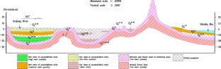
Data availability

The data used to support the fndings of this study are available from the corresponding author upon request.

Abascal E, Gomez-Coma L, Ortiz I, Ortiz A (2022) Global diagnosis of nitrate pollution in groundwater and review of removal technologies. Sci Total Environ 810:152233

Article   CAS   Google Scholar  

Abu-alnaeem M, Yusoff I, Ng T, Alias Y, Raksmey M (2018) Assessment of groundwater salinity and quality in Gaza coastal aquifer, Gaza Strip, Palestine: an integrated statistical, geostatistical and hydrogeochemical approaches study. Sci Total Environ 615:972–989

Bahadoran Z, Mirmiran P, Ghasemi A, Kabir A, Azizi F, Hadaegh F (2015) Is dietary nitrate/nitrite exposure a risk factor for development of thyroid abnormality? A systematic review and meta-analysis. Nitric Oxide 47:65–76

Banyikwa A (2023) Geochemistry and sources of fluoride and nitrate contamination of groundwater in six districts of the Dodoma region in Tanzania. Scient African 21:e01783

Bellettini A, Viero A, Neto A (2019) Hydrochemical and contamination evolution of Rio Bonito aquifer in the carboniferous region, Paraná Basin, Brazil. Environ Earth Sci 78:1–15

Google Scholar  

Bian JM, Zhang ZZ, Han Y (2015) Spatial variability and health risk assessment of nitrogen pollution in groundwater in Songnen Plain. J Chongqing Univer 38(4):104–111 ( (in Chinese with English abstract) )

CAS   Google Scholar  

Bouderbala A (2019) The impact of climate change on groundwater resources in coastal aquifers: case of the alluvial aquifer of Mitidja in Algeria. Environ Earth Sci 78:1–13

Article   Google Scholar  

Canadian Council of Ministers of the Environment (CCME) (2014) Canadian environmental quality guidelines

Fujian Provincial Sports Bureau, China (2022) The fifth National Physical Fitness Monitoring Bulletin of Fujian Province. Fujian Province. (in Chinese)

Gallagher T, Gergel S (2017) Landscape indicators of groundwater nitrate concentrations: an approach for trans-border aquifer monitoring. Ecosphere 8(12):e02047. https://doi.org/10.1002/ecs2.2047

Gutierrez M, Biagioni R, Alarcon-Herrera M, Rivas-Lucero B (2018) An overview of nitrate sources and operating processes in arid and semiarid aquifer systems. Sci Total Environ 624:1513–1522

Heaton T, Stuart M, Sapiano M, Micallef Sultana M (2012) An isotope study of the sources of nitrate in Malta’s groundwater. J Hydrol 414–415:244–254

International Agency for Research on Cancer (IARC) (2022) Agents Classified by the IARC Monographs 1:132

Jiang WJ, Wang GC, Sheng YZ, Zhao D, Liu CL, Guo YH (2016) Enrichment and sources of nitrogen in groundwater in the Turpan-Hami area, Northwestern China. Expo Health 8:389–400

Kong XK, Zhang ZX, Wang P, Wang YY, Zhang ZJ, Han ZT, Ma LS (2022) Transformation of ammonium nitrogen and response characteristics of nitrifying functional genes in tannery sludge contaminated soil. J Groundwater Sci Eng 10(3):223–232

Lahjouj A, Hmaidi A, Bouhafa K (2020) Spatial and statistical assessment of nitrate contamination in groundwater: Case of Sais Basin, Morocco. J Groundwater Sci Eng 8(2):143–157

Li ZH, Zhang YL, Hu B, Wang LJ, Zhu YC, Li JF (2018) Driving action of human activities on NO 3 – -N pollution in confined groundwater of Togtoh County. Inner Mongolia Acta Geoscientica Sinica 39(3):358–364 ( (in Chinese with English abstract) )

Li Y, Kang FX, Zou AD (2019) Isotope analysis of nitrate pollution sources in groundwater of Dong’e geohydrological unit. J Groundwater Sci Eng 7(2):145–154

Li ZH, Li YS, Hao QC, Li JF, Zhu YC (2021) Characteristics, genesis and treatment measures of NO 3 type groundwater in Xiamen, Fujian Province. Geology in China 48(5): 1441–1452. 6 (in Chinese with English abstract)

Menció A, Mas-Pla J, Otero N, Regàs O, Boy-Roura M, Puig R, Bach J, Domènech C, Zamorano M, Brusi D, Folch A (2016) Nitrate pollution in groundwater; all right…, but nothing else? Sci Total Environ 539:241–251

Ministry of Ecology and Environmental PRC (2013) Chinese population Exposure Parameters Manual: Volume for children. Beijing, China Environmental Press (in Chinese).

Ministry of Ecology and Environmental PRC (2013) Chinese population Exposure Parameters Manual: Adult volume. Beijing, China Environmental Press ( in Chinese )

Monteny G (2001) The EU nitrates directive: a european approach to combat water pollution from agriculture. In Optimizing Nitrogen Management in Food and Energy Production and Environmental Pro tection: Proceedings of the 2nd International Nitrogen Conference on Science and Policy. The Scientific World 1(S2) 927–935

Musaed H, Al-Bassam A, Zaidi F, Alfaifi H, Ibrahim E (2020) Hydrochemical assessment of groundwater in mesozoic sedimentary aquifers in an arid region: a case study from Wadi Nisah in Central Saudi Arabia. Environ Earth Sci 79:1–12

National Health Commission, PRC, Standardization Administration, PRC (2022) Standards for dringing water quality. Beijing (in Chinese)

Panneerselvam B, Muniraj K, Duraisamy K, Pande C, Karuppannan S, Thomas M (2023) An integrated approach to explore the suitability of nitrate-contaminated groundwater for drinking purposes in a semiarid region of India. Environ Geochem Health 45:647–663

Papazotos P, Koumantakis I, Vasileiou E (2019) Hydrogeochemical assessment and suitability of groundwater in a typical Mediterranean coastal area: A case study of the Marathon basin, NE Attica, Greece. HydroResearch 2:49–59

Peixoto F, Cavalcante I, Gomes D (2020) Influence of land use and sanitation issues on water quality of an urban aquifer. Water Resour Manage 34:653–674

Pouye A, Cissé Faye S, Diédhiou M, Gaye C, Taylor R (2023) Nitrate contamination of urban groundwater and heavy rainfall: Observations from Dakar. Senegal Vadose Zone Jl 22:e20239

Rahman A, Mondal N, Tiwari K (2021) Anthropogenic nitrate in groundwater and its health risks in the view of background concentration in a semiarid area of Rajasthan. India. Scient Rep 11(1):1–13

Rezende D, Nishi L, Coldebella P, Mantovani D, Soares P, Carlos Valim Junior N, Vieira A, Bergamasco R (2019) Evaluation of the groundwater quality and hydrogeochemistry characterization using multivariate statistics methods: case study of a hydrographic basin in Brazil. Desalin Water Treat 161:203–215

Romanelli A, Soto D, Matiatos I, Martínez D, Esquius S (2020) A biological and nitrate isotopic assessment framework to understand eutrophication in aquatic ecosystems. Sci Total Environ 715:136909

Sheng DR, Wen XH, Feng Q, Wu J, Si JH, Wu M (2019) Groundwater nitrate pollution and human health risk assessment in the Zhangye Basin, Gansu. China J Desert Res 39(5):37–44 ( (in Chinese with English abstract) )

Stuart M, Gooddy D, Bloomfield J, Williams A (2011) A review of the impact of climate change on future nitrate concentrations in groundwater of the UK. Sci Total Environ 409(15):2859–2873

Sun XB, Guo CL, Zhang J, Sun JQ, Cui J, Liu MH (2023) Spatial-temporal difference between nitrate in groundwater and nitrogen in soil based on geostatistical analysis. J Groundwater Sci Eng 11:37–46

Tokazhanov G, Ramazanova E, Hamid S, Bae S, Lee W (2020) Advances in the catalytic reduction of nitrate by metallic catalysts for high efficiency and N 2 selectivity: A review. Chem Eng J 384:123252

United States Environment Protection Agency (U.S. EPA) (2022) Integrated risk information systerm

United States Environmental Protection Agency (U.S. EPA) (2017) Drinking water contaminants–standards and regulations

Verma A, Sharma A, Kumar R, Sharma P (2023) Nitrate contamination in groundwater and associated health risk assessment for Indo-Gangetic Plain. India Groundwater for Sustain Dev 23:100978

Vilmin L, Mogollon J, Beusen A, Bouwman A (2018) Forms and subannual variability of nitrogen and phosphorus loading to global river networks over the 20th century. Global Planet Change 163:67–85

Ward M, Jones R, Brender J, De Kok T, Weyer P, Nolan B, Villanueva C, Van Breda S (2018) Drinking water nitrate and human health: an updated review. Int J Environ Res Public Health 15(7):1557

WHO (2017) Guidelines for Drinking Water Quality: Fourth Edition Incorporating the First Addendum, fourthed. World Health Organization, Geneva

Yang M, Fei YH, Ju YW, Ma Z, Li HQ (2012) Health risk assessment of groundwater Pollution- a case study of typical city in North China Plain. J Earth Sci 23(3):335–348

Zakaria N, Gibrilla A, Owusu-Nimo O, Adomako D, Anornu G, Fianko J, Gyamfi C (2023) Quantifcation of nitrate contamination sources in groundwater from the Anayari catchment using major ions, stable isotopes, and Bayesian mixing model. Ghana Environ Earth Sci 82:381

Download references

Acknowledgements

This work was supported by the China Geological Survey project (Nos. DD20190303, DD20221773, DD20230459) and Zhejiang Provincial Geological Special Fund Project (No. 2023010)

Author information

Authors and affiliations.

Fujian Provincial Key Laboratory of Water Cycling and Eco-Geological Processes, Xiamen, 361000, China

Zhenghong Li, Jianfeng Li & Yasong Li

Institute of Hydrogeology and Environmental Geology, Chinese Academy of Geological Sciences, Shijiazhuang, 050061, China

Zhejiang Institute of Geosciences, Hangzhou, 310007, China

Jin’ou Huang

You can also search for this author in PubMed   Google Scholar

Contributions

Writing-original draft, Zhenghong Li; Reviewing and editing, Jianfeng Li, Yasong Li; Methodology, Jianfeng Li, Yasong Li, Zhenghong Li, Jin’ou Huang; Investigation, data collection, Zhenghong Li, Jianfeng Li; Figures preparation, Zhenghong Li, Jin’ou Huang; All authors have read and agreed to the submitted version of the manuscript.

Corresponding author

Correspondence to Jianfeng Li .

Ethics declarations

Conflict of interest.

The authors have no relevant financial or non-financial interests to disclose.

Additional information

Publisher's note.

Springer Nature remains neutral with regard to jurisdictional claims in published maps and institutional affiliations.

Rights and permissions

Springer Nature or its licensor (e.g. a society or other partner) holds exclusive rights to this article under a publishing agreement with the author(s) or other rightsholder(s); author self-archiving of the accepted manuscript version of this article is solely governed by the terms of such publishing agreement and applicable law.

Reprints and permissions

About this article

Li, Z., Li, J., Huang, J. et al. Nitrate contamination in groundwater and its health risk assessment: a case study of Quanzhou, a typical coastal city in Southeast China. Environ Earth Sci 83 , 331 (2024). https://doi.org/10.1007/s12665-024-11608-z

Download citation

Received : 21 December 2023

Accepted : 18 April 2024

Published : 13 May 2024

DOI : https://doi.org/10.1007/s12665-024-11608-z

Share this article

Anyone you share the following link with will be able to read this content:

Sorry, a shareable link is not currently available for this article.

Provided by the Springer Nature SharedIt content-sharing initiative

• Spatial distribution
• NO 3 − type water
• Hydrochemistry
• Risk assessment
• Southeast coast
• Find a journal
• Publish with us
• Track your research

• Open access
• Published: 11 May 2024

Biological response to Przewalski’s horse reintroduction in native desert grasslands: a case study on the spatial analysis of ticks

• Yu Zhang 1   na1 ,
• Jiawei Liu 1   na1 ,
• Ke Zhang 2 ,
• Anqi Wang 1 ,
• Duishan Sailikebieke 3 ,
• Zexin Zhang 4 ,
• Tegen Ao 5 ,
• Liping Yan 1 ,
• Dong Zhang 1 ,
• Kai Li 1 &
• Heqing Huang 6  

BMC Ecology and Evolution volume  24 , Article number:  61 ( 2024 ) Cite this article

117 Accesses

1 Altmetric

Metrics details

Reintroduction represents an effective strategy for the conservation of endangered wildlife, yet it might inadvertently impact the native ecosystems. This investigation assesses the impact of reintroducing endangered Przewalski's horses into the desert grassland ecosystem of the Kalamaili Nature Reserve (KNR), particularly its effect on the spatial distribution of ticks. In a 25 km 2 core area of Przewalski's horse distribution, we set up 441 tick sampling sites across diverse habitats, including water sources, donkey trails, and grasslands, recording horse feces and characteristics to analyze the occurrence rate of ticks. Additionally, we gathered the data of 669 fresh feces of horses. To evaluate the spatial dynamics between these feces and ticks, we used methods such as Fixed Kernel Estimation (FKE), Moran’s I spatial autocorrelation index, and Generalized Linear Models (GLM).

The dominant species of ticks collected in the core area were adult Hyalomma asiaticum (91.36%). Their occurrence rate was higher near donkey trails (65.99%) and water sources (55.81%), particularly in areas with the fresh feces of Przewalski's horses. The ticks’ three risk areas, as defined by FKE, showed significant overlap and positive correlation with the distribution of Przewalski's horses, with respective overlap rates being 90.25% in high risk, 33.79% in medium risk, and 23.09% in low risk areas. Moran's I analysis revealed a clustering trend of the fresh feces of Przewalski's horses in these areas. The GLM confirmed a positive correlation between the distribution of H. asiaticum and the presence of horse fresh feces, alongside a negative correlation with the proximity to water sources and donkey trails.

Conclusions

This study reveals the strong spatial correlation between Przewalski's horses and H. asiaticum in desert grasslands, underlining the need to consider interspecific interactions in wildlife reintroductions. The findings are crucial for shaping effective strategies of wildlife conservation and maintaining ecological balance.

Peer Review reports

Desert grassland ecosystems are a critical component of terrestrial ecosystems, harboring unique communities of flora and fauna adapted to extreme arid conditions [ 1 , 2 ]. Nonetheless, the ungulates in these ecosystems, serving as pivotal species for maintaining ecological balance, are confronting a series of challenges including habitat loss and climate change [ 3 , 4 ]. In this context, endangered species reintroduction stands as one of the effective measures for the restoration and preservation of desert grassland ecosystems, as well as for augmenting their biodiversity [ 2 , 5 , 6 ]. The successful reintroduction of the Przewalski’s horse into the Kalamaili Nature Reserve (KNR) in Xinjiang, China, serves as a quintessential example of this practice [ 7 , 8 ]. The KNR is located at the southern edge of the Junggar Basin in northwestern China, characterized by an arid climate and infrequent rainfall, leading to the formation of a unique Central Asian continental desert grassland biota [ 8 , 9 ]. Since 2001, the population of Przewalski's horses in the region has experienced substantial growth, escalating from 27 to 230 by the year 2019 [ 8 , 9 , 10 ]. This resurgence of this population in the KNR provides us with a unique opportunity to explore the responses of related species following the reintroduction of large ungulates into their native ecosystems.

However, as an introduced species, the reintroduction of Przewalski's horses could potentially give rise to some unforeseen ecological consequences, especially regarding the impact on parasite dynamics [ 10 , 11 , 12 ]. In response, a specialized team undertakes annual monitoring of parasitic diseases within the Przewalski’s horses [ 10 , 12 , 13 , 14 ]. It was discovered that the Przewalski's horses in the KNR are heavily infected with the obligate parasite, Gasterophilus spp. [ 10 , 14 ], with infection intensity more than double that found in the sympatric Mongolian wild ass ( E. hemionus ) [ 13 ]. The research team initially aimed to study the transmission patterns of the myiasis disease by tracking and examining the feces of Przewalski's horses, as the larvae of these Gasterophilus spp. tend to burrow into the soil within 5 min after the horse's defecation [ 10 , 11 , 12 , 13 , 14 ]. However, in recent investigations, we inadvertently found that ticks frequently appeared near the feces of the Przewalski's horses, which sparked our interest in studying the spatial distribution relationship between Przewalski's horses’ feces and ticks. Additionally, during the peak season of tick activity in spring and summer [ 15 , 16 ], we incidentally discovered the Hyalomma asiaticum (Acari: Ixodidae) parasitizing on the abdomen of deceased Przewalski's horses (Fig. S1), and also fortuitously encountered naturally detached and engorged adult H. asiaticum near the Przewalski's horse dung piles (Fig. S2). These observations not only corroborate the hypothesis that Przewalski's horses could serve as potential new hosts for H. asiaticum but also provide important clues into the interactions between hosts and parasites in the KNR.

H. asiaticum , a tick prevalent in arid desert regions, poses a direct threat to host animals through biting, leading to conditions such as inflammation and anemia [ 17 , 18 , 19 , 20 ]. It also plays a crucial role in the transmission of various diseases, including Crimean-Congo Hemorrhagic Fever (also known as Xinjiang Hemorrhagic Fever locally) and Rickettsial diseases, among others [ 21 , 22 ]. Being a three-host parasitic tick, H. asiaticum progresses through a life cycle consisting of four stages: egg, larva, nymph, and adult [ 15 ]. Parasitism occurs in the stages after the egg, with immature H. asiaticum ticks predominantly parasitizing small rodents, and adults typically attaching to large ungulates such as horses, cattle, and sheep [ 23 , 24 , 25 , 26 , 27 ]. Ticks generally employ two strategies to seek hosts: the ambush strategy and the hunter strategy. In the ambush strategy, ticks usually position themselves on the top of plants or rocks, waiting for hosts to pass by. Conversely, in the hunter strategy, ticks move through the environment, actively seeking out hosts by detecting carbon dioxide released by the hosts and following trails of the hosts’ excreta [ 28 , 29 ]. H. asiaticum are typical hunter type ticks, as they conceal themselves in the surrounding environment and actively wait to attack passing hosts [ 15 , 28 , 30 ]. Notably, the adult H. asiaticum in the unfed state, while actively seeking host animals, not only demonstrate a strong preference towards large ungulate hosts but also amplify the risk of disease transmission during this process [ 15 , 18 ]. Hence, understanding and monitoring the distribution of ticks at this specific life stage is paramount for the efficacious prevention and management of the pervasive transmission of tick-borne diseases in the KNR.

The water sources in arid and desert regions, along with their adjacent areas, are vital habitats for wildlife [ 31 , 32 ]. In the KNR, the Przewalski's horses exhibit unique seasonal behaviors. In the spring and summer, they frequently travel along designated paths, known as 'donkey trails' [ 11 ], to reach water sources. They tend to congregate around these water sources and the adjacent grasslands, showing a pronounced propensity to cluster more notably than other ungulate species such as the Mongolian wild ass ( E. hemionus ) and the Goose-throated gazelle ( Gazella subgutturosa ) [ 7 , 11 , 33 ]. This behavioral pattern does not only highlight the attraction of water sources for Przewalski’s horses but also presents potential opportunities for the local parasite populations to spread [ 11 , 12 ]. Although there is a notable correlation between the spatial distribution of wildlife and parasites [ 11 , 12 , 29 , 34 , 35 ], studies specifically examined the relationship between the distribution of Przewalski’s horses and parasites are comparatively limited [ 11 , 12 ]. A previous study revealed that areas within a 300 m radius surrounding water sources, nortably high density of Przewalski's horse feces were observed [ 11 ]. Furthermore, there is a positive correlation between the density of Przewalski's horse feces and the spatial distribution of the Gasterophilus spp. [ 11 , 12 ]. This further confirms the significance of water sources and their surrounding areas as principal locales for the interaction between Przewalski's horses and potential parasites. Moreover, a prior report indicated that before the reintroduction of Przewalski's horses into the KNR, large-scale tick infestations were not observed [ 16 ]. However, this historical absence of infestations does not rule out the potential for these horses to experience health challenges when reintroduced, as they may lack natural immunity or the ability to adapt to local parasites [ 11 , 12 , 13 ]. For instance, a decade after elk ( Cervus canadensis ) were reintroduced to southeastern Kentucky, USA, the distribution of local ticks became more widespread [ 36 ]. Similarly, in Japan, as populations of sika deer ( C. nippon ) and wild boar ( Sus scrofa ) increased, the distribution of the Haemaphysalis ticks changed, potentially increasing the transmission of the pathogen causing tick-borne diseases [ 37 ]. These findings highlight the importance of monitoring changes in local ticks distribution following reintroduction of wildlife [ 38 , 39 ]. Therefore, this study focused on the Przewalski's horses and the ticks, conducted systematic surveys of typical habitats for horses in the KNR, including water sources, grasslands, and donkey trails. It incorporates the activity patterns of Przewalski's horses to thoroughly examine the spatial distribution relationship between host and parasite. The study aims to analyze the risk areas of ticks in the core distribution areas of Przewalski's horses. This study will provide a comprehensive assessment of whether reintroduced animals have expanded the distribution range of parasites, thereby offering a new perspective on understanding the synergistic adaptation of reintroduced species with related species in their new environment.

Research area

The KNR (88°30’ ~ 90°03’E, 40°36’ ~ 46°00’N) is located in the Junggar Basin of Xinjiang, China (Fig.  1 ), and is a typical arid and semi-arid desert grassland. The reserve has scarce water resources, with an annual precipitation of only about 159 mm [ 10 , 40 ]. The composition of plant communities is relatively simple, featuring an average coverage of 20 to 30%, primarily consisting of xerophytic shrubs and herbs, such as Ceratoides spp., Tamarix spp., Haloxylon spp., Anabasis spp., and Reaumuria spp. [ 40 ]. Among them, the Hong Liu, Xiao, No.6 are key water sources within the region [ 11 , 12 ]. Przewalski’s horses primarily depend on these water sources for their distribution, whereas other wildlife, including the E. hemionus and the G. subgutturosa , have a broad distribution throughout the entire reserve [ 7 , 12 , 31 , 40 ]. Based on this context, this study was conducted during the season when is the peak of H. asiaticum activity from April to June 2021 [ 20 , 41 ], focusing primarily on the spatial utilization patterns of Przewalski’s horses and their impact on the distribution of ticks. The research was centered around three water sources, designating a 25 km 2 area as the study area, which also constitutes the core habitat of Przewalski’s horses (Fig.  1 ).

Tick sampling sites in Kalamaili Nature Reserve (KNR). Note: The left section delineates the three types of study habitats, namely, donkey trails, water sources, and grasslands; the center displays the distribution map of the sampling sites of ticks; the right section represents the study area

Research method

Ticks sampling sites’ survey.

Tick sampling sites were set up across three types of typical habitats: water sources, donkey trails, and grasslands, and the specific sampling method is shown in Fig. S3. In each habitat, based on the frequency of Przewalski’s horses’ activities, three types of dung piles were randomly selected for tick collection: stallion feces, non-stallion feces and no feces (Fig. S4). Stallion feces are generally higher than the feces of non-stallions because stallions repeatedly defecate in the same location, forming larger mounds. Conversely, non-stallion defecation behavior tends to be more random, usually occurring just once at various locations, resulting in smaller dung piles.

Arid desert regions are mainly covered with small shrubs. In such environments, ticks typically adopt an active waiting and attacking strategy for survival [ 28 , 30 ].

Therefore, to ensure consistency in the sampling process, we limited time at each tick sampling site to 5 min, employing the 'waiting for ticks' method as referenced by Yu et al. [ 16 ]. The specific procedure involved shaking the ground with sticks in areas with Tamarix spp. and Haloxylon spp. to attract and collect non-engorged ticks [ 16 , 28 , 30 ]. Concurrently, each sampling site was centered within a defined area of 2 m × 2 m, thereby maintaining an effective sampling area of 4 m 2 . Using the “Create Buffer” and “Create Fishnet Tool” in ArcGIS 10.3, buffer zones were delineated, extending 100 m from the three water sources perimeters and 10 m along the donkey trails. Additionally, the grassland area was segmented into a grid pattern, each cell measuring 500 m × 500 m. The collected data were stored in KML format and subsequently imported into a GPS device (eTrex309x, Garmin Ltd., Olathe) to precisely locate the sampling sites for efficient field collection. Furthermore, at the sampling sites where dung piles were present, we conducted detailed measurements of each dung pile’s characteristics. The dimensions of the dung piles (length × width × height in cm) were recorded using a tape measure. The moisture content of these dung piles was assessed using a soil moisture meter (PR-ECTH-SC-37DC, Pruisen brand Ltd., China) with an accuracy of ± 2% RH. Based on these readings, moisture levels were classified into two categories: low moisture (0 ~ 15% RH) and high moisture (15 ~ 30%RH). This classification approach is based on previous experience and is consistent with the fecal moisture classification standards found in the literature [ 42 , 43 ].

The classification and identification of the ticks, along with the tallying of their numbers and other pertinent details, were carried out in the laboratory. Using a SZ51 stereomicroscope equipped with LED lighting / SZ2-ILST (Olympus corporation, Tokyo, Japan), we scrutinized the distinguishing features of the ticks, which encompassed the dorsal surface, ventral surface, eye, basis capituli, scutum, porose area, spiracle plate, marginal groove, and genital groove [ 44 , 45 , 46 ].

Przewalski’s horses’ spatial distribution survey

The distribution and density of wildlife feces are reliable indicators of spatial utilization in designated areas [ 40 , 47 , 48 ]. For data collection, we tracked Przewalski’s horses, and recorded the GPS coordinates of fresh feces after the horses had departed from the area. Our survey encompassed 8 herds, comprising a total of 60 reintroduced horses [ 12 ]. The study area included frequently visited water sources and grasslands in the KNR, enveloping the same 20km 2 area also surveyed for ticks [ 12 ].

Data analysis

The occurrence rate of h. asiaticum under different conditions.

Formula ( 1 ), \({P}_{ij}\) represents the occurrence rate of ticks under different conditions, \({N}_{ij}\) is the number of sampling sites with ticks under different conditions, \({M}_{ij}\) is the total number of sampling sites under different conditions. \(i\) is water source, donkey trail, grassland, and \(j\) is stallion-feces, non-stallion-feces and no-feces.

Analysis of H. asiaticum occurrence rate and Przewalski’s Horse Dung Parameters

Given the observed higher occurrence rates of H. asiaticum near the dung piles of Przewalski’s horses, this study investigates the influence of the dung piles’ physical characteristics (size and moisture) on the occurrence rate of the H. asiaticum . Dung pile size parameters include three key dimensions: pile height (cm), bottom area (cm 2 ), and volume (cm 3 ). Concurrently, the moisture content of the dung piles is categorized into two levels: low moisture (0 ~ 15% RH) and high moisture (15 ~ 30%RH). For maintaining consistency and ensuring comparability among variables, the variables were standardized using the Z-score function from the R package scale. The relationship between the number of the H. asiaticum and dung pile size was analyzed through Pearson correlation analysis. A correlation coefficient (r) approaching 1 indicates a stronger correlation. T-tests were used to compare the size differences of dung piles with and without the presence of the H. asiaticum , using p  < 0.05*, p  < 0.01**, and p  < 0.001*** as thresholds to ascertain the levels of statistical significance. By calculating the occurrence rates of the H. asiaticum at different moisture levels, this study visually presents the results using bar graphs. The plotting was conducted utilizing the ‘ggplot2’ package in R.

Risk area analysis of the H. asiaticum

Based on the analysis results from the occurrence rates of the H. asiaticum , this study selected the GPS locations where the H. asiaticum was found. Additionally, by referencing to the GPS locations of Przewalski’s horses fresh dung piles reported in Zhang et al. [ 12 ], a comprehensive assessment of the spatial distribution relationship between the H. asiaticum and the horse fresh feces. These data underwent preprocessing using the R packages ‘sp’, ‘sf’, and ‘tidyverse’, which included data cleaning and standardization to ensure accuracy and consistency. The R package ‘adehabitatHR’ was utilized to calculate the 95% Minimum Convex Polygon (MCP) for the fresh feces of Przewalski’s horses, establishing their distribution within the 25 km 2 study area (Formula 2 ). The definition of risk areas is based on Fixed Kernel Estimation (FKE) to categorize the distribution of ticks into high, medium, and low risk levels. Specifically, 50% FKE is used to define high risk areas, 75% FKE for medium risk areas, and 95% FKE for low risk areas (Formula 3 ). This classification reflects the occurrence rate of H. asiaticum within the study area. The Intersect module in the Arctoolbox of ArcGIS 10.3 software was employed to evaluate the spatial overlap between the distribution of Przewalski’s horses and the three risk areas of the H. asiaticum .

MCP calculation formula:

Formula ( 2 ), S is the area, and \({x}_{i}\) and \({y}_{i}\) are the latitude and longitude.

FKE calculation formula:

Formula ( 3 ), n represents the number of ticks, h is the bandwidth, and \({dist}_{i}\) represents the distance between the point i and the geographical coordinates.

Spatial autocorrelation analysis

Drawing from the findings of the risk area analysis of the H. asiaticum , this study conducted a bivariate spatial autocorrelation analysis of the spatial distribution of horse fresh feces within the three risk areas. We employed the nearest neighbor method to create spatial weight matrices and used these matrices to calculate the Cross Moran’s I index for each area [ 49 , 50 ]. This index aims to evaluate the degree of clustering between the horse fresh feces and the risk distribution areas of the H. asiaticum . Specifically, the Moran’s I value approaching 1 indicates a high level of clustering of horse fresh feces in the area, while values close to 0 suggest a weaker spatial association with horse fresh feces.

Kernel density estimation and multiscale correlation analysis

The spatial density of the Przewalski’s horse fresh feces and the H. asiaticum was calculated using Kernel Density Estimation (KDE) in the Spatial Analyst module of ArcGIS 10.3 (Formula 4 ). In this study, a uniform pixel value of 20 and a search radius of 500 m [ 12 ], were configured to precisely evaluate the correlation between the Przewalski’s horse fresh feces and the H. asiaticum across multiple scales. Five scales, 100 m, 250 m, 500 m, 750 m, and 1000 m (Fig. S5), were selected for conducting Pearson correlation analysis. We used ArcGIS 10.3 to construct grids corresponding to the five scales and to generate a central representative point for each grid. Based on the KDE layers of the H. asiaticum and Przewalski’s horse fresh feces, we extracted the raster attribute values for each point at every scale. The three risk areas of tick distribution were used as a backdrop for intersection processing. Ultimately, the ‘cor’ function in R was applied to perform Pearson correlation analysis between the attribute values of the H. asiaticum and the fresh feces from Przewalski’s horses at each scale within each risk area.

KDE calculation formula:

In formula ( 4 ), R represents the search radius, \({pop}_{i}\) represents the number of ticks or horses’ fresh feces at point i, and \({dist}_{i}\) represents the distance between the point i and the geographical coordinates.

Generalized linear model analysis

Based on the results of multiscale correlation analysis, this study selected the 100 m scale and used the Generalized Linear Model (GLM) to accurately evaluate the impact of Przewalski’s horses and external environmental factors on the H. asiaticum . Using the nearest neighbor analysis tool in ArcGIS 10.3, we conducted nearest neighbor analysis on the three water sources and donkey trails. This analysis facilitated the identification of two crucial parameters: the nearest distance to water sources and the nearest distance to donkey trails. Before constructing the GLM, to ensure the model's accuracy and stability, we conducted multicollinearity diagnostics using the Variance Inflation Factor (VIF). The VIF for each explanatory variable was calculated using the 'car' package in R. If VIF ≥ 5, variables were excluded from the model. By constructing a GLM model with the ‘glm’ function in R, we set the attribute values of the H. asiaticum at the 100 m scale as the response variable, while considering the attribute values of fresh feces of Przewalski’s horses, the nearest distance to water sources, and the nearest distance to donkey trails as explanatory variables.

The ticks sampling sites survey results

During the peak period of ticks, this study encompassed 441sampling sites. Among these, the 219 sampling sites (49.66%) found unfed state adult ticks. A cumulative count of 301 host-seeking ticks was collected, with 275 being H. asiaticum (91.36%),identified across all 219 sites. In addition, 14 Dcrmacentor nuttalli were collected from 4 sampling sites (4.65%), and 12 Rhipicephalus microplus were found across 3 sampling sites (3.99%). The detailed statistics regarding species identification and distribution are presented in Table S1.

The occurrence rate of H. asiaticum

Given that H. asiaticum is the predominant species in this region and is present at all tick sampling sites, this study conducted an in-depth analysis of the spatial distribution of the H. asiaticum . The occurrence rates of the H. asiaticum under different habitats are as follows: donkey trail (65.99%) > water source (55.81%) > grassland (39.04%). Moreover, regions with a high frequency of Przewalski’s horse distribution also exhibit elevated occurrence rates of H. asiaticum , characterized by the following sequence: stallion-feces (70.06%) > non-stallion-feces (51.67%) > no-feces (25.97%). In the following sites, the occurrence rate of H. asiaticum exceeded 50%: stallion feces at water source (77.27%) > stallion feces at donkey trail (72.88%) > non-stallion feces at grassland (53.41%) > stallion feces at grassland (51.85%) > non-stallion feces at donkey trail (50.00%) (Table  1 ).

H. asiaticum occurrence rate and Przewalski’s horse dung parameters

Pearson correlation analysis demonstrated a positive correlation between the size of Przewalski’s horse feces and the number of the H. asiaticum . The correlation coefficients are as follows: fecal height ( r (287)  = 0.401, P  < 0.001), fecal bottom area ( r (287)  = 0.328, P  < 0.001), fecal volume ( r (287)  = 0.369, P  < 0.001). The T-test analysis revealed that the H. asiaticum prefer to conceal themselves near larger piles of Przewalski’s horse feces (Fig.  2 ). Specifically, stallion feces showed significant differences in the height (t (167)  = 3.659, P  < 0.001), bottom area (t (167)  = 2.752, P  < 0.001), and volume (t (167)  = 3.846, P  < 0.001), while non-stallion-feces only showed significant difference in height (t (120)  = 3.000, P  < 0.01).

The T-test analysis of Przewalski's horses fecal size differences in presence and absence of H. asiaticum

The study found that the fresher the Przewalski’s horse feces, the higher the occurrence rate of the H. asiaticum , and the occurrence rates of ticks near stallion feces is generally higher than near non-stallion feces (Fig.  3 ). The occurrence rates of the H. asiaticum was distributed as follows: high humidity of stallion feces (94.29%) > high humidity of non-stallion feces (77.27%) > low humidity of stallion feces (63.64%) > low humidity of non-stallion feces (45.92%).

The correlation between humidity of Przewalski's horse feces and the occurrence rate of H. asiaticum

Three risk area of H. asiaticum

This analysis used the data from 219 sampling sites of ticks and the 669 locations of Przewalski's horse fresh feces. (Fig.  4 a, b). The area covered by fresh feces from Przewalski's horses in the survey region was determined to be 14.31 km 2 , as calculated by the 95% MCP method (Fig.  4 a). We categorized the risk areas for H. asiaticum into high, medium, and low categories based on 50% FKE, 75% FKE, and 95% FKE thresholds. Subsequent analysis revealed a positive correlation between the risk levels of ticks and the overlap rate with the distribution of Przewalski's horse (Table  2 ). Specifically, the high-risk area for H. asiaticum was 8.00 km 2 , of which 90.25% overlapped with the distribution of Przewalski's horses, covering an area of 7.22 km 2 (Fig.  4 b, Table  2 ); the medium-risk area was 7.04 km 2 , with 33.79% overlap rate, overlap area covering 4.80 km 2 (Fig.  4 b, Table  2 ); and the low-risk area was 9.96 km 2 , with 23.09% overlap rate, overlap area covering 2.30 km 2 (Fig.  4 b, Table  2 ).

Distribution of Przewalski’s horse fresh feces and H. asiaticum . a Distribution area of Przewalski’s horse fresh feces. b Three risk areas of H. asiaticum . c Kernel Density Estimation (KDE) distribution of fresh feces from Przewalski’s horses. d KDE distribution of H. asiaticum

Spatial autocorrelation index Moran's I of H. asiaticum and Przewalski's horse fresh feces

In the three designated risk areas, we observed that the distribution of H. asiaticum and horse fresh feces exhibited an extremely high degree of spatial autocorrelation, with Moran's I values approaching 1 (Table  3 ). The Z-score values further substantiated the statistical significance of this aggregation pattern, thereby greatly diminishing the probability of a random distribution ( P  < 0.001). In the high-risk area, Moran's I value was 0.998 (Z = 16.499, P  < 0.001) and similarly, in the medium-risk area, Moran's I was also 0.998 (Z = 8.968, P  < 0.001). This indicates a very strong spatial clustering of H. asiaticum and horse fresh feces in both high and medium-risk areas. In the low-risk area, the Moran's I value was slightly lower at 0.994 (Z = 8.335, P  < 0.001), still indicating a significant spatial aggregation trend of H. asiaticum and horse fresh feces (Table  3 ).

Kernel density estimation and multiscale correlation analysis of H. asiaticum and Przewalski's horse fresh feces

The KDE analysis indicated that the distribution of fresh feces from Przewalski's horses is predominantly concentrated to the north of major water sources, including HongLiu and No. 6 (Fig.  4 c). Similarly, H. asiaticum were also predominantly found in the areas near these water sources (Fig.  4 d). To quantify the correlation between H. asiaticum and horse fresh feces at different scales, this study conducted Pearson correlation analysis at distances at distances of 100 m, 250 m, 500 m, 750 m, and 1000 m (Table  4 ). The specific distribution sites at these five scales are presented in Fig. S5. At the 100 m scale, a positive correlated was observed across all risk areas, with the strength of the correlation diminishing in the order of high, medium, and low. This suggests that the presence of horse fresh feces may be more closely correlation with the distribution of H. asiaticum at smaller spatial scales. However, at larger scales such as 500 m, 750 m, and 1000 m, the variability in correlations indicates that factors other than horse fresh feces could be influencing the distribution of H. asiaticum , particularly noted in the negative correlations observed in medium-risk areas at 500 m and 1000 m scales (Table  4 ).

Comprehensive analysis using generalized linear model

In this study, we used a GLM to unveil the significant correlations between the distribution of H. asiaticum and three pivotal factors: the distribution of the horse fresh feces; nearest distance to water sources; nearest distance to donkey trails (Table  5 ). The multicollinearity analysis results show that the VIF for the horse fresh feces is 1.134, for the nearest distance to water sources is 1.048, and for the nearest distance to donkey trails is 1.143. The VIF values of these three variables are close to 1, indicating almost no linear correlation between them, making them suitable as explanatory variables in the GLM. The intercept of the GLM is 13.536 (T = 44.170, P  < 0.001). Notably, the distribution of fresh feces from Przewalski’s horses showed a significant positive correlation with the distribution of H. asiaticum (T = 27.980, P  < 0.001), suggesting that accumulations of horse feces can attract the ticks. Conversely, the proximity to water sources exhibited a negative correlation with the tick distribution (T = -14.940, P  < 0.001), similar to the proximity to donkey trails (T = -25.630, P  < 0.001), indicating that closer proximity to water sources and donkey trails increases the likelihood of encountering H. asiaticum (Table  5 ).

This study aims to delve into the impact of the reintroduction of Przewalski’s horses on the parasites in the desert grassland ecosystem of the KNR, with a focus on analyzing the influence of their distribution patterns on H. asiaticum . The reintroduction of Przewalski’s horses, an endangered species, not only represents a crucial measure for biodiversity conservation but also significantly affects the structure of the local parasitic community, which has been confirmed by previous studies [ 10 , 11 , 12 ]. Although the primary intent of reintroduction is to protect or restore ecosystems, it may result in unintended consequences [ 38 , 39 , 51 ]. This study is the first to identify a positive correlation between the distribution of Przewalski’s horse feces and the spatial distribution patterns of the H. asiaticum , providing new insights into the mechanisms by which the reintroduction of Przewalski’s horses impacts the parasites in desert grassland ecosystems. This finding is consistent with studies from other regions regarding the relationship between reintroduced species and ticks. For example, in Kentucky, reintroduced elk have turned into hosts for various ticks, potentially expanding their distribution [ 36 ]. Similarly, in Japan, an increase in the population of wildlife has coincided with an increase of ticks [ 37 ]. Therefore, this study points out that even introducing animals for conservation purposes could inadvertently facilitate the spread of ticks and their pathogen carriers [ 36 , 37 ].

The occurrence rates of the H. asiaticum and its relationship with Przewalski’s horse feces constitute the central focus of this study. Previous research has revealed that host feces significantly impact the spatial distribution of parasites [ 12 , 52 , 53 ], evidenced by the parasites’ inclination to gather in the areas proximate to the host’s feces [ 11 , 12 , 15 ]. In light of this context, and considering the tendency of Przewalski’s horses in the KNR to congregate in family units [ 7 , 12 , 54 ], as well as the proactive host-seeking behavior of H. asiaticum [ 15 ], this study posits that zones where Przewalski’s horses frequently defecate are more likely to encounter ticks in an unfed state. This hypothesis was supported by field data indicating that the H. asiaticum was found significantly more frequently in proximity to the Przewalski’s horse feces than in areas without feces. Subsequent analysis elucidated a positive correlation between the size and freshness of the horse feces and the occurrence rates of the H. asiaticum . This phenomenon suggests that Przewalski’s horse feces may provide an important survival environment for the H. asiaticum [ 55 , 56 ]. Significantly, this spatial association is not limited to the H. asiaticum , other studies have also shown that zones of frequent defecation by Przewalski’s horses are considered high-risk for obligate parasites such as horse stomach flies [ 10 , 11 , 12 ]. These findings highlight the necessity of integrating a comprehensive consideration of the multifaceted impacts of reintroducing endangered species on other species within local ecosystems when formulating biodiversity conservation strategies and ecosystem management measures.

In ecological research, animal feces are considered a valuable ecological indicator for discerning their behavioral patterns and spatial distribution [ 47 , 48 ]. Previous studies have confirmed a substantial correlation between the distribution of ungulates and ticks, as exemplified by the findings of Qviller et al. [ 47 ], who discovered a tight spatial association between the distribution of the red deer and the Ixodes ricinis in Norway. Similarly, Schulze et al. [ 57 ] observed a close relationship between the distribution of the white-tailed deer and the Amblyomus ticks in America. However, due to the numerous challenges of field surveys and the limitations in data collection, this study prefers to use fresh feces as an indirect indicator of Przewalski's horses’ activity range. The H. asiaticum , an ectoparasite that actively seeks hosts based on host scent [ 15 , 28 , 30 ], examining the distribution of Przewalski's horse fecal feces can better illustrate the spatial correlation between the host animals and ticks. Furthermore, initial investigations in this study found a relatively high prevalence of ticks near fresh feces of Przewalski's horses, confirming that data on fresh feces from synchronized surveys can serve as an indirect indicator of the spatial association between Przewalski's horses and the H. asiaticum.

Przewalski's horses have a social structure based on family groups, typically consisting of one stallion, three to four mares, and their foals [ 9 , 58 ]. Different genders of Przewalski's horses may display unique activity patterns and territorial marking behaviors, leading to their feces containing different chemical information [ 32 , 43 , 59 ], which could affect their attractiveness to ticks and influence tick distribution. In this study, fecal samples were differentiated by observing that stallions and non-stallions defecate in different locations. Specifically, mares and foals tend to defecate randomly on grasslands, whereas stallions prefer to repeatedly defecate in the central areas of their family group’s territory [ 54 , 58 ]. The results showed a higher probability of ticks near stallion feces than feces of the non-stallions, with the larger feces showing a higher occurrence rate of ticks. This suggests that the spatial distribution of ticks in this region may be related to the volume of Przewalski's horse feces and their gender-specific behaviors.

This finding provides a basis for future research on how gender difference in Przewalski's horses could influence tick distribution. Moreover, the widespread E. hemionus and G. subgutturosa in the reserve exhibit a more dispersed distribution due to their lower dependency on water and higher alertness, leading to the observation of typically drier feces [ 60 , 61 ], which are less suitable for tick spatial distribution studies. According to Zhang et al. [ 12 ] and Huang et al. [ 11 ], fresh feces of these species are rare in our study area, thus their direct impact on the study results is limited. This supports the study's focus on Przewalski's horses, an endangered reintroduced species, and largely excludes the impact of other local wildlife in the study area on the spatial distribution of ticks.

Before the reintroduction of the Przewalski’s horses, the KNR had not shown a high correlation between the distribution of ungulates and ticks [ 16 ]. Research suggests that post-reintroduction, the increased density of host feces from Przewalski's horses may have amplified the spread and reproduction of parasite populations, thereby accelerated the transmission patterns of parasites and potentially altered the ecological chain relationships between local hosts and parasites [ 12 ]. Therefore, this research focuses on analyzing the distribution relationship between the Przewalski's horses and the H. asiaticum , and it quantifies the risk levels of H. asiaticum in the surveyed area. The MCP algorithm was deployed to estimate the distribution area of Przewalski's horses. Although a 100% MCP can include all GPS sites, it may overestimate the area due to extreme points [ 62 ]. Consequently, a 95% MCP was chosen to exclude the impact of extreme points. This method is in line with methods previously employed by researchers to determine the home range of Przewalski's horses [ 7 , 62 ]. The FKE method enhances the MCP by smoothing the distribution area calculation through correcting extreme points [ 12 , 63 ] For this study, 50% FKE, 75% FKE, and 95% FKE were utilized as thresholds to delineate high, medium, and low-risk areas, respectively, in order to quantify the risk areas of the H. asiaticum . Through analysis of the overlap rates, it was observed that areas with the fresh feces form the Przewalski's horses overlap with high-risk areas for the H. asiaticum by more than 90%. This suggests that Przewalski's horses are consistently exposed to tick-infested environments within their activity areas. Moreover, high-risk areas frequently correspond with areas where Przewalski's horses are commonly active and defecate, which aligns with our conclusions drawn from spatial autocorrelation analysis. These methods of analysis approaches allow us to reveal the spatial relationship between the distribution of the H. asiaticum and horse fresh feces, indicating that the tick distribution is not random but closely related to the spatial distribution of horse fresh feces.

The water sources and grasslands are crucial factors for the survival of ungulate species in arid and desert regions [ 31 , 40 ]. The strong reliance of Przewalski’s horses on these water sources often directs their frequent use of donkey trails near these areas, consequently resulting in more severe occurrences of the H. asiaticum in such areas [ 11 , 12 , 31 ]. Grassland areas, being vital habitats for wild ungulates, may exhibit a comparatively lower presence of ticks. This phenomenon could be due to Przewalski’s horses lingering and being active over extended periods in these areas [ 32 ], leading to a higher number of the H. asiaticum successfully attaching to the horses. Therefore, by focusing the analysis on three factors associated with a higher occurrence rate of ticks — the presence of fresh Przewalski's horse feces, proximity to water sources, and closeness to trails used by donkeys — we can more effectively assess the impact of hosts and ticks distribution. To address potential multicollinearity among these variables, VIF values were calculated and found to be below 5, signifying an absence of significant multicollinearity. This indicates that these factors can serve as independent explanatory variables in the model. This study employed a combination of KDE and GLM to comprehensively analyze the spatial association between fresh feces of Przewalski’s horses and the H. asiaticum across various habitats. The KDE method revealed a significant spatial correlation between the H. asiaticum and fresh feces of Przewalski’s horses within a 100 m scale, conforming to the established criteria for categorizing areas into high, medium, and low risk levels [ 47 , 63 , 64 , 65 ]. The GLM analysis further indicated that the distribution of the H. asiaticum is positively correlated with the presence of fresh feces from Przewalski’s horses. Moreover, it revealed a negative correlation with the proximity to water sources and donkey trails. This implies that the higher the abundance of fresh feces from Przewalski’s horses, and the closer the proximity to water sources and donkey trails, the higher the probability of the distribution of the H. asiaticum . This not only intensifies the threat of the H. asiaticum in these regions but also exposes other wildlife species, including the Mongolian wild ass and the goose-throated gazelle, which visit these water sources to drink, to increased risks of parasitic infestations [ 31 , 33 ]. Due to the unique digestive system of Przewalski’s horse, it is highly dependent on water sources during the spring and summer tick peak period [ 10 , 16 , 33 ]. Long-term gathering near water sources may lead to the risk of infestation with the H. asiaticum in these areas, which will affect the success rate of its reintroduction process and aggravate the expansion of tick-borne diseases in the desert steppe ecosystem [ 12 , 31 , 33 ].

The reintroduction of wild animals often results in them feeling unfamiliar with their post-release environment, leading to more limited spatial movement [ 8 , 9 , 51 , 66 ]. As the reintroduction process in the KNR region advances, the increasing activity range of Przewalski’s horses may result in the spread of parasites to wider areas, posing a potential threat to the health of other local species [ 7 , 10 , 12 ]. Furthermore, due to the reintroduced species may lack sufficient resistance to endemic parasites, which could lead to more severe infestations compared to other species [ 51 ]. This study using the reintroduction of Przewalski’s horses in the KNR as a case study, provides insights for scholars and managers. It emphasizes that when Przewalski’s horses establish a stable presence in an area, it invariably affects the local parasitic situation [ 11 , 12 ]. While Przewalski's horses fall victim to parasitic infections, their presence also transforms the area into the high-risk areas for parasites [ 12 ]. The purpose of reintroduction is to protect endangered species or associated species to maintain their population levels. However, concentrating solely on population growth without considering the stability of the entire ecosystem can disturb the local ecology. In extreme cases, this may impact the health and survival activities of wildlife in the entire region [ 51 , 67 , 68 , 69 ]. Therefore, through this study, we suggest that relevant departments, when formulating reintroduction policies, should comprehensively consider and assess the impact of new animal introductions on ecosystems. They should implement measures to mitigate these potential problems, such as setting tick traps in the animals’ active areas to monitor and manage parasite transmission and creating additional water sources to decrease the animals’ density. These measures could indirectly control parasite spread, improve living conditions for the Przewalski's horses, and reduce potential risk of spillover and spillback of zoonotic diseases.

With the reintroduction of the endangered Przewalski's horses to the KNR, there has been a sustained increase in both its population size and the frequency of their activities within its habitat. This developing trend of species reintroduction, aimed at maintaining biodiversity, may potentially disturb the established ecological balance between hosts and parasites in local ecosystems. Additionally, it could inadvertently lead to the introduction of other non-native species or disease vectors, further complicating ecological interactions. This study has found that the spatial utilization characteristics of Przewalski's horses in this region would have a significant impact on the distribution of the H. asiaticum . The horses' marked reliance on particular habitats, like water sources and donkey trails, leads to a heightened density of the H. asiaticum . This not only escalates the risk of parasitic infestation risk for the horses themselves but also presents a potential threat to other wildlife reliant on the same water sources. Additionally, the potential absence of immunity to local parasites in the reintroduced horses could intensify parasitic concerns within the reintroduction areas. Consequently, systematic planning in wildlife conservation and consideration of the complex effects of reintroduced animals on existing ecosystems are vital in maintaining ecological balance and protecting biodiversity. Through comprehensive management and prevention strategies, reintroduction can be ensured as a beneficial approach for biodiversity conservation and ecological restoration, rather than becoming a new threat to ecosystem stability.

Availability of data and materials

All data generated or analyzed during this study are included in this published article and its additional information files.

Abbreviations

Kalamaili Nature Reserve

Minimum Convex Polygon

Fixed Kernel Estimation

Kernel Density Estimation

Variance Inflation Factor

Maestre FT, Eldridge DJ, Soliveres S, Kéfi S, Delgado-Baquerizo M, Bowker MA, et al. Structure and functioning of dryland ecosystems in a changing world. Annu Rev Ecol Syst. 2016;47:215–37.

Article   Google Scholar  

Kang L, Han X, Zhang Z, Sun OJ. Grassland ecosystems in China: review of current knowledge and research advancement. Philos T R Soc B. 2007;362:997–1008.

Barbolini N, Woutersen A, Dupont-Nivet G, Silvestro D, Tardif D, Coster PMC, et al. Cenozoic evolution of the steppe-desert biome in Central Asia. Sci Adv. 2020;6:eabb8227.

Article   CAS   PubMed   PubMed Central   Google Scholar  

Zhang Y, Tariq A, Hughes AC, Hong D, Wei F, Sun H, et al. Challenges and solutions to biodiversity conservation in arid lands. Sci Total Environ. 2023;857:159695.

Article   CAS   PubMed   Google Scholar  

Van Dierendonck MC, de WallisVries MF. Ungulate Reintroductions: Experiences with the Takhi or Przewalski Horse ( Equus ferus przewalskii ) in Mongolia. Conserv Biol. 1996;10:728–40.

Seddon PJ, Armstrong DP, Maloney RF. Developing the science of reintroduction biology. Conserv Biol. 2007;21:303–12.

Article   PubMed   Google Scholar  

Wang Y, Chu HJ, Han LL, Tao YS, Bu L, Liu Z, et al. Factors affecting the home range of reintroduced Equus przewalskii in the Mt.Kalamaili Ungulate Nature Reserve. Acta Ecol Sin. 2016;02:545–53 (In Chinese).

Google Scholar  

Xia CJ, Cao J, Zhang HF, Gao XY, Yang WK, Blank D. Reintroduction of Przewalski’s horse ( Equus przewalskii ) in Xinjiang, China: The status and experience. Biol Conserv. 2014;177:142–7.

Jiang Z, Zong H. Reintroduction of the Przewalski’s horse in China: status quo and outlook. Nat Conserv Res. 2019;4:15–22.

Huang HQ, Zhang K, Zhang BR, Liu SH, Chu HJ, Qi YJ, et al. Analysis on the relationship between winter precipitation and the annual variation of horse stomach fly community in arid desert steppe, Northwest China (2007–2019). Integr Zool. 2022;17:128–38.

Huang HQ, Zhang K, Shao CL, Wang C, Ente MK, Wang ZB, et al. Spatial distribution of Gasterophilus pecorum (Diptera) eggs in the desert steppe of the Kalamaili Nature Reserve (Xinjiang, China). BMC Ecol Evol. 2021;21:169.

Article   PubMed   PubMed Central   Google Scholar  

Zhang K, Zhang Y, Wang C, Ge Y, Chu HJ, Zhang YB, et al. Distribution characteristics of epidemic focus of Gasterophilus pecorum (Diptera: Gasterophilidae) in the core habitat of released Przewalski’s horses. Acta Ecol Sin. 2023;43:5840–9 (In Chinese).

Huang HQ, Zhang BR, Chu HJ, Zhang D, Li K. Gasterophilus (Diptera, Gasterophilidae) infestation of equids in the Kalamaili Nature Reserve, China. Parasite. 2016;23:36.

Zhang K, Huang HQ, Zhou R, Zhang BR, Wang C, Ente MK, et al. The impact of temperature on the life cycle of Gasterophilus pecorum in northwest China. Parasit Vectors. 2021;14:129.

Valcárcel F, González J, González MG, Sánchez M, Tercero JM, Elhachimi L, et al. Comparative Ecology of Hyalomma lusitanicum and Hyalomma marginatum Koch, 1844 (Acarina: Ixodidae). Insects. 2020;11:303.

Yu X, Ye RY, Gong ZD. The ticks fauna of Xinjiang. Urumqi: Xinjiang Scientific, Technological and Medical Publishing House; 1997. p. 8–74. (In Chinese).

Guglielmone AA, Robbins RG, Apanaskevich DA, Petney TN, Estrada-Peña A, Horak IG. The hard ticks of the world. Springer, Dordrecht. 2014;10:978–94.

Zhang YK, Zhang XY, Liu JZ. Ticks (Acari: Ixodoidea) in China: Geographical distribution, host diversity, and specificity. Arch Insect Biochem. 2019;10:e21544.

Sheng J, Jiang M, Yang M, Bo X, Zhao S, Zhang Y, et al. Tick distribution in border regions of Northwestern China. Ticks Tick-borne Dis. 2019;10:665–9.

Wang YZ, Mu LM, Zhang K, Yang MH, Zhang L, Du JY, et al. A broad-range survey of ticks from livestock in Northern Xinjiang: changes in tick distribution and the isolation of Borrelia burgdorferi sensu stricto. Parasite Vector. 2015;8:449.

Bonnet SI, Vourc’pH G, Raffetin A, Falchi A, Figoni J, Fite J, et al. The control of Hyalomma ticks, vectors of the Crimean-Congo hemorrhagic fever virus: Where are we now and where are we going? PLoS Negl Trop Dis. 2022;16:e0010846.

Zakham F, Albalawi AE, Alanazi AD, Truong Nguyen P, Alouffi AS, Alaoui A, et al. Viral RNA metagenomics of Hyalomma ticks collected from dromedary camels in Makkah Province. Saudi Arabia Viruses. 2021;13:1396.

Chen Z, Yu ZJ, Yang XJ, Zheng HY, Liu JZ. The life cycle of Hyalomma asiaticum kozlovi Olenev, 1931 (Acari: Ixodidae) under laboratory conditions. Vet Parasitol. 2009;160:134–7.

Hosseini-Chegeni A, Hosseini R, Tavakoli M, Telmadarraiy Z, Abdigoudarzi M. The Iranian Hyalomma (Acari: Ixodidae) with a key to the identification of male species. Persian J Acarol. 2013;2:503–29.

Perveen N, Bin Muzaffar S, Al-Deeb MA. Population dynamics of Hyalomma dromedarii on camels in the United Arab Emirates. Insects. 2020;11:320.

Rojas-Jaimes J, Lindo-Seminario D, Correa-Núñez G, Diringer B. Characterization of the bacterial microbiome of Rhipicephalus (Boophilus) microplus collected from Pecari tajacu “Sajino” Madre de Dios. Peru Sci Rep. 2021;11:6661.

Yang XH, Zhao YQ, Chuai X, Cao Q, Meng H, Liu JZ, et al. The life cycle of Hyalomma scupense (Acari: Ixodidae) under laboratory conditions. Ticks Tick Borne Dis. 2022;13:102019.

Estrada-Peña A, Bouattour A, Camicas JL, Walker AR. Ticks of domestic animals in the Mediterranean region. 2004. p. 21–22.

Leal B, Zamora E, Fuentes A, Thomas DB, Dearth RK. Questing by tick larvae (Acari: Ixodidae): a review of the influences that affect off-host survival. Ann Entomol Soc Am. 2020;113:425–38.

Orkun Ö, Çakmak A, Nalbantoğlu S, Karaer Z. Turkey tick news: A molecular investigation into the presence of tick-borne pathogens in host-seeking ticks in Anatolia; Initial evidence of putative vectors and pathogens, and footsteps of a secretly rising vector tick, Haemaphysalis parva. Ticks Tick-borne Dis. 2020;11:101373.

Zhang YJ, Cao QS, Rubenstein DI, Zang S, Songer M, Leimgruber P, et al. Water use patterns of sympatric Przewalski’s horse and Khulan: Interspecific comparison reveals niche differences. PLoS One. 2015;10:e0132094.

Chen JL, Hu DF, Li K, Cao J, Meng YP, Cui YY. The diurnal feeding behavior comparison between the released and captive adult female Przewalski’s horse ( Equus przewalskii ) in summer. Acta Ecol Sin. 2008;28:1104–8 (in Chinese).

Hu DN, Wang C, Ente M, Zhang K, Zhang D, Li X, et al. Assessment of adaptation status of reintroduced Equus Przewalskii based on comparative analysis of fecal bacteria with those of captive E . Przewalskii , domestic horse and mongolian wild ass. Animals. 2022;12:2874.

Hudson P, Greenman J. Competition mediated by parasites: biological and theoretical progress. Trends Ecol Evol. 1998;13:387–90.

Keesing F, Allan BF, Young TP, Ostfeld RS. Effects of wildlife and cattle on tick abundance in central Kenya. Ecol Appl. 2013;23:1410–8.

Slabach BL, McKinney A, Cunningham J, Hast JT, Cox JJ. A survey of tick species in a recently reintroduced Elk ( Cervus canadensis ) population in Southeastern Kentucky, USA, with potential implications for interstate translocation of zoonotic disease vectors. J Wildlife Dis. 2018;54:366–70.

Article   CAS   Google Scholar  

Matsuyama H, Taira M, Suzuki MJ. Regional scale distribution of tick is associated with wildlife distribution on the Boso Peninsula. Central Japan Mammal Study. 2022;47:265–73.

Thulin CG, Röcklinsberg H. Ethical considerations for wildlife reintroductions and rewilding. Front Vet Sci. 2020;7:163.

Jørgensen D. Conservation implications of parasite co-reintroduction. Conser Biol. 2015;29:602–4.

Zang S, Cao Q, Alimujiang K, Liu SH, Zhang YJ, Hu DF. Food patch particularity and forging strategy of reintroduced Przewalski’s horse in North Xinjiang. China Turk J Zool. 2017;41:924–30.

Elati K, Benyedem H, Fukatsu K, Hoffmann-Köhler P, Mhadhbi M, Bakırcı S, et al. In vitro feeding of all life stages of two-host Hyalomma excavatum and Hyalomma scupense and three-host Hyalomma dromedarii ticks. Sci Rep. 2024;14:444.

Zhang K, Zhou R, Huang HQ, Ma W, Qi YJ, Li BL, et al. Host feces, olfactory beacon guiding aggregation of intestinal parasites Gasterophilus pecorum (Diptera: Gasterophilidae). Parasitol Res. 2022;121:2601–13.

Zhou R, Yang JM, Zhang K, Qi YJ, Ma W, Wang ZB, et al. Analysis of volatiles from feces of released Przewalski’s horse ( Equus przewalskii ) in Gasterophilus pecorum (Diptera: Gasterophilidae) spawning habitat. Sci Rep. 2021;11:15671.

Sonenshine DE, Roe RM. (2014). Biology of ticks volume 1 (Vol. 1): Oxford University Press, USA. 2014. p. 28–34, 74–98.

Apanaskevich DA, Horak IG. The genus Hyalomma Koch, 1844: v. re-evaluation of the taxonomic rank of taxa comprising the H. ( Euhyalomma ) marginatum koch complex of species (Acari: Ixodidae) with redescription of all parasitic stages and notes on biology. Int J Acarol. 2008;34:13–42.

Bakheit MA, Latif AA, Vatansever Z, Seitzer U, Ahmed J. The Huge Risks Due to Hyalomma Ticks. In: Mehlhorn H, editor. Arthropods as Vectors of Emerging Diseases. Berlin: Heidelberg, Springer, Berlin Heidelberg; 2012. p. 167–94.

Chapter   Google Scholar  

Qviller L, Viljugrein H, Loe LE, Meisingset EL, Mysterud A. The influence of red deer space use on the distribution of Ixodes ricinus ticks in the landscape. Parasit Vectors. 2016;9:545.

Miguel E, Boulinier T, Garine-Wichatitsky M, Caron A, Fritz H, Grosbois V. Characterising African tick communities at a wild-domestic interface using repeated sampling protocols and models. Acta Trop. 2014;138:5–14.

Legendre P, Fortin MJ. Spatial pattern and ecological analysis. Vegetatio. 1989;80:107–38.

Chen Y. New approaches for calculating Moran’s index of spatial autocorrelation. PLoS One. 2013;8:e68336.

Almberg ES, Cross PC, Dobson AP, Smith DW, Hudson PJ. Parasite invasion following host reintroduction: a case study of Yellowstone’s wolves. Philos Trans R Soc B: Biol Sci. 2012;367:2840–51.

Anne EG, Alison NH, Rachel LK, Richard NR, Hannah S, Lynne M, et al. Managing grassland for wildlife: the effects of rotational burning on tick presence and abundance in African savannah habitat. Wildlife Biol. 2017;1:1–8.

Bunnell T, Hanisch K, Hardege JD, Breithaupt T. The Fecal Odor of Sick Hedgehogs ( Erinaceus europaeus ) Mediates olfactory attraction of the Tick Ixodes hexagonus . J Chem Ecol. 2011;2011(37):340–7.

King S, Gurnell J. Scent-marking behaviour by stallions: An assessment of function in a reintroduced population of Przewalski horses ( Equus ferus przewalskii ). J Zool. 2006;272:30–6.

Da Re D, De Clercq EM, Tordoni E, Madder M, Rousseau R, Vanwambeke SO. Looking for ticks from space: using remotely sensed spectral diversity to assess Amblyomma and Hyalomma Tick Abundance. Remote Sens. 2019;11:770.

Harlan HJ, Foster WA. Micrometeorologic Factors Affecting Field Host-Seeking Activity of Adult Dermacentor variabilis (Acari: Ixodidae). J Med Entomol. 1990;27:471–9.

Schulze TL, Jordan RA, Hung RW. Potential Effects of Animal Activity on the Spatial Distribution of Ixodes scapularis and Amblyomma americanum (Acari: Ixodidae). Environ Entomol. 2001;30:568–77.

Klimov VV. Spatial-ethological organization of the herd of Przewalski horses ( Equus przewalskii ) in Askania-Nova. Appl Anim Behav Sci. 1988;21:99–115.

Kaczensky P, Burnik Šturm M, Sablin MV, Voigt CC, Smith S, Ganbaatar O, et al. Stable isotopes reveal diet shift from pre-extinction to reintroduced Przewalski’s horses. Sci Rep. 2017;7:5950.

Zhang XC, Shao CL, Ge Y, Chen C, Xu WX, Yang WK. Suitable summer habitat of the khulan in the Mt. Kalamaili Ungulate Nature Reserve and estimation of its population. Chin J Appl Ecol. 2020;31:2993–3004 (In Chinese).

Chu HJ, Jiang ZG, Ge Y, Jiang F, Tao YS, Wang C. Population densities and number of khulan and goitred gazelle in Mt. Kalamaili Ungulate Nature Reserve. Biodivers Sci. 2009;17:414–22 (In Chinese).

Kaczensky P, Ganbaatar O, Walzer HVW. Resource selection by sympatric wild equids in the Mongolian Gobi. J Appl Ecol. 2010;45:1762–9.

Kie JG. A rule-based ad hoc method for selecting a bandwidth in kernel home-range analyses. Anim Biotelem. 2013;1:13.

Silva I, Crane M, Suwanwaree P, Strine C, Goode M. Using dynamic Brownian Bridge Movement Models to identify home range size and movement patterns in king cobras. PLoS One. 2018;13:e0203449.

Wauters LA, Preatoni DG, Molinari A, Tosi G. Radio-tracking squirrels: Performance of home range density and linkage estimators with small range and sample size. Ecol Modell. 2007;202:333–44.

Turghan MA, Jiang Z, Niu Z. An update on status and conservation of the Przewalski’s Horse ( Equus ferus przewalskii ): captive breeding and reintroduction projects. Animals. 2022;12:3158.

Kołodziej-Sobocińska M. Factors affecting the spread of parasites in populations of wild European terrestrial mammals. Mamm Res. 2019;649:301–18.

Kwak ML, Heath ACG, Cardoso P. Methods for the assessment and conservation of threatened animal parasites. Biol Conserv. 2020;248: 108696.

Li Z, Beauchamp G, Mooring MS. Relaxed selection for tick-defense grooming in Père David’s deer? Biol Conserv. 2014;178:12–8.

Download references

Acknowledgements

We would like to thank the department of the Kalamaili Nature Reserve for the logistical support in our experimental facilities.

This work was supported by the Investigation of natural protected areas and scientific investigation of potential areas of National Parks in Xinjiang (2021xjkk1201), and the Parasite Control Project of the Forestry and Grassland Bureau of Xinjiang (2024-HXFWBH-LK-01).

Author information

Yu Zhang and Jiawei Liu contributed equally to this work.

Authors and Affiliations

School of Ecology and Nature Conservation, Beijing Forestry University, Beijing, China

Yu Zhang, Jiawei Liu, Anqi Wang, Liping Yan, Dong Zhang & Kai Li

Northwest Institute of Plateau Biology, Chinese Academy of Science, Xining, China

Xinjiang Fuyun County Kizillike Township Agricultural Development Center, Altay, China

Duishan Sailikebieke

Tongliao Forestry Pest Control Station, Tongliao, China

Zexin Zhang

Tongliao Control and Quarantine Station of Forest Pest, Tongliao, China

Chongqing Academy of Environmental Science, Chongqing, China

Heqing Huang

You can also search for this author in PubMed   Google Scholar

Contributions

YZ and KZ: Responsible for data analysis, writing, and manuscript modification. JWL and AQW: Engaged in data analysis and manuscript writing. DS, ZXZ, TGA, LPY, and DZ: Contributed to data collection and reviewed the manuscript. KL and HQH: Checked and reviewed the manuscript. All authors reviewed the manuscript, and all authors declare that they have no competing interests.

Corresponding authors

Correspondence to Kai Li or Heqing Huang .

Ethics declarations

Ethics approval and consent to participate.

The study was performed in strict accordance with the relevant guidelines and regulations regarding animal welfare. All experimental protocols were approved by the Ethic and Animal Welfare Committee, Beijing Forestry University. In addition, we obtained the permissions for conducting research within the Kalamaili Nature Reserve from the reserve's administrative department. These permissions authorized our research team to conduct field studies and investigations related to Przewalski's horse parasites in the reserve, ensuring our adherence to both ethical standards and local conservation policies.

Consent for publication

Not applicable.

Competing interests

The authors declare no competing interests.

Additional information

Publisher’s note.

Springer Nature remains neutral with regard to jurisdictional claims in published maps and institutional affiliations.

Supplementary Information

12862_2024_2252_moesm1_esm.pdf.

Additional file 1: Fig. S1 The pictures of the H. asiaticum bites on the abdomen of Przewalski's horses in Kalamaili Nature Reserve (KNR).pdf

12862_2024_2252_MOESM2_ESM.pdf

Additional file 2: Fig. S2 Accidental discovery of naturally detached engorged female H. asiaticum near stallion feces on donkey trails.pdf

Additional file 3: Fig. S3 The Method of tick sampling sites under three habitat types.pdf

12862_2024_2252_moesm4_esm.pdf.

Additional file 4: Fig. S4 Three types of activity traces of Przewalski's horses: stallion feces, non-stallion feces, no feces.pdf

Additional file 5: Fig. S5 Distribution of grids and points at five different scales.pdf

Additional file 6: table s1 the statistics of ticks’ identification and distribution at sampling sites.xlsx, rights and permissions.

Open Access This article is licensed under a Creative Commons Attribution 4.0 International License, which permits use, sharing, adaptation, distribution and reproduction in any medium or format, as long as you give appropriate credit to the original author(s) and the source, provide a link to the Creative Commons licence, and indicate if changes were made. The images or other third party material in this article are included in the article's Creative Commons licence, unless indicated otherwise in a credit line to the material. If material is not included in the article's Creative Commons licence and your intended use is not permitted by statutory regulation or exceeds the permitted use, you will need to obtain permission directly from the copyright holder. To view a copy of this licence, visit http://creativecommons.org/licenses/by/4.0/ . The Creative Commons Public Domain Dedication waiver ( http://creativecommons.org/publicdomain/zero/1.0/ ) applies to the data made available in this article, unless otherwise stated in a credit line to the data.

Reprints and permissions

About this article

Cite this article.

Zhang, Y., Liu, J., Zhang, K. et al. Biological response to Przewalski’s horse reintroduction in native desert grasslands: a case study on the spatial analysis of ticks. BMC Ecol Evo 24 , 61 (2024). https://doi.org/10.1186/s12862-024-02252-z

Download citation

Received : 23 January 2024

Accepted : 06 May 2024

Published : 11 May 2024

DOI : https://doi.org/10.1186/s12862-024-02252-z

Share this article

Anyone you share the following link with will be able to read this content:

Sorry, a shareable link is not currently available for this article.

Provided by the Springer Nature SharedIt content-sharing initiative

• Reintroduction ecology
• Arid desert area
• Hyalomma asiaticum
• Przewalski's horses
• Spatial distribution
• Host and parasite interaction

BMC Ecology and Evolution

ISSN: 2730-7182

• General enquiries: [email protected]