red tomato tools case study excel

Academia.edu no longer supports Internet Explorer.

To browse Academia.edu and the wider internet faster and more securely, please take a few seconds to  upgrade your browser .

Enter the email address you signed up with and we'll email you a reset link.

• We're Hiring!
• Help Center

Red Tomato Tools

Related Papers

Omega-international Journal of Management Science

joao lisboa

Marco Mesquita

This study was motivated by the poor inventory management performance in a Brazilian food company with a high seasonal demand. It was clearly recognized that the best inventory management would depend on improvements in demand forecasting and in the production planning process itself. In order to deal with the identified problems, an aggregate production planning model based on linear programming has been developed. The model determines the monthly production rates and inventory levels of finished products as well as the work-force requirements to accomplish productions plans. A simple disaggregating method, which searches for equal run out times, translates the aggregate plans into a detailed master production schedule for a shorter horizon of three months.With the effective usage of this model, and improvements in the demand forecasting processes, a global reduction of inventory levels of both raw materials and final products can be achieved.

Engineering Costs and Production Economics

J. Wijngaard

Decision Sciences Journal of Innovative Education

Thin Yin Leong

Anand Jayakumar Arumugham

This article is a mathematical model to make decisions in the aggregate production planning of a pump manufacturing company. The mathematical formulation proposed is based on process selection and lot-sizing models. The aim is to help the planners in selecting the industrial processes used to produce pumps and the inventory strategy. The planning period is one year and decisions are taken on a discrete time. A case study was developed in a pump manufacturing company. Under mixed strategy, both inventory and workforce levels are allowed to change during the planning horizon. Thus, it is a combination of the " chase " and " level " strategies. This will be a good strategy if the costs of maintaining inventory and changing workforce level are relatively high. Optimization models are generally used to determine an optimum mixed strategy. In this paper, we use Python program to optimize the problem. Index terms: aggregate production planning, mixed integer programming, mixed strategy, python.

Emil Erjavec

Macedonian vegetable farms face big challenge in decision making to improve their production plans. To increase economic efficiency, different tools could be applied that beside natural conditions, resource allocation, technical and technological conditions, consider also economic viewpoint. In this paper we present an example of a spreadsheet tool based on mathematical programming paradigm. It enables one to utilise optimization potential of linear programming, with an objective function of maximising the expected gross margin, subject to set of different constraints. To have a representative tool, special focus has been put on data that are obtained with direct interviews with relevant experts and stakeholders: researchers, crop technology specialists, extension agents, input suppliers and vegetable farmers and supplemented with Farm Monitoring System data for 2010. The tool was tested on hypothetical vegetable farm. It proved to be an efficient tool that could support operative, ...

Alain Frank M. AKOA AKOA II

Acta logistica

José Luis Martínez Flores

This case study presents the analysis through the use of sales estimation tools for planning demand for aggregate level as a finished product in a leading industrial products company in the market in Mexico. First, it aligned the demand plan and the supply plan, recommending the best execution scenario to increase operational efficiency and reduce the cost of operating the supply chain to increase the company's productivity and stay competitive. Then, after analysing the behaviour of the demand for selected products, the authors determined as the main affectation the inadequate precision of the method forecasting and the lack of an aggregate forecasting strategy that allows reducing the variation. Due to this, the most significant effort was concentrated on determining a better-forecasting model and the decision to aggregate the demand based on three relevant criteria: the demand pattern based on the Soft, Intermittent, Erratic or Irregular quadrant, the best method of the forec...

Philippe Duquenne

Due to the violent market competition, organizations should respond quickly to customer needs. This strategic objective can be reached through the development of robust production planning. One of the most important factors in production planning is the workforce productivity which is a dynamic manufacturing property, i.e. the workforce productivity increases thanks to in-job training. This phenomenon is known as production progress function or work-based-learning. Considering this phenomenon in industrial planning can lead to robust manufacturing plans. The current study introduces a novel model for a medium term production planning, which used to find the yearly optimum aggregate production plan in order to minimize the total production costs in respecting the operational constraints and considering the production progress function. The resultant model is a linear mixed integer program that can be solved optimally. The data used in validating and running the model was taken from an Egyptian factory that is dedicated to produce electric motors. The model was solved optimally using ILOG CPLEX Software. By comparing the results of this study against the adopted approach in the factory; one can find that the model succeeded to minimize the production costs by about 5.43 % for first year, 2.66% for the second, and 1.86% for the third one. In monetary units these percentages can be translated respectively to 11.7 million L.E., 6.3 million L.E., and 4.7 million L.E.

Loading Preview

Sorry, preview is currently unavailable. You can download the paper by clicking the button above.

RELATED PAPERS

José Alejandro Cano Arenas

International Journal of Indian Culture and Business Management

Dr Binay Kumar

Journal of Soft Computing and Decision Support Systems Journal of Soft Computing and Decision Support Systems

Prida Takon

IAEME Publication

shashank srivastava

IOP Conference Series: Materials Science and Engineering

César Rosero-Mantilla

Margarita Terziyska

iJOURNALS PUBLICATIONS IJSHRE | IJSRC

International Journal of Business Administration

Mahmood Ridha

International Journal of Applied Operational Research

solaja oluwasegun , M. Abioro

djiwqodjiwqdo

M. Trihudiyatmanto

Lakshmi Das

scientia iranica

Alireza Alinezhad

Abiola O. Ajayeoba

Michel Kalemba

Aris Metzidakis

Najmeh Madadi

Alistair Clark

Özlem Ekici

Romeo Marian

•   We're Hiring!
•   Help Center
• Find new research papers in:
• Health Sciences
• Earth Sciences
• Cognitive Science
• Mathematics
• Computer Science
• Academia ©2024

• [email protected]
• Connecting and sharing with us

• Entrepreneurship
• Growth of firm
• Sales Management
• Retail Management
• Import – Export
• International Business
• Project Management
• Production Management
• Quality Management
• Logistics Management
• Supply Chain Management
• Human Resource Management
• Organizational Culture
• Information System Management
• Corporate Finance
• Stock Market
• Office Management
• Theory of the Firm
• Management Science
• Microeconomics
• Research Process
• Experimental Research
• Research Philosophy
• Management Research
• Writing a thesis
• Writing a paper
• Literature Review
• Action Research
• Qualitative Content Analysis
• Observation
• Phenomenology
• Statistics and Econometrics
• Questionnaire Survey
• Quantitative Content Analysis
• Meta Analysis

Supply Chain

Aggregate planning using linear programming in a supply chain.

As we discussed earlier, the goal of aggregate planning is to maximize profit while meeting demand. Every company, in its effort to meet customer demand, faces certain constraints, such as the capacity of its facilities or a supplier’s ability to deliver a component. A highly effective tool for a company to use when it tries to maximize profits while being subjected to a series of constraints is linear programming. Linear programming finds the solution that creates the highest profit while satisfying the constraints that the company faces. We now illustrate a lin­ear programming approach to aggregate planning using Red Tomato Tools.

1. Decision Variables

The first step in constructing an aggregate planning model is to identify the set of decision vari­ables whose values are to be determined as part of the aggregate plan. For Red Tomato, the fol­lowing decision variables are defined for the aggregate planning model:

W t = workforce size for Month t, t = 1, . . . , 6

H t = number of employees hired at the beginning of Month t, t = 1,         .   . . , 6

L t = number of employees laid off at the beginning of Month t, t =         1, . .    .  , 6

P t = number of units produced in Month t, t = 1, . . . , 6 I t = inventory at the end of Month t, t = 1, . . . , 6

S t = number of units stocked out/backlogged at the end of Month t, t = 1, . . . , 6

C t = number of units subcontracted for Month t, t = 1, . . . , 6

O t = number of overtime hours worked in Month t, t = 1, . . . , 6

The next step in constructing an aggregate planning model is to define the objective function.

2. Objective Function

Denote the demand in Period t by D t . The values of D t are as specified by the demand forecast in Table 8-2. The objective function is to minimize the total cost (equivalent to maximizing total profit as all demand is to be satisfied) incurred during the planning horizon. The cost incurred has the following components:

• Regular-time labor cost
• Overtime labor cost
• Cost of hiring and layoffs
• Cost of holding inventory
• Cost of stocking out
• Cost of subcontracting
• Material cost

These costs are evaluated as follows:

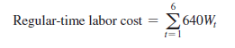
• Regular-time labor cost. Recall that workers are paid a regular-time wage of $640 ($4/hour X 8 hours/day X 20 days/month) per month. Because W t is the number of workers in Period t, the regular-time labor cost over the planning horizon is given by

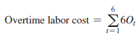
• Overtime labor cost. As overtime labor cost is $6 per hour (see Table 8-3) and O t represents the number of overtime hours worked in Period t, the overtime cost over the planning horizon is

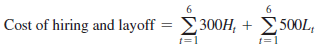
• Cost of hiring and layoffs. The cost of hiring a worker is $300 and the cost of laying off a worker is $500 (see Table 8-3). H t and L t represent the number hired and the number laid off, respectively, in Period Thus, the cost of hiring and layoff is given by

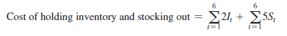
• Cost of inventory and stockout. The cost of carrying inventory is $2 per unit per month, and the cost of stocking out is $5 per unit per month (see Table 8-3). I t and S t represent the units in inventory and the units stocked out, respectively, in Period Thus, the cost of holding inventory and stocking out is

• Cost of materials and subcontracting. The material cost is $10 per unit and the sub­contracting cost is $30/unit (see Table 8-3). P t represents the quantity produced and C t represents the quantity subcontracted in Period t. Thus, the material and subcontracting cost is

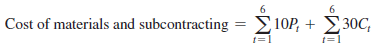
The total cost incurred during the planning horizon is the sum of all the aforementioned costs and is given by

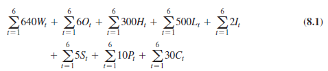
Red Tomato’s objective is to find an aggregate plan that minimizes the total cost (Equation 8.1) incurred during the planning horizon.

The values of the decision variables in the objective function cannot be set arbitrarily. They are subject to a variety of constraints defined by available capacity and operating policies. The next step in setting up the aggregate planning model is to define clearly the constraints linking the decision variables.

3. Constraints

Red Tomato’s vice president must now specify the constraints that the decision variables must not violate. They are as follows:

• Workforce, hiring, and layoff constraints . The workforce size W t in Period t is obtained by adding the number hired H t in Period t to the workforce size W t- 1 in Period t – 1, and subtracting the number laid off L t in Period t as follows:

Wt = Wt – 1 + Ht – Lt   for    t = 1, . . . , 6                    ( 8.2)

• Capacity constraints . In each period, the amount produced cannot exceed the avail­able capacity. This set of constraints limits the total production by the total internally available capacity (which is determined based on the available labor hours, regular or overtime). Subcon­tracted production is not included in this constraint because the constraint is limited to produc­tion within the plant. As each worker can produce 40 units per month on regular time (four hours per unit as specified in Table 8-3) and one unit for every four hours of overtime, we have the following:

• Inventory balance constraints . The third set of constraints balances inventory at the end of each period. Net demand for Period t is obtained as the sum of the current demand D t and the previous backlog S t -1 . This demand is either filled from current production (in-house production P t or subcontracted production C t ) and previous inventory I t _ 1 (in which case some inventory I t may be left over) or part of it is backlogged S t . This relationship is captured by the following equation:

It _ 1 + Pt + Ct = Dt + St _ i + It _ St for t = 1, . . . , 6                                        (8.4)

The starting inventory is given by I 0 = 1,000, the ending inventory must be at least 500 units (i.e., I 6 > 500), and initially there are no backlogs (i.e., S 0 = 0).

• Overtime limit constraints . The fourth set of constraints requires that no employee work more than 10 hours of overtime each month. This requirement limits the total amount of overtime hours available as follows:

O t < 10W t for t = 1, . . . , 6                                                            (8.5)

In addition, each variable must be nonnegative and there must be no backlog at the end of Period 6 (i.e., S 6 = 0).

When implementing the model in Microsoft Excel, which we discuss later, it is easiest if all the constraints are written so the right-hand side for each constraint is 0. The overtime limit constraint (Equation 8.5) in this form is written as

O t _ 10W t < 0 for t = 1, . . . , 6

Observe that one can easily add constraints that limit the amount purchased from subcontrac­tors each month or the maximum number of employees to be hired or laid off. Any other con­straints limiting backlogs or inventories can also be accommodated. Ideally, the number of employees hired or laid off should be integer variables. Fractional variables may be justified if some employees work for only part of a month. Such a linear program can be solved using the tool Solver in Excel.

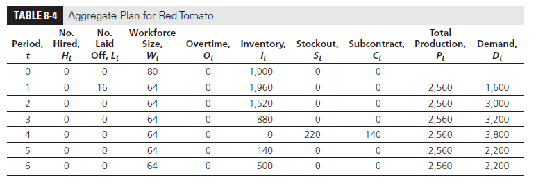
By optimizing the objective function (minimizing cost in Equation 8.1) subject to the listed constraints (Equations 8.2 to 8.5), the vice president obtains the aggregate plan shown in Table 8-4. (Later in the chapter, we discuss how to perform this optimization using Excel with the spread­sheet Chapter8,9-examples.)

For this aggregate plan, we have the following:

Total cost over planning horizon = $422,660

Red Tomato lays off a total of 16 employees at the beginning of January. After that, the company maintains the workforce and production level. It uses the subcontractor during the month of April. Red Tomato carries a backlog only from April to May; in all other months, it plans no stockouts. In fact, it carries inventory in all other periods. We describe this inventory as seasonal inventory because it is carried in anticipation of a future increase in demand.

If the seasonal fluctuation of demand grows, synchronization of supply and demand becomes more difficult, resulting in an increase in either inventory or backlogs as well as an increase in the total cost to the supply chain. This is illustrated in Example 8-1, in which the demand forecast is more variable.

EXAMPLE 8-1 Impact of Higher Demand Variability

All the data are exactly the same as in our previous discussion of Red Tomato, except for the demand forecast. Assume that the same overall demand (16,000 units) is distributed over the six months in such a way that the seasonal fluctuation of demand is higher, as shown in Table 8-5. Obtain the optimal aggregate plan in this case.

In this case, the optimal aggregate plan (using the same costs as those used before) is shown in Table 8-6.

Observe that monthly production remains the same, but both inventories and stockouts (backlogs) go up compared to the aggregate plan in Table 8-4 for the demand profile in Table 8-2. The cost of meeting the new demand profile in Table 8-5 is higher, at $433,080 (compared to $422,660 for the previous demand profile in Table 8-2).

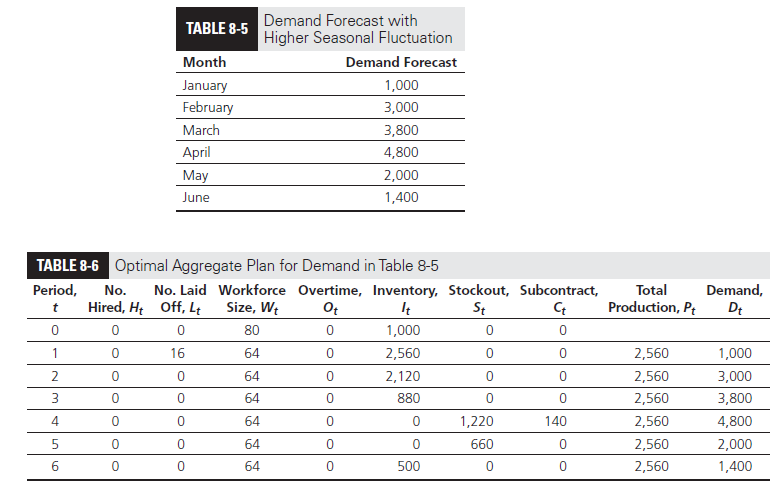
From Example 8-1, we can see that the increase in demand variability at the retailer increases seasonal inventory as well as planned costs.

Using the Red Tomato example, we also see that the optimal trade-off changes as the costs change. This is illustrated in Example 8-2, in which we show that as the costs of hiring and layoff decrease, it is better to vary capacity with demand while having less inventory and fewer backlogs.

EXAMPLE 8-2 Impact of Lower Costs of Hiring and Layoff

Assume that demand at Red Tomato is as shown in Table 8-2, and all other data are the same except that the costs of hiring and layoff are now $50 each. Evaluate the total cost corresponding to the aggregate plan in Table 8-4. Suggest an optimal aggregate plan for the new cost structure.

If the costs of hiring and layoff decrease to $50 each, the cost corresponding to the aggregate plan in Table 8-4 decreases from $422,660 to $412,770. Taking this new cost into account and determining a new optimal aggregate plan yields the plan shown in Table 8-7. Observe that the workforce size fluctuates between a high of 88 and a low of 45, as opposed to being stable at 64 as in Table 8-4.

As expected, the workforce size is varied (because the cost of varying capacity has decreased), whereas inventory and stockouts have decreased compared with the aggregate plan in Table 8-4. The total cost of the aggregate plan in Table 8-7 is $412,770, compared with $422,660 (for the aggregate plan in Table 8-4) if the costs of hiring and layoff are $50 each.

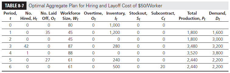
From Example 8-2, observe that increasing volume flexibility (by decreasing the cost of hiring and layoff) not only decreases the total cost but also shifts the optimal balance toward using the volume flexibility while carrying lower inventories and allowing less stockout.

In the next section, we explain how to implement the linear programming methodology for aggregate planning using Microsoft Excel.

Source: Chopra Sunil, Meindl Peter (2014), Supply Chain Management: Strategy, Planning, and Operation , Pearson; 6th edition.

14 Jun 2021

15 Jun 2021

4 thoughts on “ Aggregate Planning Using Linear Programming in a Supply Chain ”

I’m curious to find out what blog system you have been utilizing? I’m having some small security issues with my latest site and I would like to find something more safeguarded. Do you have any solutions?

Nice post. I learn something totally new and challenging on websites I stumbleupon on a daily basis. It’s always exciting to read through articles from other authors and use a little something from their web sites.

Great article! We will be linking to this great article on our site.

Keep up the good writing.

Nice post. I learn something new and challenging on blogs I stumbleupon every day. It’s always interesting to read through content from other writers and use a little something from their sites.

Leave a Reply Cancel reply

Your email address will not be published. Required fields are marked *

Save my name, email, and website in this browser for the next time I comment.

Username or email address  *

Password  *

Log in Remember me

Lost your password?

Navigation Menu

Search code, repositories, users, issues, pull requests..., provide feedback.

We read every piece of feedback, and take your input very seriously.

Saved searches

Use saved searches to filter your results more quickly.

To see all available qualifiers, see our documentation .

• Notifications You must be signed in to change notification settings

Red Tomato Gardening Tools and Sporting Goods Company. Demand forecast optimization problem model using Python, Pyomo and GLPK in Python. Multifactor objectives and constraints solved using algebraic formulation to allocate and minimize cost. Excel Solver used to allocate how much of each product to produce so that profit is maximized

bryce-bowles/Red-Tomato-gardening-tools

Folders and files.

Repository files navigation

Red-tomato-gardening-tools.

Red Tomato Gardening Tools

March 09, 2020

• (from Chopra and Meindl, Ch. 8). Solve using Pyomo. The demand for Red Tomato Tools gardening tools is highly seasonal, peaking in the summer when people plant their gardens. Red Tomato has decided to use aggregate planning to overcome this obstacle of seasonal demand and maximize their profits. The options Red Tomato has for handling the seasonality are adding workers during the peak season, subcontracting out some of the work, building up inventory during the slow months and building up backlog of orders that will be delivered late to customers.

To determine how to best use these options through an aggregate plan, Red Tomato’s VP for Supply Chain Operations starts with demand forecasts for its tools over the next six months. These are shown in Table 1.

Red Tomato sells each tool to retailers for $40. The company has a starting inventory in January of 1,000 tools. At the beginning of January, the company has a work-force of 80 employees. The plant has a total of 20 working days each month, and each employee earns $4.00 per hour regular time. Each employee works a total of eight hours a day on straight time and the rest on overtime. The capacity of the production operation is determined primarily by the total labor hours worked. Due to labor rules, no employee works more than 10 hours of overtime per month.

Other costs are shown in Table 2. Currently, Red Tomato has no limits on subcontracting, inventories and stock-outs/backlogs. All stock-outs are backlogged and supplied from the following month’s production. Inventory costs are incurred on the ending inventory in the month. The supply chain planner’s goal is to obtain the optimal aggregate plan that allows Red Tomato to end June with at least 500 units which means no stock-outs at the end of June and at least 500 units of inventory.

The optimal aggregate plan is one that results in the highest profit over the six-month planning horizon. Given Red Tomato’s desire for a very high level of customer service, we will assume all demand is met. Therefore, revenues earned over the planning horizon are fixed given the fixed price. In this case, minimizing cost over the planning horizon is the same as maximizing profit.

Table 2: Costs for Red Tomato

3 Objective in Words Decide how much to produce each month so that total cost is minimized (profit is maximized) while demand is met. Minimizing cost of: * Cost of regular time labor * Cost of overtime labor * Cost of hiring * Cost of layoffs * Cost of holding inventory * Cost of stocking out * Cost of subcontracting * Cost of materials

Subject to: * Demand being met * Due to labor rules, no employee works more than 10 hours of overtime per month * No Stockouts at the end of June * End June with at least 500 units of inventory

4 Algebraic Formulation Decision Variables:

5 Implementation See attached file, HW_3_RedTomatoes.ipynb and RedTomatoes.xlsx, for the implementation and solution of the model using Pyomo and GLPK in Python.

6 Results and Interpretation The optimal solution for Red Tomatoes is…   Sporting Goods Company Problem Solution

1 Problem (from Taylor 3.7). A sporting goods company makes basketballs and footballs. Each product is produced from two resources - rubber and leather. Each basketball produced results in a profit of $12 and each football earns $16 in profit. The resource requirements for each product are: basketball (3 lb rubber, 4 sq ft leather) and football (2 lb rubber and 5 sq ft leather). There are 500 lb of rubber and 800 sq ft of leather available. For your implementation, implement and solve the problem using Microsoft Excel and turn in your workbook. In addition, answer the following questions, explaining your reasoning: How much does the profit need to change per basketball before it is optimal to produce basketballs? Suppose a source for leather offers 100 square feet at $3 per square foot. Should the company make the purchase? Suppose a source for rubber offers 100 pounds at $3 per pound. Should the company make the purchase? What would be the effect on the optimal solution if the profit for a basketball changed from $12 to $13? What would be the effect on the optimal solution if the profit for a football changed from $16 to $15.50? Update 2/27: For both problems, you do not need to specify that the decision variables are integer. Assume that fractional values are acceptable.

Let 1. P = {Basketball, Football} be the set of products 2. profit〗_i = profit ($) for product i, i∈P; 3. rubberAval = rubber available for either product 4. leatherAval = leather available for either product   3 Objective\ in Words: Decide how much of each product to produce so that profit is maximized * At most, 500 lb’s of rubber are used * At most, 800 sq ft are used

4 Algebraic Formulation

5 Implementation See attached file, HW3sporting_goods.xlsx, for the implementation and solution of the model using Excel Solver.

6 Interpret the Results

• Jupyter Notebook 100.0%