average case analysis for insertion sort

Reset password New user? Sign up

Existing user? Log in

Insertion Sort

Already have an account? Log in here.

Insertion sort is a sorting algorithm that builds a final sorted array (sometimes called a list) one element at a time. While sorting is a simple concept, it is a basic principle used in complex computer programs such as file search, data compression, and path finding. Running time is an important thing to consider when selecting a sorting algorithm since efficiency is often thought of in terms of speed. Insertion sort has an average and worst-case running time of \(O(n^2)\), so in most cases, a faster algorithm is more desirable.

The Sorting Problem

Insertion sort implementation, complexity of insertion sort.

An algorithm that maps the following input/output pair is called a sorting algorithm : Input: An array \(A\) that contains \(n\) orderable elements \(A[0,1,...,n-1]\). Output: A sorted permutation of \(A\), called \(B\), such that \(B[0] \leq B[1] \leq \cdots \leq B[n-1].\) \(_\square\)

Here is what it means for an array to be sorted .

An array \(<a_n>\) is sorted if and only if for all \(i<j\), \(a_i \leq a_j.\)

In other words, a sorted array is an array that is in a particular order. For example, \([a,b,c,d]\) is sorted alphabetically, \([1,2,3,4,5]\) is a list of integers sorted in increasing order, and \([5,4,3,2,1]\) is a list of integers sorted in decreasing order.

By convention, empty arrays and singleton arrays (arrays consisting of only one element) are always sorted. This is a key point for the base case of many sorting algorithms.

The insertion sort algorithm iterates through an input array and removes one element per iteration, finds the place the element belongs in the array, and then places it there. This process grows a sorted list from left to right. The algorithm is as follows:

For each element \(A[i]\), if \(A[i]\) \(\gt \) \(A[i+1]\), swap the elements until \(A[i]\) \(\leq \) \(A[i+1]\).

The animation below illustrates insertion sort:

Sort the following array using insertion sort. \(A = [8,2,4,9,3,6]\) [1]

Another way to visualize insertion sort is to think of a stack of playing cards.

You have the cards 3, 9, 6, 5, and 7. Write an algorithm or pseudo-code that arranges the values of the cards in ascending order. Basically, the idea is to run insertion sort \(n -1\) times and find the index at which each element should be inserted. Here is some pseudocode. [2] 1 2 3 4 5 6 7 8 9 for i = 1 to length(A) x = A[i] j = i - 1 while j >= 0 and A[j] > x A[j+1] = A[j] j = j - 1 end while A[j+1] = x end for The sorted array is [3, 5, 6, 7, 9]. \(_\square\)

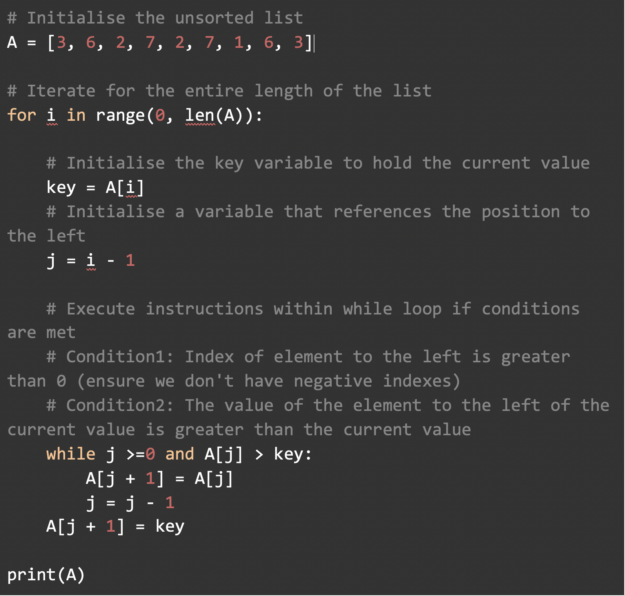
Here is one way to implement insertion sort in Python. There are other ways to implement the algorithm, but all implementations stem from the same ideas. Insertion sort can sort any orderable list. 1 2 3 4 5 6 7 8 9 def insertion_sort ( array ): for slot in range ( 1 , len ( array )): value = array [ slot ] test_slot = slot - 1 while test_slot > - 1 and array [ test_slot ] > value : array [ test_slot + 1 ] = array [ test_slot ] test_slot = test_slot - 1 array [ test_slot + 1 ] = value return array

The above Python code sorts a list in increasing order. What single change could you make to have insertion sort sort in decreasing order? Show Answer Flip the second greater than sign to a less than sign in line 5. Line 5 should read: while test slot > -1 and array[test slot] < value: #flip this sign

Insertion sort runs in \(O(n)\) time in its best case and runs in \(O(n^2)\) in its worst and average cases.

Best Case Analysis: Insertion sort performs two operations: it scans through the list, comparing each pair of elements, and it swaps elements if they are out of order. Each operation contributes to the running time of the algorithm. If the input array is already in sorted order, insertion sort compares \(O(n)\) elements and performs no swaps (in the Python code above, the inner loop is never triggered). Therefore, in the best case, insertion sort runs in \(O(n)\) time.

Worst and Average Case Analysis: The worst case for insertion sort will occur when the input list is in decreasing order. To insert the last element, we need at most \(n-1\) comparisons and at most \(n-1\) swaps. To insert the second to last element, we need at most \(n-2\) comparisons and at most \(n-2\) swaps, and so on. [3] The number of operations needed to perform insertion sort is therefore: \(2 \times (1+2+ \dots +n-2+n-1)\). To calculate the recurrence relation for this algorithm, use the following summation: \[ \sum_{q=1}^{p} q = \frac{p(p+1)}{2}. \] It follows that \[ \frac{2(n-1)(n-1+1)}{2}=n(n-1). \] Use the master theorem to solve this recurrence for the running time. As expected, the algorithm's complexity is \( O(n^2).\) When analyzing algorithms, the average case often has the same complexity as the worst case. So insertion sort, on average, takes \( O(n^2)\) time.

Insertion sort has a fast best-case running time and is a good sorting algorithm to use if the input list is already mostly sorted. For larger or more unordered lists, an algorithm with a faster worst and average-case running time, such as mergesort , would be a better choice.

Insertion sort is a stable sort with a space complexity of \(O(1)\).

For the following list, which two sorting algorithms have the same running time (ignoring constant factors)?

\[A = [4,2,0,9,8,1]\]

• Devadas , S. 6.006 Introduction to Algorithms: Lecture 3, Fall 2011 . Retrieved March, 24, 2016, from http://ocw.mit.edu/courses/electrical-engineering-and-computer-science/6-006-introduction-to-algorithms-fall-2011/lecture-videos/MIT6_006F11_lec03.pdf
• Cormen, T., Leiserson, C., Rivest, R., & Stein, C. (2001). Introduction to Algorithms (2nd edition) (pp. 15-21). The MIT Press.
• Sinapova , L. Sorting Algorithms: Insertion Sort . Retrieved March, 24, 2016, from http://faculty.simpson.edu/lydia.sinapova/www/cmsc250/LN250_Weiss/L11-InsSort.htm

Problem Loading...

Note Loading...

Set Loading...

Search anything:

Time Complexity of Insertion Sort

Algorithms sorting algorithms time complexity.

Open-Source Internship opportunity by OpenGenus for programmers. Apply now.

Reading time: 15 minutes | Coding time: 5 minutes

In this article, we have explored the time and space complexity of Insertion Sort along with two optimizations. Before going into the complexity analysis, we will go through the basic knowledge of Insertion Sort. In short:

• The worst case time complexity of Insertion sort is O(N^2)
• The average case time complexity of Insertion sort is O(N^2)
• The time complexity of the best case is O(N) .
• The space complexity is O(1)

What is Insertion Sort?

Insertion sort is one of the intutive sorting algorithm for the beginners which shares analogy with the way we sort cards in our hand. As the name suggests, it is based on "insertion" but how? An array is divided into two sub arrays namely sorted and unsorted subarray. How come there is a sorted subarray if our input in unsorted?

The algorithm is based on one assumption that a single element is always sorted.

Hence, the first element of array forms the sorted subarray while the rest create the unsorted subarray from which we choose an element one by one and "insert" the same in the sorted subarray. The same procedure is followed until we reach the end of the array.

In each iteration, we extend the sorted subarray while shrinking the unsorted subarray.

Working Principle

• Compare the element with its adjacent element.
• If at every comparison, we could find a position in sorted array where the element can be inserted, then create space by shifting the elements to right and insert the element at the appropriate position .
• Repeat the above steps until you place the last element of unsorted array to its correct position.

Let's take an example. Input: 15, 9, 30, 10, 1 Expected Output: 1, 9, 10, 15, 30 The steps could be visualized as:

• Worst case time complexity: Θ(n^2)
• Average case time complexity: Θ(n^2)
• Best case time complexity: Θ(n)
• Space complexity: Θ(1)

Implementation

Complexity analysis for insertion sort.

We examine Algorithms broadly on two prime factors, i.e.,

Running Time

Running Time of an algorithm is execution time of each line of algorithm

As stated, Running Time for any algorithm depends on the number of operations executed. We could see in the Pseudocode that there are precisely 7 operations under this algorithm. So, our task is to find the Cost or Time Complexity of each and trivially sum of these will be the Total Time Complexity of our Algorithm. We assume Cost of each i operation as C i where i ∈ {1,2,3,4,5,6,8} and compute the number of times these are executed. Therefore the Total Cost for one such operation would be the product of Cost of one operation and the number of times it is executed. We could list them as below:

Then Total Running Time of Insertion sort (T(n)) = C 1 * n + ( C 2 + C 3 ) * ( n - 1 ) + C 4 * Σ n - 1 j = 1 ( t j ) + ( C 5 + C 6 ) * Σ n - 1 j = 1 ( t j ) + C 8 * ( n - 1 )

Memory usage

Memory required to execute the Algorithm.

As we could note throughout the article, we didn't require any extra space. We are only re-arranging the input array to achieve the desired output. Hence, we can claim that there is no need of any auxiliary memory to run this Algorithm. Although each of these operation will be added to the stack but not simultaneoulsy the Memory Complexity comes out to be O(1)

Best Case Analysis

In Best Case i.e., when the array is already sorted, t j = 1 Therefore,T( n ) = C 1 * n + ( C 2 + C 3 ) * ( n - 1 ) + C 4 * ( n - 1 ) + ( C 5 + C 6 ) * ( n - 2 ) + C 8 * ( n - 1 ) which when further simplified has dominating factor of n and gives T(n) = C * ( n ) or O(n)

Worst Case Analysis

In Worst Case i.e., when the array is reversly sorted (in descending order), t j = j Therefore,T( n ) = C 1 * n + ( C 2 + C 3 ) * ( n - 1 ) + C 4 * ( n - 1 ) ( n ) / 2 + ( C 5 + C 6 ) * ( ( n - 1 ) (n ) / 2 - 1) + C 8 * ( n - 1 ) which when further simplified has dominating factor of n 2 and gives T(n) = C * ( n 2 ) or O( n 2 )

Average Case Analysis

Let's assume that t j = (j-1)/2 to calculate the average case Therefore,T( n ) = C 1 * n + ( C 2 + C 3 ) * ( n - 1 ) + C 4 /2 * ( n - 1 ) ( n ) / 2 + ( C 5 + C 6 )/2 * ( ( n - 1 ) (n ) / 2 - 1) + C 8 * ( n - 1 ) which when further simplified has dominating factor of n 2 and gives T(n) = C * ( n 2 ) or O( n 2 )

Can we optimize it further?

Searching for the correct position of an element and Swapping are two main operations included in the Algorithm.

We can optimize the searching by using Binary Search , which will improve the searching complexity from O(n) to O(log n) for one element and to n * O(log n) or O(n log n) for n elements. But since it will take O(n) for one element to be placed at its correct position, n elements will take n * O(n) or O(n 2 ) time for being placed at their right places. Hence, the overall complexity remains O(n 2 ) .

We can optimize the swapping by using Doubly Linked list instead of array, that will improve the complexity of swapping from O(n) to O(1) as we can insert an element in a linked list by changing pointers (without shifting the rest of elements). But since the complexity to search remains O(n 2 ) as we cannot use binary search in linked list. Hence, The overall complexity remains O(n 2 ) .

Therefore, we can conclude that we cannot reduce the worst case time complexity of insertion sort from O(n 2 ) .

• Simple and easy to understand implementation
• Efficient for small data
• If the input list is sorted beforehand (partially) then insertions sort takes O(n+d) where d is the number of inversions
• Chosen over bubble sort and selection sort, although all have worst case time complexity as O(n^2)
• Maintains relative order of the input data in case of two equal values (stable)
• It requires only a constant amount O(1) of additional memory space (in-place Algorithm)

Applications

• It could be used in sorting small lists .
• It could be used in sorting "almost sorted" lists .
• It could be used to sort smaller sub problem in Quick Sort .

DEV Community

Posted on Mar 19, 2020 • Updated on May 2, 2020

Insertion Sort: Algorithm Analysis

Hola, first things first, thanks for making it to this article. The last one was a tough one, no? Just for me? Okay then (^__^)!

We analyze space and time complexity of an algorithm to see how efficient it is and whether we should go with it or design a new one according to our needs (the amount of data, the operations we need to perform and so on).

There are three kinds of analysis namely the worst case, best case, and average case.

There are five asymptotic notations -

• Big-Oh: upper bound of an algorithm
• Big-Omega: lower bound of an algorithm
• Theta: lower and upper bound (tight bound) of an algorithm
• Little-oh: upper bound that is not asymptotically tight
• Little-omega: lower bound that is not asymptotically tight

Insertion Sort

Sorting is a very common problem in Computer Science and is asked often in coding interviews and tests. As the name suggests, sorting basically means converting an unsorted input like [1,10,5,8,2] to a sorted output like [1,2,5,8,10], increasing order unless specified otherwise.

Insertion sort is a common way of sorting and is illustrated below -

Credits - GeeksForGeeks You probably know this but GfG is one of the best sources for learning many topics in Computer Science. So, if you ever feel stuck or if you have a doubt, go read the GfG article for that topic.

Now, let's go through the pseudocode for Insertion Sort but you may ask what is Pseudocode? Here you go.

Pseudocode -

It is an informal way of writing programs that do not require any strict programming language syntax. We describe algorithms in Pseudocode so that people who know any programming language can understand it easily. One important point to note is that in pseudocode, index (of arrays, etc.) generally starts from 1 as opposed to 0 in programming languages. The pseudocode for Insertion Sort is -

That's it. Simple, eh? If you have any doubts, I would be happy to elaborate in the comments section.

Now, let's analyze the performance of insertion sort, using the concepts we learned in the previous article.

The cost for i th step is c i . The cost for any comment is 0 since it's not performed and is just for the programmer's understanding. Hence, insertion sort is essentially a seven-step algorithm.

Now, steps 1, 2, 4 and 8 will run n-1 times (from second to the last element).

Step 5 will run t j times (assumption) for n-1 elements (second till last). Similarly, steps 6 and 7 will run t j -1 times for n-1 elements. They will run one less time because for each element - before line 8 is executed, while condition (step 5) is checked/executed but steps 6 and 7 ain't as the condition in while statement fails.

Now we analyze the best, worst and average case for Insertion Sort.

Best case -

The array is already sorted. t j will be 1 for each element as while condition will be checked once and fail because A[i] is not greater than key .

We can express this running time as an+b where a and b are constants that depend on costs c i . Hence, running time is a linear function of size n , that is, the number of elements in the array.

Worst case -

The array is reverse sorted. t j will be j for each element as key will be compared with each element in the sorted array and hence, while condition will be checked j-1 times for comparing key with all elements in the sorted array plus one more time when i becomes 0 (after which i > 0 will fail, control goes to step 8).

The explanation for the first summation is simple - the sum of numbers from 1 to n is n(n+1)/2, since the summation starts from 2 and not 1, we subtract 1 from the result. We can simplify the second summation similarly by replacing n by n-1 in the first summation.

Average case -

The average case running time is the same as the worst-case (a quadratic function of n). On average, half the elements in A[1..j-1]􏰂 are less than A[j] 􏰂, and half the elements are greater. On average, therefore, we check half of the subarray A[1..j-1], and so t j is about j/2. The resulting average-case running time turns out to be a quadratic function of the input size, just like the worst-case running time.

That's it for today. If you have any reviews/suggestions, please tell them in the comments section. In the next article, we will go through various techniques for finding

Top comments (0)

Templates let you quickly answer FAQs or store snippets for re-use.

Are you sure you want to hide this comment? It will become hidden in your post, but will still be visible via the comment's permalink .

Hide child comments as well

For further actions, you may consider blocking this person and/or reporting abuse

3075. Maximize Happiness of Selected Children

MD ARIFUL HAQUE - May 9

Find First and Last Position of Element in Sorted Array | LeetCode | Java

Alysa - May 16

Computer Vision Meetup: Making LLMs Safe & Reliable

Jimmy Guerrero - May 2

Difference between Data Analysts, Data Scientists, and Data Engineers

Onumaku Chibuike Victory - May 6

We're a place where coders share, stay up-to-date and grow their careers.

Insertion Sort - Algorithm, Source Code, Time Complexity

Article Series: Sorting Algorithms

Part 1: Introduction

Part 2: Sorting in Java

Part 3: Insertion Sort

Part 4: Selection Sort

Part 5: Bubble Sort

Part 6: Quicksort

Part 7: Merge Sort

Part 8: Heapsort

Part 9: Counting Sort

Part 10: Radix Sort

(Sign up for the HappyCoders Newsletter to be immediately informed about new parts.)

This article is part of the series " Sorting Algorithms: Ultimate Guide " and…

• describes how Insertion Sort works,
• shows an implementation in Java,
• explains how to derive the time complexity,
• and checks whether the performance of the Java implementation matches the expected runtime behavior.

You can find the source code for the entire article series in my GitHub repository .

Example: Sorting Playing Cards

Let us start with a playing card example.

Imagine being handed one card at a time. You take the first card in your hand. Then you sort the second card to the left or right of it. The third card is placed to the left, in between or to the right, depending on its size. And also, all the following cards are placed in the right position.

Have you ever sorted cards this way before?

If so, then you have intuitively used "Insertion Sort".

Insertion Sort Algorithm

Let's move from the card example to the computer algorithm. Let us assume we have an array with the elements [6, 2, 4, 9, 3, 7]. This array should be sorted with Insertion Sort in ascending order.

First, we divide the array into a left, sorted part, and a right, unsorted part. The sorted part already contains the first element at the beginning, because an array with a single element can always be considered sorted.

Then we look at the first element of the unsorted area and check where, in the sorted area, it needs to be inserted by comparing it with its left neighbor.

In the example, the 2 is smaller than the 6, so it belongs to its left. In order to make room, we move the 6 one position to the right and then place the 2 on the empty field. Then we move the border between sorted and unsorted area one step to the right:

We look again at the first element of the unsorted area, the 4. It is smaller than the 6, but not smaller than the 2 and, therefore, belongs between the 2 and the 6. So we move the 6 again one position to the right and place the 4 on the vacant field:

The next element to be sorted is the 9, which is larger than its left neighbor 6, and thus larger than all elements in the sorted area. Therefore, it is already in the correct position, so we do not need to shift any element in this step:

The next element is the 3, which is smaller than the 9, the 6 and the 4, but greater than the 2. So we move the 9, 6 and 4 one position to the right and then put the 3 where the 4 was before:

That leaves the 7 – it is smaller than the 9, but larger than the 6, so we move the 9 one field to the right and place the 7 on the vacant position:

The array is now completely sorted.

Insertion Sort Java Source Code

The following Java source code shows how easy it is to implement Insertion Sort.

The outer loop iterates – starting with the second element, since the first element is already sorted – over the elements to be sorted. The loop variable i, therefore, always points to the first element of the right, unsorted part.

In the inner while loop, the search for the insert position and the shifting of the elements is combined:

• searching in the loop condition: until the element to the left of the search position j is smaller than the element to be sorted,
• and shifting the sorted elements in the loop body.

The code shown differs from the code in the GitHub repository in two ways: First, the InsertionSort class in the repository implements the SortAlgorithm interface to be easily interchangeable within my test framework.

On the other hand, it allows the specification of start and end index, so that sub-arrays can also be sorted. This will later allow us to optimize Quicksort by having sub-arrays that are smaller than a certain size sorted with Insertion Sort instead of dividing them further.

Insertion Sort Time Complexity

We denote with n the number of elements to be sorted; in the example above n = 6 .

The two nested loops are an indication that we are dealing with quadratic effort, meaning with time complexity of O(n²) *. This is the case if both the outer and the inner loop count up to a value that increases linearly with the number of elements.

With the outer loop, this is obvious as it counts up to n .

And the inner loop? We'll analyze that in the next three sections.

* In this article , I explain the terms "time complexity" and "Big O notation" using examples and diagrams.

Average Time Complexity

Let's look again at the example from above where we have sorted the array [6, 2, 4, 9, 3, 7].

In the first step of the example, we defined the first element as already sorted; in the source code, it is simply skipped.

In the second step, we shifted one element from the sorted array. If the element to be sorted had already been in the right place, we would not have had to shift anything. This means that we have an average of 0.5 move operations in the second step.

In the third step, we have also shifted one element. But here it could also have been zero or two shifts. On average, it is one shift in this step.

In step four, we did not need to shift any elements. However, it could have been necessary to shift one , two , or three elements; the average here is 1.5.

In step five, we have on average two shift operations:

And in step six, 2.5:

So in total we have on average 0.5 + 1 + 1.5 + 2 + 2.5 = 7.5 shift operations.

We can also calculate this as follows:

Six elements times five shifting operations; divided by two, because on average over all steps, half of the cards are already sorted; and again divided by two, because on average, the element to be sorted has to be moved to the middle of the already sorted elements:

6 × 5 × ½ × ½   =   30 × ¼   =   7,5

The following illustration shows all steps once again:

If we replace 6 with n , we get

n × (n - 1) × ¼

When multiplied, that's:

The highest power of n in this term is n² ; the time complexity for shifting is, therefore, O(n²) . This is also called "quadratic time".

So far, we have only looked at how the sorted elements are shifted – but what about comparing the elements and placing the element to be sorted on the field that became free?

For comparison operations, we have one more than shift operations (or the same amount if you move an element to the far left). The time complexity for the comparison operations is, therefore, also O(n²) .

The element to be sorted must be placed in the correct position as often as there are elements minus those that are already in the right position – so n-1 times at maximum. Since there is no n² here, but only an n , we speak of "linear time", noted as O(n) .

When considering the overall complexity, only the highest level of complexity counts (see " Big O Notation and Time Complexity – Easily Explained "). Therefore follows:

The average time complexity of Insertion Sort is: O(n²)

Where there is an average case , there is also a worst and a best case .

Worst-Case Time Complexity

In the worst case, the elements are sorted completely descending at the beginning. In each step, all elements of the sorted sub-array must, therefore, be shifted to the right so that the element to be sorted – which is smaller than all elements already sorted in each step – can be placed at the very beginning.

In the following diagram, this is demonstrated by the fact that the arrows always point to the far left:

The term from the average case , therefore, changes in that the second dividing by two is omitted:

n × (n - 1) × ½

When we multiply this out, we get:

Even if we have only half as many operations as in the average case, nothing changes in terms of time complexity – the term still contains n² , and therefore follows:

The worst-case time complexity of Insertion Sort is: O(n²)

Best-Case Time Complexity

The best case becomes interesting!

If the elements already appear in sorted order, there is precisely  one comparison in the inner loop and no swap operation at all.

With n elements, that is, n-1 steps (since we start with the second element), we thus come to n-1 comparison operations. Therefore:

The best-case time complexity of Insertion Sort is: O(n)

Insertion Sort With Binary Search?

Couldn't we speed up the algorithm by searching the insertion point with binary search ? This is much faster than the sequential search – it has a time complexity of O(log n) .

Yes, we could. However, we would not have gained anything from this, because we would still have to shift each element from the insertion position one position to the right, which is only possible step by step in an array. Thus the inner loop would remain at linear complexity despite the binary search. And the whole algorithm would remain at quadratic complexity, that is O(n²) .

Insertion Sort With a Linked List?

If the elements are in a linked list, couldn't we insert an element in constant time, O(1) ?

Yeah, we could. However, a linked list does not allow for a binary search. This means that we would still have to iterate through all sorted elements in the inner loop to find the insertion position. This, in turn, would result in linear complexity for the inner loop and quadratic complexity for the entire algorithm.

Runtime of the Java Insertion Sort Example

After all this theory, it's time to check it against the Java implementation presented above.

The UltimateTest class from the GitHub repository executes Insertion Sort (and all other sorting algorithms presented in this series of articles) as follows:

• for different array sizes, starting at 1,024, then doubled in each iteration up to 536,870,912 (trying to create an array with 1,073,741,824 elements leads to a "Native memory allocation" error) – or until a test takes more than 20 seconds;
• with unsorted, ascending and descending sorted elements;
• with two warm-up rounds to allow the HotSpot compiler to optimize the code;
• then repeated until the program is aborted.

After each iteration, the test program prints out the median of the previous measurement results.

Here is the result for Insertion Sort after 50 iterations (this is only an excerpt for the sake of clarity; the complete result can be found here ):

It is easy to see

• how the runtime roughly quadruples when doubling the amount of input for unsorted and descending sorted elements,
• how the runtime in the worst case is twice as long as in the average case,
• how the runtime for pre-sorted elements grows linearly and is significantly smaller.

This corresponds to the expected time complexities of O(n²) and O(n) .

Here the measured values as a diagram:

With pre-sorted elements, Insertion Sort is so fast that the line is hardly visible. Therefore here is the best case separately:

Other Characteristics of Insertion Sort

The space complexity of Insertion Sort is constant since we do not need any additional memory except for the loop variables i and j and the auxiliary variable elementToSort. This means that – no matter whether we sort ten elements or a million – we always need only these three additional variables. Constant complexity is noted as O(1) .

The sorting method is stable because we only move elements that are greater than the element to be sorted (not "greater or equal"), which means that the relative position of two identical elements never changes.

Insertion Sort is not directly parallelizable.* However, there is a parallel variant of Insertion Sort: Shellsort ( here its description on Wikipedia ).

* You could search binary and then parallelize the shifting of the sorted elements. But this would only make sense with large arrays, which would have to be split exactly along the cache lines in order not to lose the performance gained by parallelization – or to even reverse it into the opposite direction – due to synchronization effects. This effort can be saved since there are more efficient sorting algorithms for larger arrays anyway.

Insertion Sort vs. Selection Sort

You can find a comparison of Insertion Sort and Selection Sort in the article about Selection Sort .

Insertion Sort is an easy-to-implement, stable sorting algorithm with time complexity of O(n²) in the average and worst case , and O(n) in the best case .

For very small n , Insertion Sort is faster than more efficient algorithms such as Quicksort or Merge Sort. Thus these algorithms solve smaller sub-problems with Insertion Sort (the Dual-Pivot Quicksort implementation in Arrays.sort() of the JDK, for example, for less than 44 elements).

You will find more sorting algorithms in this overview of all sorting algorithms and their characteristics in the first part of the article series.

If you liked the article, feel free to share it using one of the share buttons at the end. Would you like to be informed by e-mail when I publish a new article? Then click here to subscribe to the HappyCoders newsletter.

Sorting --- Insertion Sort

Steven j. zeil.

Sorting: given a sequence of data items in an unknown order, re-arrange the items to put them into ascending (descending) order by key.

Sorting algorithms have been studied extensively. There is no one best algorithm for all circumstances, but the big-O behavior is a key to understanding where and when to use different algorithms.

The insertion sort divides the list of items into a sorted and an unsorted region, with the sorted items in the first part of the list.

Idea: Repeatedly take the first item from the unsorted region and insert it into the proper position in the sorted portion of the list.

1 The Algorithm

This is the insertion sort:

At the beginning of each outer iteration, items 0 … i-1 are properly ordered.

Each outer iteration seeks to insert item A[i] into the appropriate position within 0 … i.

You can run this functions as an animation if you want to see it in action.

The inner loop of this code might strike you as familiar. Compare it to our earlier code for inserting an element into an already-sorted array:

The inner loop of inssort is doing essentially the same thing as the insertInOrder function. In fact, we could rewrite inssort like this:

This is no more efficient, but may be easier to understand,

2 Insertion Sort: Worst Case Analysis

• The inner loop body is O(1) .

Looking at the inner loop,

Question : In the worst case, how many times do we go around the inner loop (to within plus or minus 1)?

A.length times

“i times” is the best answer.

“A.length times” is correct only on the final time that we enter the loop. On earlier visits to this loop, i < A.length , so “i times” is a tighter bound and therefore more correct.

“n times” is not a plausible answer because there is nothing named “n” in this code.

With that determined,

Question : So what is the complexity of the inner loop?

O(A.length)

None of the above

The body and condition are O(1), and the loop executes i times, so the entire loop is O(i).

Don’t be fooled by the fact that $i$ is always less than A.length into jumping immediately to O(A.length). We always analyze loops from the inside out, and the relationship between $i$ and A.length is outside the current portion of the algorithm you were asked about.

Although O(A.length) is, technically correct, it’s a looser bound than O(i), and moving prematurely to unnecessarily loose bounds can, in some cases, cause us to miss possible simplifications and wind up with an final bound that will be much larger than necessary. (After all, not only is $O(\mbox{A.length})$ technically correct, but so is $O(\mbox{A.length}^{1000})$, and clearly if we adopted that as our bound, the resulting answer would be too large to be meaningful.)

Now, looking at the outer loop body, the entire outer loop body is $O(i)$.

Let $n$ denote A.length . The outer loop executes $n-1$ times.

Question: What, then is the complexity of the entire outer loop?

$O(i*(n-1))$

$O((n*(n-1))/2)$

$O(n^2)$ is correct.

Technically, the time for the loop is

\[ \sum_{i=1}^{n-1} O(i) = O\left(\sum_{i=1}^{n-1} i\right) = O\left(\frac{((n-1)n}{2}\right) = O(n^2) \]

If you gave any answer involving i , you should have known better from the start. Complexity of a block of code must always be described in therms of the inputs to that code. i is not an input to the loop - any value it might have held prior to the start of the loop is ignored and overwritten.

Question: What, then is the complexity of the entire function?

$O(n^2)$, where $n$ is defined as above.

Insertion sort has a worst case of $O(N^2)$ where $N$ is the size of the input list.

3 Insertion Sort: special cases

As a special case, consider the behavior of this algorithm when applied to an array that is already sorted.

• Note that if the array is already sorted, then we never enter the body of the inner loop. The inner loop is then $O(1)$ and inssort is $O(\mbox{A.length})$.

This makes insertion sort a reasonable choice when adding a few items to a large, already sorted array.

Suppose that an array is is -almost_ sorted – i.e., no element is more than $k$ positions out of place, where $k$ is some (small) constant.

We proceed mch as in the earlier analysis, but if not element needs to be moved more the $k$ positions, then the inner loop will never repeat more than $k$ times.

The inner loop is therefore $O(k)$. Moving to the outer loop,

The total complexity of the loop is therefore $O(k * \mbox{A.length})$. But we defined $k$ as a constant, so this actually simplifies to $O(k\mbox{A.length})$!

This makes insertion sort a reasonable choice when an arrays is “almost” sorted.

We’ll use this special case in other lesson, quite soon, as a way to speed up a more elaborate sorting algorithm.

4 Average-Case Analysis for Insertion Sort

Instead of doing the average case analysis by the copy-and-paste technique, we’ll produce a result that works for all algorithms that behave like it.

Define an inversion of an array a as any pair (i,j) such that i<j but a[i]>a[j] .

Question: How many inversions in this array?

$ [29 \; 10 \; 14 \; 37 \; 13] $

There are 5 inversions in $ [ 29 \; 10 \; 14 \; 37 \; 13 ] $

The inversions are: (1,2), (1,3), (1,5), (3,5), (4,5)

4.1 Inversions

In an array of n elements, the most inversions occur when the array is in exactly reversed order. Inversions then are

Counting these we have (starting from the bottom): $\sum_{i=1}^{n-1} i$ inversions. So the total # of inversions is $\frac{n*(n-1)}{2}$.

We’ll state this formally:

Theorem : The maximum number of inversions in an array of $n$ elements is $(n*(n-1))/2$.

We have just proven that theorem. Now, another one, describing the average:

Theorem : The average number of inversions in an array of $n$ randomly selected elements is $(n*(n-1))/4$.

We won’t prove this, but note that it makes sense, since the minimum number of inversions is 0, and the maximum is $(n*(n-1))/2$, so it makes intuitive sense that the average would be the midpoint of these two values.

4.2 A Speed Limit on Adjacent-Swap Sorting

Now, the result we have been working toward:

Theorem : Any sorting algorithm that only swaps adjacent elements has average time no faster than $O(n^2)$.

Swapping 2 adjacent elements in an array removes at most 1 inversion.

But on average, there are $O(n^2)$ inversions, so the total number of swaps required is at least $O(n^2)$.

Hence the algorithm as a whole can be no faster than $O(n^2)$.

Corollary : Insertion sort has average case complexity $O(n^2)$.

Insertion sort is written like this:

and it is clear that this version only exchanges adjacent elements.

By the theorem just given, the best average case complexity we could therefore get is $O(n^2)$.

The theorem does not preclude an average case complexity even slower than that, but we know that the worst case complexity is also $O(n^2)$, and the average case can’t be any slower than the worst case.

So we conclude that the average case complexity is, indeed, $O(n^2)$.

• Analysis of Algorithms
• Backtracking
• Dynamic Programming
• Divide and Conquer
• Geometric Algorithms
• Mathematical Algorithms
• Pattern Searching
• Bitwise Algorithms
• Branch & Bound
• Randomized Algorithms
• Design and Analysis of Algorithms
• Complete Guide On Complexity Analysis - Data Structure and Algorithms Tutorial
• Why the Analysis of Algorithm is important?
• Types of Asymptotic Notations in Complexity Analysis of Algorithms

Worst, Average and Best Case Analysis of Algorithms

• Asymptotic Notation and Analysis (Based on input size) in Complexity Analysis of Algorithms
• How to Analyse Loops for Complexity Analysis of Algorithms
• Sample Practice Problems on Complexity Analysis of Algorithms

Basics on Analysis of Algorithms

• How to analyse Complexity of Recurrence Relation
• Introduction to Amortized Analysis

Asymptotic Notations

• Big O Notation Tutorial - A Guide to Big O Analysis
• Difference between Big O vs Big Theta Θ vs Big Omega Ω Notations
• Examples of Big-O analysis
• Difference between big O notations and tilde
• Analysis of Algorithms | Big-Omega Ω Notation
• Analysis of Algorithms | Big - Θ (Big Theta) Notation

Some Advance Topics

• P, NP, CoNP, NP hard and NP complete | Complexity Classes
• Can Run Time Complexity of a comparison-based sorting algorithm be less than N logN?
• Why does accessing an Array element take O(1) time?
• What is the time efficiency of the push(), pop(), isEmpty() and peek() operations of Stacks?

Complexity Proofs

• Proof that Clique Decision problem is NP-Complete
• Proof that Independent Set in Graph theory is NP Complete
• Prove that a problem consisting of Clique and Independent Set is NP Complete
• Prove that Dense Subgraph is NP Complete by Generalisation
• Prove that Sparse Graph is NP-Complete
• Top MCQs on Complexity Analysis of Algorithms with Answers

In the previous post , we discussed how Asymptotic analysis overcomes the problems of the naive way of analyzing algorithms. But let’s take an overview of the asymptotic notation and learn about What is Worst, Average, and Best cases of an algorithm:

Popular Notations in Complexity Analysis of Algorithms

1. big-o notation.

We define an algorithm’s worst-case time complexity by using the Big-O notation, which determines the set of functions grows slower than or at the same rate as the expression. Furthermore, it explains the maximum amount of time an algorithm requires to consider all input values.

2. Omega Notation

It defines the best case of an algorithm’s time complexity, the Omega notation defines whether the set of functions will grow faster or at the same rate as the expression. Furthermore, it explains the minimum amount of time an algorithm requires to consider all input values.

3. Theta Notation

It defines the average case of an algorithm’s time complexity, the Theta notation defines when the set of functions lies in both O(expression) and Omega(expression) , then Theta notation is used. This is how we define a time complexity average case for an algorithm. 

Measurement of Complexity of an Algorithm

Based on the above three notations of Time Complexity there are three cases to analyze an algorithm:

1. Worst Case Analysis (Mostly used)  

In the worst-case analysis, we calculate the upper bound on the running time of an algorithm. We must know the case that causes a maximum number of operations to be executed. For Linear Search, the worst case happens when the element to be searched (x) is not present in the array. When x is not present, the search() function compares it with all the elements of arr[] one by one. Therefore, the worst-case time complexity of the linear search would be O(n) .

2. Best Case Analysis (Very Rarely used) 

In the best-case analysis, we calculate the lower bound on the running time of an algorithm. We must know the case that causes a minimum number of operations to be executed. In the linear search problem, the best case occurs when x is present at the first location. The number of operations in the best case is constant (not dependent on n). So time complexity in the best case would be ?(1) 

3. Average Case Analysis (Rarely used) 

In average case analysis, we take all possible inputs and calculate the computing time for all of the inputs. Sum all the calculated values and divide the sum by the total number of inputs. We must know (or predict) the distribution of cases. For the linear search problem, let us assume that all cases are uniformly distributed (including the case of x not being present in the array). So we sum all the cases and divide the sum by (n+1). Following is the value of average-case time complexity.   

Average Case Time = \sum_{i=1}^{n}\frac{\theta (i)}{(n+1)} = \frac{\theta (\frac{(n+1)*(n+2)}{2})}{(n+1)} = \theta (n)

Which Complexity analysis is generally used?

Below is the ranked mention of complexity analysis notation based on popularity:

1. Worst Case Analysis: 

Most of the time, we do worst-case analyses to analyze algorithms. In the worst analysis, we guarantee an upper bound on the running time of an algorithm which is good information. 

2. Average Case Analysis 

The average case analysis is not easy to do in most practical cases and it is rarely done. In the average case analysis, we must know (or predict) the mathematical distribution of all possible inputs. 

3. Best Case Analysis 

The Best Case analysis is bogus. Guaranteeing a lower bound on an algorithm doesn’t provide any information as in the worst case, an algorithm may take years to run.

Interesting information about asymptotic notations:

A) For some algorithms, all the cases (worst, best, average) are asymptotically the same. i.e., there are no worst and best cases.  Example:   Merge Sort does ?(n log(n)) operations in all cases. B) Where as most of the other sorting algorithms have worst and best cases.  Example 1: In the typical implementation of Quick Sort (where pivot is chosen as a corner element), the worst occurs when the input array is already sorted and the best occurs when the pivot elements always divide the array into two halves. Example 2: For insertion sort, the worst case occurs when the array is reverse sorted and the best case occurs when the array is sorted in the same order as output.

Examples with their complexity analysis:

1. linear search algorithm:.

Time Complexity Analysis: (In Big-O notation)

• Best Case: O(1), This will take place if the element to be searched is on the first index of the given list. So, the number of comparisons, in this case, is 1.
• Average Case: O(n), This will take place if the element to be searched is on the middle index of the given list.
• The element to be searched is on the last index
• The element to be searched is not present on the list

2. In this example, we will take an array of length (n) and deals with the following cases :

• If (n) is even then our output will be 0
• If (n) is odd then our output will be the sum of the elements of the array.

Below is the implementation of the given problem:

Time Complexity Analysis:

• Best Case: The order of growth will be constant because in the best case we are assuming that (n) is even.
• Average Case: In this case, we will assume that even and odd are equally likely, therefore Order of growth will be linear
• Worst Case: The order of growth will be linear because in this case, we are assuming that (n) is always odd.

For more details, please refer: Design and Analysis of Algorithms .

Worst, Average , and Best Case Analysis of Algorithms is a technique used to analyze the performance of algorithms under different conditions. Here are some advantages, disadvantages, important points, and reference books related to this analysis technique:

Advantages:

• This technique allows developers to understand the performance of algorithms under different scenarios, which can help in making informed decisions about which algorithm to use for a specific task.
• Worst case analysis provides a guarantee on the upper bound of the running time of an algorithm, which can help in designing reliable and efficient algorithms.
• Average case analysis provides a more realistic estimate of the running time of an algorithm, which can be useful in real-world scenarios.

Disadvantages:

• This technique can be time-consuming and requires a good understanding of the algorithm being analyzed.
• Worst case analysis does not provide any information about the typical running time of an algorithm, which can be a disadvantage in real-world scenarios.
• Average case analysis requires knowledge of the probability distribution of input data, which may not always be available.

Important points:

• The worst case analysis of an algorithm provides an upper bound on the running time of the algorithm for any input size.
• The average case analysis of an algorithm provides an estimate of the running time of the algorithm for a random input.
• The best case analysis of an algorithm provides a lower bound on the running time of the algorithm for any input size.
• The big O notation is commonly used to express the worst case running time of an algorithm.
• Different algorithms may have different best, average, and worst case running times.

Reference books:

• “Introduction to Algorithms” by Thomas H. Cormen, Charles E. Leiserson, Ronald L. Rivest, and Clifford Stein is a comprehensive guide to algorithm analysis, including worst, average, and best case analysis.
• “Algorithm Design” by Jon Kleinberg and Éva Tardos provides a modern approach to algorithm design, with a focus on worst case analysis.
• “The Art of Computer Programming” by Donald Knuth is a classic text on algorithms and programming, which includes a detailed discussion of worst case analysis.
• “Algorithms Unlocked” by Thomas H. Cormen provides a gentle introduction to algorithm analysis, including worst, average, and best case analysis.

Please Login to comment...

Similar reads.

• Complexity-analysis

Improve your Coding Skills with Practice

What kind of Experience do you want to share?

Insertion Sort Explained–A Data Scientists Algorithm Guide

Algorithms are commonplace in the world of data science and machine learning. Algorithms power social media applications, Google search results, banking systems and plenty more. Therefore, it’s paramount that Data Scientists and machine-learning practitioners have an intuition for analyzing, designing, and implementing algorithms.

Efficient algorithms have saved companies millions of dollars and reduced memory and energy consumption when applied to large-scale computational tasks. This article introduces a straightforward algorithm, Insertion Sort.

Although knowing how to implement algorithms is essential, this article also includes details of the insertion algorithm that Data Scientists should consider when selecting for utilization.Therefore, this article mentions factors such as algorithm complexity, performance, analysis, explanation, and utilization.

It’s important to remember why Data Scientists should study data structures and algorithms before going into explanation and implementation.

Data Science and ML libraries and packages abstract the complexity of commonly used algorithms. Furthermore, algorithms that take 100s of lines to code and some logical deduction are reduced to simple method invocations due to abstraction. This doesn’t relinquish the requirement for Data Scientists to study algorithm development and data structures.

When given a collection of pre-built algorithms to use, determining which algorithm is best for the situation requires understanding the fundamental algorithms in terms of parameters, performances, restrictions, and robustness. Data Scientists can learn all of this information after analyzing and, in some cases, re-implementing algorithms.

The selection of correct problem-specific algorithms and the capacity to troubleshoot algorithms are two of the most significant advantages of algorithm understanding.

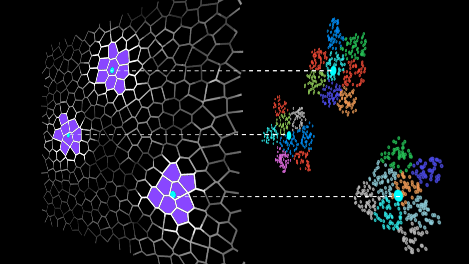
K-Means , BIRCH and Mean Shift are all commonly used clustering algorithms, and by no means are Data Scientists possessing the knowledge to implement these algorithms from scratch. Still, there is a necessity that Data Scientists understand the properties of each algorithm and their suitability to specific datasets.

For example, centroid based algorithms are favorable for high-density datasets where clusters can be clearly defined. In contrast, density-based algorithms such as DBSCAN(Density-based spatial clustering of application with Noise) are preferred when dealing with a noisy dataset.

In the context of sorting algorithms, Data Scientists come across data lakes and databases where traversing through elements to identify relationships is more efficient if the containing data is sorted.

Identifying library subroutines suitable for the dataset requires an understanding of various sorting algorithms preferred data structure types. Quicksort algorithms are favorable when working with arrays, but if data is presented as linked-list, then merge sort is more performant, especially in the case of a large dataset. Still, both use the divide and conquer strategy to sort data.

What’s a sorting algorithm?

The Sorting Problem is a well-known programming problem faced by Data Scientists and other software engineers. The primary purpose of the sorting problem is to arrange a set of objects in ascending or descending order. Sorting algorithms are sequential instructions executed to reorder elements within a list efficiently or array into the desired ordering.

What’s the purpose of sorting?

In the data realm, the structured organization of elements within a dataset enables the efficient traversing and quick lookup of specific elements or groups. At a macro level, applications built with efficient algorithms translate to simplicity introduced into our lives, such as navigation systems and search engines.

What’s insertion sort?

Insertion sort algorithm involves the sorted list created based on an iterative comparison of each element in the list with its adjacent element.

An index pointing at the current element indicates the position of the sort. At the beginning of the sort (index=0), the current value is compared to the adjacent value to the left. If the value is greater than the current value, no modifications are made to the list; this is also the case if the adjacent value and the current value are the same numbers. 

However, if the adjacent value to the left of the current value is lesser, then the adjacent value position is moved to the left, and only stops moving to the left if the value to the left of it is lesser.

The diagram illustrates the procedures taken in the insertion algorithm on an unsorted list. The list in the diagram below is sorted in ascending order (lowest to highest).

Algorithm Steps and Implementation (Python and JavaScript)

To order a list of elements in ascending order, the Insertion Sort algorithm requires the following operations:

• Begin with a list of unsorted elements.
• Iterate through the list of unsorted elements, from the first item to last.
• The current element is compared to the elements in all preceding positions to the left in each step.
• If the current element is less than any of the previously listed elements, it is moved one position to the left.

Implementation in Python

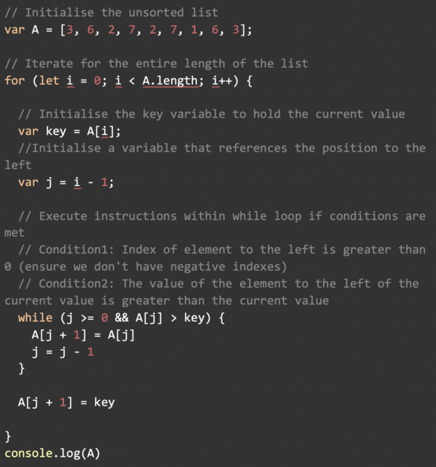
Implementation in JavaScript

Performance and Complexity

In the realm of computer science, ‘Big O notation is a strategy for measuring algorithm complexity. We won’t get too technical with Big O notation here. Still, it’s worth noting that computer scientists use this mathematical symbol to quantify algorithms according to their time and space requirements.

The Big O notation is a function that is defined in terms of the input. The letter ‘n’ often represents the size of the input to the function. Simply kept, n represents the number of elements in a list. In different scenarios, practitioners care about the worst-case, best-case, or average complexity of a function.

The worst-case (and average-case) complexity of the insertion sort algorithm is O(n²). Meaning that, in the worst case, the time taken to sort a list is proportional to the square of the number of elements in the list.

The best-case time complexity of insertion sort algorithm is O(n) time complexity. Meaning that the time taken to sort a list is proportional to the number of elements in the list; this is the case when the list is already in the correct order. There’s only one iteration in this case since the inner loop operation is trivial when the list is already in order.

Insertion sort is frequently used to arrange small lists. On the other hand, Insertion sort isn’t the most efficient method for handling large lists with numerous elements. Notably, the insertion sort algorithm is preferred when working with a linked list. And although the algorithm can be applied to data structured in an array, other sorting algorithms such as quicksort.

One of the simplest sorting methods is insertion sort, which involves building up a sorted list one element at a time. By inserting each unexamined element into the sorted list between elements that are less than it and greater than it. As demonstrated in this article, it’s a simple algorithm to grasp and apply in many languages.

By clearly describing the insertion sort algorithm, accompanied by a step-by-step breakdown of the algorithmic procedures involved. Data Scientists are better equipped to implement the insertion sort algorithm and explore other comparable sorting algorithms such as quicksort and bubble sort, and so on.

Algorithms may be a touchy subject for many Data Scientists. It may be due to the complexity of the topic. The word “algorithm” is sometimes associated with complexity. With the appropriate tools, training, and time, even the most complicated algorithms are simple to understand when you have enough time, information, and resources. Algorithms are fundamental tools used in data science and cannot be ignored.

Related resources

• GTC session: Data Science Ambassadors Discuss the Top 2024 Global AI and DS Trends (Presented by Z by HP)
• GTC session: Reducing the Cost of your Data Science Workloads on the Cloud
• GTC session: XGBoost is All You Need
• NGC Containers: Nvidia Clara Parabricks bamsort
• NGC Containers: MATLAB

About the Authors

Related posts

Streamline ETL Workflows with Nested Data Types in RAPIDS libcudf

Accelerated Vector Search: Approximating with RAPIDS RAFT IVF-Flat

Accelerated Data Analytics: Speed Up Data Exploration with RAPIDS cuDF

Merge Sort Explained: A Data Scientist’s Algorithm Guide

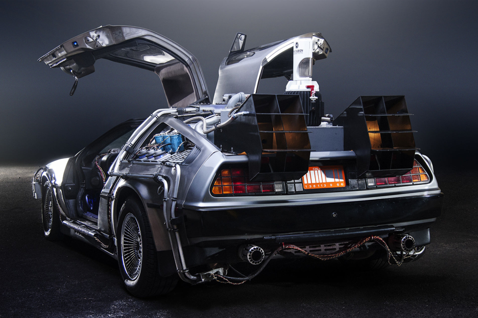
GPU-Accelerated Hierarchical DBSCAN with RAPIDS cuML – Let’s Get Back To The Future

Revolutionizing Graph Analytics: Next-Gen Architecture with NVIDIA cuGraph Acceleration

Efficient CUDA Debugging: Memory Initialization and Thread Synchronization with NVIDIA Compute Sanitizer

Analyzing the Security of Machine Learning Research Code

Comparing Solutions for Boosting Data Center Redundancy

Validating nvidia drive sim radar models.

• Running Time, Growth of Function and Asymptotic Notations

Best, Average and Worst case Analysis of Algorithms

• Amortized Analysis of Algorithms
• Calculating the running time of Algorithms
• Empirical way of calculating running time of Algorithms
• Understanding Recursion
• Tail Recursion
• Recurrence Relation
• Solving Recurrence Relations (Part I)
• Solving Recurrence Relations (Part II)
• Solving Recurrence Relations (Part III)

Before reading this article, I strongly recommend you to visit the following article.

• Running Time, Growth of Functions and Asymptotic Notations

Introduction

We all know that the running time of an algorithm increases (or remains constant in case of constant running time) as the input size ($n$) increases. Sometimes even if the size of the input is same, the running time varies among different instances of the input. In that case, we perform best, average and worst-case analysis. The best case gives the minimum time, the worst case running time gives the maximum time and average case running time gives the time required on average to execute the algorithm. I will explain all these concepts with the help of two examples - (i) Linear Search and (ii) Insertion sort.

Best Case Analysis

Consider the example of Linear Search where we search for an item in an array. If the item is in the array, we return the corresponding index, otherwise, we return -1. The code for linear search is given below.

Variable a is an array, n is the size of the array and item is the item we are looking for in the array. When the item we are looking for is in the very first position of the array, it will return the index immediately. The for loop runs only once. So the complexity, in this case, will be $O(1)$. This is the called the best case.

Consider another example of insertion sort. Insertion sort sorts the items in the input array in an ascending (or descending) order. It maintains the sorted and un-sorted parts in an array. It takes the items from the un-sorted part and inserts into the sorted part in its appropriate position. The figure below shows one snapshot of the insertion operation.

In the figure, items [1, 4, 7, 11, 53] are already sorted and now we want to place 33 in its appropriate place. The item to be inserted are compared with the items from right to left one-by-one until we found an item that is smaller than the item we are trying to insert. We compare 33 with 53 since 53 is bigger we move one position to the left and compare 33 with 11. Since 11 is smaller than 33, we place 33 just after 11 and move 53 one step to the right. Here we did 2 comparisons. It the item was 55 instead of 33, we would have performed only one comparison. That means, if the array is already sorted then only one comparison is necessary to place each item to its appropriate place and one scan of the array would sort it. The code for insertion operation is given below.

When items are already sorted, then the while loop executes only once for each item. There are total n items, so the running time would be $O(n)$. So the best case running time of insertion sort is $O(n)$.

The best case gives us a lower bound on the running time for any input. If the best case of the algorithm is $O(n)$ then we know that for any input the program needs at least $O(n)$ time to run. In reality, we rarely need the best case for our algorithm. We never design an algorithm based on the best case scenario.

Worst Case Analysis

In real life, most of the time we do the worst case analysis of an algorithm. Worst case running time is the longest running time for any input of size $n$.

In the linear search, the worst case happens when the item we are searching is in the last position of the array or the item is not in the array. In both the cases, we need to go through all $n$ items in the array. The worst case runtime is, therefore, $O(n)$. Worst case performance is more important than the best case performance in case of linear search because of the following reasons.

• The item we are searching is rarely in the first position. If the array has 1000 items from 1 to 1000. If we randomly search the item from 1 to 1000, there is 0.001 percent chance that the item will be in the first position.
• Most of the time the item is not in the array (or database in general). In which case it takes the worst case running time to run.

Similarly, in insertion sort, the worst case scenario occurs when the items are reverse sorted. The number of comparisons in the worst case will be in the order of $n^2$ and hence the running time is $O(n^2)$.

Knowing the worst-case performance of an algorithm provides a guarantee that the algorithm will never take any time longer.

Average Case Analysis

Sometimes we do the average case analysis on algorithms. Most of the time the average case is roughly as bad as the worst case. In the case of insertion sort, when we try to insert a new item to its appropriate position, we compare the new item with half of the sorted item on average. The complexity is still in the order of $n^2$ which is the worst-case running time.

It is usually harder to analyze the average behavior of an algorithm than to analyze its behavior in the worst case. This is because it may not be apparent what constitutes an “average” input for a particular problem. A useful analysis of the average behavior of an algorithm, therefore, requires a prior knowledge of the distribution of the input instances which is an unrealistic requirement. Therefore often we assume that all inputs of a given size are equally likely and do the probabilistic analysis for the average case.

If you're seeing this message, it means we're having trouble loading external resources on our website.

If you're behind a web filter, please make sure that the domains *.kastatic.org and *.kasandbox.org are unblocked.

To log in and use all the features of Khan Academy, please enable JavaScript in your browser.

Computer science theory

Course: computer science theory   >   unit 1.

• Challenge: implement swap
• Selection sort pseudocode
• Challenge: Find minimum in subarray
• Challenge: implement selection sort

Analysis of selection sort

• Project: Selection sort visualizer
• In the first call of indexOfMinimum , it has to look at every value in the array, and so the loop body in indexOfMinimum runs 8 times.
• In the second call of indexOfMinimum , it has to look at every value in the subarray from indices 1 to 7, and so the loop body in indexOfMinimum runs 7 times.
• In the third call, it looks at the subarray from indices 2 to 7; the loop body runs 6 times.
• In the fourth call, it looks at the subarray from indices 3 to 7; the loop body runs 5 times.
• In the eighth and final call of indexOfMinimum , the loop body runs just 1 time.

Side note: Computing summations from 1 to n ‍  

• Add the smallest and the largest number.
• Multiply by the number of pairs.

Asymptotic running-time analysis for selection sort

• The running time for all the calls to indexOfMinimum .
• The running time for all the calls to swap .
• The running time for the rest of the loop in the selectionSort function.

Want to join the conversation?

• Upvote Button navigates to signup page
• Downvote Button navigates to signup page
• Flag Button navigates to signup page