what is analysis excel

Use the Analysis ToolPak to perform complex data analysis

If you need to develop complex statistical or engineering analyses, you can save steps and time by using the Analysis ToolPak. You provide the data and parameters for each analysis, and the tool uses the appropriate statistical or engineering macro functions to calculate and display the results in an output table. Some tools generate charts in addition to output tables.

The data analysis functions can be used on only one worksheet at a time. When you perform data analysis on grouped worksheets, results will appear on the first worksheet and empty formatted tables will appear on the remaining worksheets. To perform data analysis on the remainder of the worksheets, recalculate the analysis tool for each worksheet.

The Analysis ToolPak includes the tools described in the following sections. To access these tools, click Data Analysis in the Analysis group on the Data tab. If the Data Analysis command is not available, you need to load the Analysis ToolPak add-in program.

Load and activate the Analysis ToolPak

Click the File tab, click Options , and then click the Add-Ins category.

In the Manage box, select Excel Add-ins and then click Go .

If you're using Excel for Mac, in the file menu go to Tools > Excel Add-ins.

In the Add-Ins box, check the Analysis ToolPak check box, and then click OK .

If Analysis ToolPak is not listed in the Add-Ins available box, click Browse to locate it.

If you are prompted that the Analysis ToolPak is not currently installed on your computer, click Yes to install it.

Note: To include Visual Basic for Application (VBA) functions for the Analysis ToolPak, you can load the Analysis ToolPak - VBA Add-in the same way that you load the Analysis ToolPak. In the Add-ins available box, select the Analysis ToolPak - VBA check box.

The Anova analysis tools provide different types of variance analysis. The tool that you should use depends on the number of factors and the number of samples that you have from the populations that you want to test.

Anova: Single Factor

This tool performs a simple analysis of variance on data for two or more samples. The analysis provides a test of the hypothesis that each sample is drawn from the same underlying probability distribution against the alternative hypothesis that underlying probability distributions are not the same for all samples. If there are only two samples, you can use the worksheet function T . TEST . With more than two samples, there is no convenient generalization of T . TEST , and the Single Factor Anova model can be called upon instead.

Anova: Two-Factor with Replication

This analysis tool is useful when data can be classified along two different dimensions. For example, in an experiment to measure the height of plants, the plants may be given different brands of fertilizer (for example, A, B, C) and might also be kept at different temperatures (for example, low, high). For each of the six possible pairs of {fertilizer, temperature}, we have an equal number of observations of plant height. Using this Anova tool, we can test:

Whether the heights of plants for the different fertilizer brands are drawn from the same underlying population. Temperatures are ignored for this analysis.

Whether the heights of plants for the different temperature levels are drawn from the same underlying population. Fertilizer brands are ignored for this analysis.

Whether having accounted for the effects of differences between fertilizer brands found in the first bulleted point and differences in temperatures found in the second bulleted point, the six samples representing all pairs of {fertilizer, temperature} values are drawn from the same population. The alternative hypothesis is that there are effects due to specific {fertilizer, temperature} pairs over and above the differences that are based on fertilizer alone or on temperature alone.

Anova: Two-Factor Without Replication

This analysis tool is useful when data is classified on two different dimensions as in the Two-Factor case With Replication. However, for this tool it is assumed that there is only a single observation for each pair (for example, each {fertilizer, temperature} pair in the preceding example).

Correlation

The CORREL and PEARSON worksheet functions both calculate the correlation coefficient between two measurement variables when measurements on each variable are observed for each of N subjects. (Any missing observation for any subject causes that subject to be ignored in the analysis.) The Correlation analysis tool is particularly useful when there are more than two measurement variables for each of N subjects. It provides an output table, a correlation matrix, that shows the value of CORREL (or PEARSON ) applied to each possible pair of measurement variables.

The correlation coefficient, like the covariance, is a measure of the extent to which two measurement variables "vary together." Unlike the covariance, the correlation coefficient is scaled so that its value is independent of the units in which the two measurement variables are expressed. (For example, if the two measurement variables are weight and height, the value of the correlation coefficient is unchanged if weight is converted from pounds to kilograms.) The value of any correlation coefficient must be between -1 and +1 inclusive.

You can use the correlation analysis tool to examine each pair of measurement variables to determine whether the two measurement variables tend to move together — that is, whether large values of one variable tend to be associated with large values of the other (positive correlation), whether small values of one variable tend to be associated with large values of the other (negative correlation), or whether values of both variables tend to be unrelated (correlation near 0 (zero)).

The Correlation and Covariance tools can both be used in the same setting, when you have N different measurement variables observed on a set of individuals. The Correlation and Covariance tools each give an output table, a matrix, that shows the correlation coefficient or covariance, respectively, between each pair of measurement variables. The difference is that correlation coefficients are scaled to lie between -1 and +1 inclusive. Corresponding covariances are not scaled. Both the correlation coefficient and the covariance are measures of the extent to which two variables "vary together."

The Covariance tool computes the value of the worksheet function COVARIANCE.P for each pair of measurement variables. (Direct use of COVARIANCE.P rather than the Covariance tool is a reasonable alternative when there are only two measurement variables, that is, N=2.) The entry on the diagonal of the Covariance tool's output table in row i, column i is the covariance of the i-th measurement variable with itself. This is just the population variance for that variable, as calculated by the worksheet function VAR . P .

You can use the Covariance tool to examine each pair of measurement variables to determine whether the two measurement variables tend to move together — that is, whether large values of one variable tend to be associated with large values of the other (positive covariance), whether small values of one variable tend to be associated with large values of the other (negative covariance), or whether values of both variables tend to be unrelated (covariance near 0 (zero)).

Descriptive Statistics

The Descriptive Statistics analysis tool generates a report of univariate statistics for data in the input range, providing information about the central tendency and variability of your data.

Exponential Smoothing

The Exponential Smoothing analysis tool predicts a value that is based on the forecast for the prior period, adjusted for the error in that prior forecast. The tool uses the smoothing constant a , the magnitude of which determines how strongly the forecasts respond to errors in the prior forecast.

Note: Values of 0.2 to 0.3 are reasonable smoothing constants. These values indicate that the current forecast should be adjusted 20 percent to 30 percent for error in the prior forecast. Larger constants yield a faster response but can produce erratic projections. Smaller constants can result in long lags for forecast values.

F-Test Two-Sample for Variances

The F-Test Two-Sample for Variances analysis tool performs a two-sample F-test to compare two population variances.

For example, you can use the F-Test tool on samples of times in a swim meet for each of two teams. The tool provides the result of a test of the null hypothesis that these two samples come from distributions with equal variances, against the alternative that the variances are not equal in the underlying distributions.

The tool calculates the value f of an F-statistic (or F-ratio). A value of f close to 1 provides evidence that the underlying population variances are equal. In the output table, if f < 1 "P(F <= f) one-tail" gives the probability of observing a value of the F-statistic less than f when population variances are equal, and "F Critical one-tail" gives the critical value less than 1 for the chosen significance level, Alpha. If f > 1, "P(F <= f) one-tail" gives the probability of observing a value of the F-statistic greater than f when population variances are equal, and "F Critical one-tail" gives the critical value greater than 1 for Alpha.

Fourier Analysis

The Fourier Analysis tool solves problems in linear systems and analyzes periodic data by using the Fast Fourier Transform (FFT) method to transform data. This tool also supports inverse transformations, in which the inverse of transformed data returns the original data.

The Histogram analysis tool calculates individual and cumulative frequencies for a cell range of data and data bins. This tool generates data for the number of occurrences of a value in a data set.

For example, in a class of 20 students, you can determine the distribution of scores in letter-grade categories. A histogram table presents the letter-grade boundaries and the number of scores between the lowest bound and the current bound. The single most-frequent score is the mode of the data.

Tip: In Excel 2016, you can now create a histogram or Pareto chart.

Moving Average

The Moving Average analysis tool projects values in the forecast period, based on the average value of the variable over a specific number of preceding periods. A moving average provides trend information that a simple average of all historical data would mask. Use this tool to forecast sales, inventory, or other trends. Each forecast value is based on the following formula.

N is the number of prior periods to include in the moving average

A j is the actual value at time j

F j is the forecasted value at time j

Random Number Generation

The Random Number Generation analysis tool fills a range with independent random numbers that are drawn from one of several distributions. You can characterize the subjects in a population with a probability distribution. For example, you can use a normal distribution to characterize the population of individuals' heights, or you can use a Bernoulli distribution of two possible outcomes to characterize the population of coin-flip results.

Rank and Percentile

The Rank and Percentile analysis tool produces a table that contains the ordinal and percentage rank of each value in a data set. You can analyze the relative standing of values in a data set. This tool uses the worksheet functions RANK.EQ and PERCENTRANK.INC . If you want to account for tied values, use the RANK.EQ function, which treats tied values as having the same rank, or use the RANK. AVG function, which returns the average rank for the tied values.

The Regression analysis tool performs linear regression analysis by using the "least squares" method to fit a line through a set of observations. You can analyze how a single dependent variable is affected by the values of one or more independent variables. For example, you can analyze how an athlete's performance is affected by such factors as age, height, and weight. You can apportion shares in the performance measure to each of these three factors, based on a set of performance data, and then use the results to predict the performance of a new, untested athlete.

The Regression tool uses the worksheet function LINEST .

The Sampling analysis tool creates a sample from a population by treating the input range as a population. When the population is too large to process or chart, you can use a representative sample. You can also create a sample that contains only the values from a particular part of a cycle if you believe that the input data is periodic. For example, if the input range contains quarterly sales figures, sampling with a periodic rate of four places the values from the same quarter in the output range.

The Two-Sample t-Test analysis tools test for equality of the population means that underlie each sample. The three tools employ different assumptions: that the population variances are equal, that the population variances are not equal, and that the two samples represent before-treatment and after-treatment observations on the same subjects.

For all three tools below, a t-Statistic value, t, is computed and shown as "t Stat" in the output tables. Depending on the data, this value, t, can be negative or nonnegative. Under the assumption of equal underlying population means, if t < 0, "P(T <= t) one-tail" gives the probability that a value of the t-Statistic would be observed that is more negative than t. If t >=0, "P(T <= t) one-tail" gives the probability that a value of the t-Statistic would be observed that is more positive than t. "t Critical one-tail" gives the cutoff value, so that the probability of observing a value of the t-Statistic greater than or equal to "t Critical one-tail" is Alpha.

"P(T <= t) two-tail" gives the probability that a value of the t-Statistic would be observed that is larger in absolute value than t. "P Critical two-tail" gives the cutoff value, so that the probability of an observed t-Statistic larger in absolute value than "P Critical two-tail" is Alpha.

t-Test: Paired Two Sample For Means

You can use a paired test when there is a natural pairing of observations in the samples, such as when a sample group is tested twice — before and after an experiment. This analysis tool and its formula perform a paired two-sample Student's t-Test to determine whether observations that are taken before a treatment and observations taken after a treatment are likely to have come from distributions with equal population means. This t-Test form does not assume that the variances of both populations are equal.

Note: Among the results that are generated by this tool is pooled variance, an accumulated measure of the spread of data about the mean, which is derived from the following formula.

t-Test: Two-Sample Assuming Equal Variances

This analysis tool performs a two-sample student's t-Test. This t-Test form assumes that the two data sets came from distributions with the same variances. It is referred to as a homoscedastic t-Test. You can use this t-Test to determine whether the two samples are likely to have come from distributions with equal population means.

t-Test: Two-Sample Assuming Unequal Variances

This analysis tool performs a two-sample student's t-Test. This t-Test form assumes that the two data sets came from distributions with unequal variances. It is referred to as a heteroscedastic t-Test. As with the preceding Equal Variances case, you can use this t-Test to determine whether the two samples are likely to have come from distributions with equal population means. Use this test when there are distinct subjects in the two samples. Use the Paired test, described in the follow example, when there is a single set of subjects and the two samples represent measurements for each subject before and after a treatment.

The following formula is used to determine the statistic value t .

The following formula is used to calculate the degrees of freedom, df. Because the result of the calculation is usually not an integer, the value of df is rounded to the nearest integer to obtain a critical value from the t table. The Excel worksheet function T . TEST uses the calculated df value without rounding, because it is possible to compute a value for T . TEST with a noninteger df. Because of these different approaches to determining the degrees of freedom, the results of T . TEST and this t-Test tool will differ in the Unequal Variances case.

The z-Test: Two Sample for Means analysis tool performs a two sample z-Test for means with known variances. This tool is used to test the null hypothesis that there is no difference between two population means against either one-sided or two-sided alternative hypotheses. If variances are not known, the worksheet function Z . TEST should be used instead.

When you use the z-Test tool, be careful to understand the output. "P(Z <= z) one-tail" is really P(Z >= ABS(z)), the probability of a z-value further from 0 in the same direction as the observed z value when there is no difference between the population means. "P(Z <= z) two-tail" is really P(Z >= ABS(z) or Z <= -ABS(z)), the probability of a z-value further from 0 in either direction than the observed z-value when there is no difference between the population means. The two-tailed result is just the one-tailed result multiplied by 2. The z-Test tool can also be used for the case where the null hypothesis is that there is a specific nonzero value for the difference between the two population means. For example, you can use this test to determine differences between the performances of two car models.

Need more help?

You can always ask an expert in the Excel Tech Community or get support in Communities .

Create a histogram in Excel 2016

Create a Pareto chart in Excel 2016

Load the Analysis ToolPak in Excel

ENGINEERING functions (reference)

Overview of formulas in Excel

How to avoid broken formulas

Find and correct errors in formulas

Excel keyboard shortcuts and function keys

Excel functions (alphabetical)

Excel functions (by category)

Want more options?

Explore subscription benefits, browse training courses, learn how to secure your device, and more.

Microsoft 365 subscription benefits

Microsoft 365 training

Microsoft security

Accessibility center

Communities help you ask and answer questions, give feedback, and hear from experts with rich knowledge.

Ask the Microsoft Community

Microsoft Tech Community

Windows Insiders

Microsoft 365 Insiders

Was this information helpful?

Thank you for your feedback.

How-To Geek

7 excel data analysis features you have to try.

Your changes have been saved

Email Is sent

Please verify your email address.

You’ve reached your account maximum for followed topics.

Microsoft Office Now Plays Better With LibreOffice

Netflix is starting to kill off its basic plan, 20+ surprisingly good-looking games you can play on a potato gaming pc, quick links, quick analysis for helpful tools, analyze data for asking questions, charts and graphs for visual analysis, sort and filter for easier viewing, functions for creating formulas, conditional formatting for spotting data fast, pivot tables for complex data.

No matter what you use Excel for, whether business financials or a personal budget, the tool's data analysis features can help you make sense of your data. Here are several Excel features for data analysis and how they can help.

When you aren't quite sure of the best way to display your data or if you're a new Excel user, the Quick Analysis feature is essential. With it, you simply select your data and view various analysis tools provided by Excel.

Related: How to Use Excel's "Quick Analysis" to Visualize Data

Select the data you want to analyze. You'll see a small button appear in the bottom corner of the selected cells. Click this Quick Analysis button, and you'll see several options to review.

Choose "Formatting" to look through ways to use conditional formatting. You can also select "Charts" to see the graphs Excel recommends for the data, "Totals" for calculations using functions and formulas, "Tables" to create a table or pivot table, and "Sparklines" to insert tiny charts for your data.

After you pick a tool, hover your cursor over the options to see previews. For example, if you select Formatting, hover your cursor over Data Bars, Color Scale, Icon Set, or another option to see how your data would look.

Simply choose the tool you want and you're in business.

Another helpful built-in feature in Excel is the Analyze Data tool . With it, you can ask questions about your data and see suggested questions and answers. You can also quickly insert items like charts and tables.

Select your data, go to the Home tab, and click "Analyze Data" in the Analysis section of the ribbon.

You'll see a sidebar open on the right. At the top, pop a question into the search box. Alternatively, you can choose a question in the Not Sure What to Ask section or scroll through the sidebar for recommendations.

If you see a table or chart in the list you want to use, select "Insert Chart" or "Insert PivotTable" to add it to your sheet with a click.

Analyze Data sidebar with insert options

As mentioned above, charts make great visual analysis tools. Luckily, Excel offers many types of graphs and charts, each with robust customization options.

Related: How to Choose a Chart to Fit Your Data in Microsoft Excel

Select your data and go to the Insert tab. You can choose "Recommended Charts" in the Charts section of the ribbon to see which graph Excel believes fits your data best .

You can also pick "All Charts" in the Recommended Charts window or choose a specific chart type in that same section of the ribbon if you know which kind of visual you want.

When you pick a chart type, you'll see it appear in your sheet with your data already inserted. From there, you can select the graph and use the Chart Design tab, Format Chart Area sidebar, and chart buttons (Windows only) to customize the chart and the data in it.

Chart Design tab and customization buttons on Windows

For more, check out our how-tos for making graphs in Excel . We can help you create a pie chart , waterfall chart , funnel chart , combo chart , and more.

When you want to analyze particular data in your Excel sheet, the sort and filter options help you accomplish this.

You may have columns of data that you want to sort alphabetically , numerically, by color, or using a particular value.

Select the data, go to the Home tab, and open the Sort & Filter drop-down menu. You can choose a quick sort option or "Custom Sort" to pick a certain value.

Along with sorting the data, you can use filters to see only the data you need at the time. Select the data, open the same Sort & Filter menu, and pick "Filter."

You'll see filter buttons at the top of each column. Select a button to filter that column by color or number. You can also use the checkboxes at the bottom of the pop-up window.

To clear a filter when you finish, select the filter button and choose "Clear Filter." To turn off filtering altogether, return to the Sort & Filter menu on the Home tab and deselect "Filter."

Excel's functions are fantastic tools for creating formulas to manipulate, change, convert, combine, split, and perform many more actions with your data. When it comes to analyzing data, here are just a handful of functions that can come in handy.

The IF and IFS functions are invaluable in Excel. You can perform a test and return a true or false result based on criteria. IFS lets you use multiple conditions. IF and IFS are also useful when you combine them with other functions.

COUNTIF and COUNTIFS

The COUNTIF and COUNTIFS functions count the number of cells containing data that meets certain criteria. COUNTIFS lets you use multiple conditions.

SUMIF and SUMIFS

The SUMIF and SUMIFS math functions add values in cells based on criteria. SUMIFS lets you use multiple conditions.

XLOOKUP, VLOOKUP, and HLOOKUP

The XLOOKUP , VLOOKUP , and HLOOKUP functions help you locate specific data in your sheet. Use XLOOKUP to find data in any direction, VLOOKUP to find data vertically, or HLOOKUP to find data horizontally. XLOOKUP is the most versatile of the three and is an extremely helpful function.

With the UNIQUE lookup function, you can obtain a list of only the unique values from your data set.

Conditional formatting is a favorite feature for sure. Once you set it up, you can spot specific data quickly, making data analysis go faster.

Select your data, go to the Home tab, and click the Conditional Formatting drop-down menu. You'll see several ways to format your data, such as highlighting cells greater or less than a specific value or showing the top or bottom 10 items.

Conditional Formatting highlight options

You can also use conditional formatting to find duplicate data , insert color scales for things like heat maps, create data bars for color indicators, and use icon sets for handy visuals like shapes and arrows.

Additionally, you can create a custom rule, apply more than one rule at a time, and clear rules you no longer want.

One of the most powerful Excel tools for data analysis is the pivot table . With it, you can arrange, group, summarize, and calculate data using an interactive table.

Related: How to Use Pivot Tables to Analyze Excel Data

Select the data you want to add to a pivot table and head to the Insert tab. Similar to charts, you can review Excel's suggestions by selecting "Recommended PivotTables" in the Tables section of the ribbon. Alternatively, you can create one from scratch by clicking the PivotTable button in that same section.

You'll then see a placeholder added to your workbook for the pivot table. On the right, use the PivotTable Fields sidebar to customize the contents of the table.

Use the checkboxes to choose which data to include and then the areas below to apply filters and designate the rows and columns. You can also use the PivotTable Analyze tab.

Because pivot tables can be a little intimidating when you get started, check out our complete tutorial for creating a pivot table in Excel .

Hopefully, one or more of these Excel data analysis features will help you with your next review or evaluation task.

Microsoft Office
Microsoft Excel

List Your Business in Our Directory Now! →

Business Directory
Excel Data Analysis

What If Analysis Excel

Written by: Bill Whitman

Last updated: May 20, 2023

If you’re looking to analyze various scenarios and their outcomes in Microsoft Excel, then What-if analysis is the tool you need. This feature allows you to compare different variables, allowing you to make informed decisions based on the results of each model you create. What-if analysis provides an excellent solution for those looking to understand the implications of different financial or organizational decisions. In this blog post, we will be explaining everything you need to know about What If Analysis Excel and how you can use it to make your business more efficient and profitable.

What Is What-If Analysis Excel?

Microsoft Excel’s What-if analysis is a tool that allows you to check and analyze different scenarios and how they may impact a business, financial investment, or project. What-if analysis helps you compare various data sets and make better financial decisions based on the insights you gain.

Types of What-If Analysis

Data Table is a What-if analysis tool that helps you calculate different outcomes. With the Data Table option, you can create new values for the variables and observe how the result changes. Data Table is best used to test and compare multiple outcomes and scenarios.

Goal Seek is a What-if analysis toll that helps you determine a desired outcome by changing one of the initial values given. Here, Excel works backward by starting with an unknown value that you want to achieve and calculates the input value required to meet that objective. Goal Seek is best used when you want to attain a specific target—sales growth, projected revenue, etc.

Scenario Manager

Scenario Manager is a What-if analysis tool that allows you to create and compare different scenarios by playing with the variables. The scenarios are the different outcomes that result from the variation of values in the variables. Suppose you are seeking a new investment opportunity. In that case, this tool allows you to analyze different financial options based on the different variables that influence the outcome, such as investment amount, exchange rate, time horizon, and projected return on investment.

Steps to Use What-If Analysis Excel

Step 1: identify the objective.

The first step is to identify the objective of the analysis. You need to know the specific problem you are trying to solve and what information you aim to obtain. This information will guide the type of What-if analysis tool you use.

Step 2: Define the Variables

The next step is to define the variables that affect the outcome of the analysis and the range of values they can assume. These variables may include expenditure, sales, revenue, or any other relevant metric.

Step 3: Create the Model

The model is the framework that will guide the What-if analysis process. Here, you enter the equations and formulas that will generate the output based on the input. The equations must be based on the variables identified in step two. You can use Excel’s built-in formulas, such as those under the Financial function, for this step.

Step 4: Determine Your Input Cells

You need to identify the input cells for the analysis. These are the cells that you will change to perform the analysis and the range of values they can assume. These cells will vary, depending on the type of What-if analysis tool you are using.

Step 5: Execute What-If Analysis

At this point, you can use any of the What-if analysis tools highlighted in this blog post to perform your analysis. The goal is to achieve the desired outcome by varying the input values and observing how the output values change.

In conclusion, What-if Analysis Excel is a powerful tool that can help you improve your financial decision-making process. With Data Table, Goal Seek, and Scenario Manager features, you can quickly and easily analyze different scenarios and their potential impact on your business. So next time you need to perform a What-if analysis in Microsoft Excel, follow these five easy steps, and you will be well on your way to making data-driven decisions that can benefit your business.

Tips for using What-if Analysis Excel

Keep it simple.

When creating the model, start with basic formulas and relevant variables. It’s better to use a generic model that can easily be modified than to have a complex model that is hard to understand or modify in the future.

Label Your Input and Output Values

Labeling the input and output values helps in identifying them quickly. It also ensures you don’t modify the wrong cells during the analysis process. Use the Name Box or Formula Auditing Toolbar to label your cells.

Tables help you format and visualize your data better and ensure that your input and output values stay organized. You can convert your data range into a table by pressing Ctrl+T or going to the ‘Insert’ tab, then clicking ‘Table.’

Use Different Colors for Different Scenarios

When using the Scenario Manager, use different colors to represent different scenarios. This will help you keep track of the changes you’re making quickly and easily.

Test Your Models

Before making any critical decisions based on the analysis, test your models using realistic data. Ensure the accuracy of your data and verify the results of your analysis. Double-check your equations and formulas too.

Benefits of What-If Analysis Excel

What-If Analysis in Excel is a versatile tool that provides several benefits, including:

Improved Decision Making

What-if analysis helps you make informed decisions by modeling and comparing several scenarios and observing their impact on the outcome. You can analyze the impact on costs, revenue, and other relevant metrics, giving you a better overview of what to expect.

Time and Cost-Efficient

The What-if analysis feature is quick and efficient. You can run several scenarios and get an outcome in real-time; hence one doesn’t have to spend a lot of time analyzing data manually.

Helps Reduce Business Risk

What-if analysis helps businesses to make predictions based on real data, which helps mitigate business risks while providing a chance to calculate alternatives without incurring actual risk.

Explore What-If Situations Easily

You can quickly and easily explore several ‘What-If’ situations with the What-if analysis tool, which allows you to test and evaluate different alternatives without necessarily investing in them.

Final thoughts

What-If Analysis Excel is a powerful tool that can offer vital insights into the financial and strategic decisions of a business or project. Whether you are comparing sales scenarios, testing investment strategies, or estimating the impact of a new business model, Microsoft Excel’s What-If Analysis feature gives you the ability to make projections based on real data. Follow the tips outlined in this post to ensure the accuracy and reliability of your analysis. Remember, the more accurate your input, the more reliable your output.

Here are some common questions regarding What If Analysis Excel:

Can I undo What-if analysis changes made to my spreadsheet?

Yes, you can undo or revert to the original values of the cells that you changed during What-If Analysis by clicking on “Undo” or “Revert” under the “What-If Analysis” tab on the Ribbon.

Does What-if analysis feature work with all versions of Excel?

Yes, the What-If Analysis feature is available in all versions of Microsoft Excel.

How do I input formulas for a What-if analysis?

You can input formulas for a What-If analysis by selecting the cell where you want the formula to be and typing in the formula. Alternatively, you can use the Formula Builder or Function Wizard in Microsoft Excel to input your formulas.

Can I add multiple scenarios to my model?

Yes, the Scenario Manager allows you to add, delete, and modify different scenarios. You can use different variables and input values for each scenario to compare the outcomes.

Can I print out the results of my What-if analysis?

Yes, you can print out the results of your What-If Analysis by selecting the cells containing the input and output values and clicking on “Print” under the “File” tab. Alternatively, you can copy and paste the values into a Word document or other format.

Featured Companies

Learn powerpoint.

Explore the world of Microsoft PowerPoint with LearnPowerpoint.io, where we provide tailored tutorials and valuable tips to transform your presentation skills and clarify PowerPoint for enthusiasts and professionals alike.

Your ultimate guide to mastering Microsoft Word! Dive into our extensive collection of tutorials and tips designed to make Word simple and effective for users of all skill levels.

Resultris Marketing

Boost your brand's online presence with Resultris Content Marketing Subscriptions. Enjoy high-quality, on-demand content marketing services to grow your business.

How to Do Calculations in Excel

How to Convert Military Time to Standard Time in Excel

How to Use SUMIF in Excel

How to Filter Columns in Excel

How to Do Bullet Points in Excel

How to Use Advanced Filter in Excel

How to Adjust Column Width in Excel

How to Change Axis Labels in Excel

How to Divide Excel Cells

Excel - What-if Analysis

Excel -, what-if analysis, excel what-if analysis.

Excel: What-if Analysis

Lesson 29: what-if analysis.

/en/excel/doing-more-with-pivottables/content/

Introduction

Excel includes powerful tools to perform complex mathematical calculations, including what-if analysis . This feature can help you experiment and answer questions with your data, even when the data is incomplete. In this lesson, you will learn how to use a what-if analysis tool called Goal Seek .

Optional: Download our practice workbook .

Watch the video below to learn more about what-if analysis and Goal Seek.

Whenever you create a formula or function in Excel, you put various parts together to calculate a result . Goal Seek works in the opposite way: It lets you start with the desired result , and it calculates the input value that will give you that result. We'll use a few examples to show how to use Goal Seek.

To use Goal Seek (example 1):

Let's say you're enrolled in a class. You currently have a grade of 65, and you need at least a 70 to pass the class. Luckily, you have one final assignment that might be able to raise your average. You can use Goal Seek to find out what grade you need on the final assignment to pass the class.

In the image below, you can see that the grades on the first four assignments are 58 , 70 , 72 , and 60 . Even though we don't know what the fifth grade will be, we can write a formula—or function—that calculates the final grade. In this case, each assignment is weighted equally, so all we have to do is average all five grades by typing =AVERAGE(B2:B6) . Once we use Goal Seek, cell B6 will show us the minimum grade we'll need to make on that assignment.

the average function being used to average the other class grades

A dialog box will appear with three fields. The first field, Set cell: , will contain the desired result. In our example, cell B7 is already selected. The second field, To value: , is the desired result. In our example, we'll enter 70 because we need to earn at least that to pass the class. The third field, B y changing cell: , is the cell where Goal Seek will place its answer. In our example, we'll select cell B6 because we want to determine the grade we need to earn on the final assignment.

setting parameters in the goal seek dialog box

To use Goal Seek (example 2):

Let's say you're planning an event and want to invite as many people as you can without exceeding a budget of $500. We can use Goal Seek to figure out how many people to invite. In our example below, cell B5 contains the formula =B2+B3*B4 to calculate the total cost of a room reservation, plus the cost per person.

A dialog box will appear with three fields. The first field, Set cell: , will contain the desired result. In our example, cell B5 is already selected. The second field, To value: , is the desired result. In our example, we'll enter 500 because we only want to spend $500. The third field, By changing cell: , is the cell where Goal Seek will place its answer. In our example, we'll select cell B4 because we want to know how many guests we can invite without spending more than $500.

The dialog box will tell you if Goal Seek was able to find a solution. Click OK .

the value in cell B4 (18) determined by Goal Seek

As you can see in the example above, some situations will require the answer to be a whole number. If Goal Seek gives you a decimal, you'll need to round up or down , depending on the situation.

Other types of what-if analysis

For more advanced projects, you may want to consider the other types of what-if analysis: scenarios and data tables . Instead of starting from the desired result and working backward, like with Goal Seek, these options allow you to test multiple values and see how the results change.

For more information on scenarios, read this article from Microsoft.

For more information on data tables, read this article from Microsoft.

Open our practice workbook .
Click the Challenge tab in the bottom-left of the workbook.
In cell B8 , create a function that calculates the average of the sales in B2:B7 .
The workbook shows Dave's monthly sales amounts for the first half of the year. If he reaches a $200,000 mid-year average, he will receive a 5% bonus. Use Goal Seek to find how much he needs to sell in June in order to make the $200,000 average.

/en/excel/what-is-office-365/content/

Ablebits blog
Excel tips & how-to

Excel Quick Analysis tool with examples

In this tutorial, you will learn how to simplify your common tasks and gain new insights with the Excel Quick Analysis tool.

Microsoft Excel is a powerful spreadsheet application that can handle various types of data, but sometimes, you need to quickly get insights without diving deep into complex functions and formulas. That's where the Quick Analysis tool comes into play. In this article, we'll explore what the Quick Analysis tool is, where to find it in Excel, how to enable it, and how to use it to perform common tasks with just a few clicks.

What is Excel Quick Analysis tool?

Where is the Quick Analysis tool in Excel?

Unlike traditional Excel features found on the ribbon or menus, the Quick Analysis tool operates in a more discreet manner.

To access Quick Analysis in Excel, highlight a range of cells in your worksheet. In the bottom-right corner of the selected range, you'll notice a small icon that looks like a small box with a lightning bolt. This is the Quick Analysis button . Clicking this button will open the menu, where you can choose from different categories of features.

If the Quick Analysis button does not show up after selecting your data, use the Ctrl + Q shortcut to activate it.

How to enable / disable Quick Analysis tool in Excel?

In some cases, you may not see the Quick Analysis icon when you select your data. If this happens, most likely this feature is disabled in your Excel, and you need to enable it manually in the Excel options. Here's how:

Click on the File tab on the left side of the Excel ribbon.
Select Options at the bottom of the left-hand panel.
In the Excel Options window, navigate to the General section and tick the checkbox labeled Show Quick Analysis options on selection .
Click OK to save your preferences.

Now, the Quick Analysis button should be visible whenever you select a range of data, providing quick access to its functionality.

Tip. To prevent the Quick Analysis tool from appearing every time you select data and interrupting your workflow, simply uncheck the Show Quick Analysis Options on Selection tick box to toggle it off.

How to use Quick Analysis tool in Excel

Using the Quick Analysis tool is an intuitive and user-friendly process. The steps are:

Begin by selecting the data you wish to analyze. This could be a table, a list of numbers or text strings, or any relevant dataset.
Shift your focus to the bottom-right corner of the selected range and click the Quick Analysis button. In case the icon isn't visible, press Ctrl + Q to summon it.
In the Quick Analysis menu, you'll discover a few categories of features tailored for your data analysis needs. Hover over a specific option to see a preview of how it will transform your data. When you click on the option, it will be immediately applied to your data.

Below is an overview of the 5 main categories within the Quick Analysis tool. For those who prefer to navigate apps without using the mouse, keyboard shortcuts are available for each category.

This category allows you to enhance data visualization by applying conditional formatting . The available options depend on the data type you’ve selected:

For numeric data , you can use Data Bars, Icon Sets, Greater Than, and Top 10%, to highlight the relevant numbers in your dataset.
For text values , you’ll have Highlight Duplicates, Unique Values, Cells That Contain, or Exact Match to identify and filter your data based on text criteria.
For dates , you’ll be able to highlight the ones occurring Last Month, Last Week as well as Greater Than, Less Than, or Equal To a particular date.

Apart from the traditional ways to create charts in Excel , you can also use the Quick Analysis tool to insert a graph. While Quick Analysis provides a limited range of options, it intelligently suggests the most suitable chart types and makes the process faster.

Based on your selected data, Excel’s Quick Analysis tool will display the chart types that are the best fit to represent your data graphically and help you visualize the patterns, trends, and relationships. You can hover over each graph type to see a preview of how it would look like in your worksheet.

If the chart type you are looking for is not there, click on the More Charts option, which will open the Insert Chart dialog box, where you can select from a variety of other graph types, such as scatter plots, histograms, radar charts, and others.

With Totals, you can easily calculate and display various summary statistics for your data, such as sum, average, count, percentage total, and running total.

Depending on the type and format of the data in the selected range, you will see different options for applying totals. For example, if you only have text data, the only option available will be Count , which shows the number of cells with text values.

Quick Analysis Totals to calculate summary statistics

Tables / PivotTables

Quick Analysis options for tables and pivot tables

Sparklines are a great way to show data trends in a compact and elegant way. Insert these tiny in-cell charts to visualize patterns within your dataset, choosing from three types: Line, Column, or Win/Loss.

Examples of using Quick Analysis tools in Excel

Now let’s explorer some practical examples of how you can use the Quick Analysis tools in Excel to analyze your data faster and easier. We will use a sample dataset of monthly sales of different items.

Change a regular range into Excel table

The first thing we do is to turn our sample dataset into an Excel table. Transforming a regular data range into a fully-functional table offers numerous advantages, including automatic expansion for new records, meaning that all the adjustments you make for the current data will be automatically applied to new records without you having to do anything extra.

Here's how you can quickly create a table using the Excel Quick Analysis tool:

Select your data.
Click the Quick Analysis button or press the Ctrl + Q shortcut.
Within the Quick Analysis menu, navigate to the Tables category and select Table .

Using Quick Analysis to convert a range into an Excel table.

Calculate percentage total for columns and rows

In the same dataset, suppose you want to find out two things: what percentage of total sales is contributed by specific items and within specific months. To achieve this, you can calculate percentage total values for both columns (months) and rows (items). Below are the steps to do this:

Select the dataset and click the Quick Analysis icon.
Under the Totals category, you'll find the % Total option in the blue color. Click on it to calculate the percentage total for columns .

Using Quick Analysis to calculate percentage total for columns

To investigate the formula that the Quick Analysis tool created for you, select any cell with the % Total and look at the formula bar. In our case, the formula contains specific table references :

=SUM(Table2[@[Jan]:[Apr]])/SUBTOTAL(109,Table2[[Jan]:[Apr]])

If you are working with a normal range, this would be a lot simpler formula with standard range references like this one:

=SUM(B3:E3)/SUM($B$3:$E$15)

Highlight cells greater than a specified value

To highlight cells with values above a certain number, follow these steps:

Select the range of cells you want to format and activate the Quick Analysis button.
Under the Formatting group, choose Greater Than .
In the dialog box that appears, type the number you want to compare and select the formatting style (the default is light red fill with dark red text).
Click OK to confirm your selection.

Use Quick Analysis to highlight cells greater than a specified value.

Create a pie chart

To create a pie chart with the Quick Analysis tool, carry out these steps:

Select the data range that you want to use for the chart, including the labels and values.
Click on the Quick Analysis button.
In the Quick Analysis menu, go to the Charts tab and hover over the Pie chart option. You will see a preview of the pie chart on your worksheet.
Click on the Pie chart option to insert the graph in your sheet. Alternatively, you can click on More Charts to see other types of graphs that are available for your data.

Make a pie chart using the Quick Analysis tool.

As we’ve created a chart based on a table, it is dynamic by nature – every time you add or remove new records to the table, the chart will automatically update to reflect the changes. This is a very useful feature when you want to visualize data that is constantly changing or growing.

Insert sparklines

To swiftly create sparklines, i.e. mini-charts within individual cells each representing a row of data from your selection, this is what you need to do:

Highlight the data range that you wish to visualize with sparklines.
Under the Sparklines tab, choose the preferred type: Line, Column, or Win/Loss.

Use Quick Analysis to insert sparklines.

That’s how to use the Quick Analysis tool to simplify common data analysis tasks. So, next time you're working with data in Excel, keep this handy tool in mind. We hope you found this tutorial useful and learned something new today. :)

Practice workbook for download

One comment

Hey, this is helpful. I'm going through all of it right now. The only problem is that I found an error. Small one, but just thought I would point that out. In the table section, at the very end for the shortcut. Instead of saying table it says chart.

What is Data Analysis?

Excel for data analysis, methods of data analysis, excel functions for data analysis, frequently asked questions(faqs).

Data analysis is the process of inspecting, cleaning, transforming, and modeling data to discover useful information, draw conclusions, and support decision-making. It involves a variety of techniques and methods, including Data Analysis Excel, for extracting insights from raw data, with the ultimate goal of gaining a deeper understanding of patterns, trends, relationships, and characteristics within the dataset. Utilizing tools like Data Analysis Excel can significantly enhance the efficiency and accuracy of the analysis process.

Data analysis with Excel is a common and accessible way for individuals and businesses to analyze and visualize data. Microsoft Excel provides a range of tools and functions for performing basic to advanced data analysis tasks. The software enables users to seamlessly import and organize data from various sources, facilitating a structured foundation for Data Analysis Excel.

Data cleaning becomes an intuitive process with Excel’s capabilities, allowing users to identify and rectify issues like missing values and duplicates. PivotTables, a hallmark feature, empower users to swiftly summarize and explore large datasets, providing dynamic insights through customizable cross-tabulations, making Data Analysis Excel an essential skill for professionals.

Any set of information may be graphically represented in a chart. A chart is a graphic representation of data that employs symbols to represent the data, such as bars in a bar chart or lines in a line chart. Data Analysis Excel offers several different chart types available for you to choose from, or you can use the Excel Recommended Charts option to look at charts specifically made for your data and choose one of those.

Step 1: Select a table. After that go to the Insert tab on the top of the ribbon then in the charts group select any chart. Here we are going to select a 3-D column chart.

Step 2: As you can see, the excel table has been converted to a 3-D column chart.

Conditional Formatting

Patterns and trends in your data may be highlighted with the help of conditional formatting. To use it in Data Analysis Excel, write rules that determine the format of cells based on their values. In Excel for Windows, conditional formatting can be applied to a set of cells, an Excel table, and even a PivotTable report. To execute conditional formatting, adhere to the instructions listed below.

Step 1: Select any column from the table. Here we are going to select a Quarter column. After that go to the home tab on the top of the ribbon and then in the styles group select conditional formatting and then in the highlight cells rule select Greater than an option.

Step 2: Then a greater than dialog box appears. Here first write the quarter value and then select the color.

Step 3: As you can see in the excel table Quarter column change the color of the values that are greater than 6.

Data analysis Excel requires sorting the data. A list of names may be arranged alphabetically, a list of sales numbers can be arranged from highest to lowest, or rows can be sorted by colors or icons. Sorting data makes it easier to immediately view and comprehend your data, organize and locate the facts you need, and ultimately help you make better decisions. Both columns and rows can be used to sort. You’ll utilize column sorts for the majority of your sorting. By text, numbers, dates, and times, a custom list, format, including cell color, font color, or icon set, you may sort data in one or more columns.

Step 1: Select any column from the table. Here we are going to select a Months column. After that go to the data tab on the top of the ribbon and then in the sort and filters group select sort.

Step 2: Then a sort dialog box appears. Here first select the column, then select sort on, and then Order. After that click OK.

Step 3: Now as you can see the months column is now arranged alphabetically.

You may use filtering to pull information from a given Range or table that satisfies the specified criteria in data analysis excel. This is a fast method of just showing the data you require. Data in a Range, table, or PivotTable may be filtered. You may use Selected Values to filter data. You may adjust your filtering options in the Custom AutoFilter dialogue box that displays when you click a Filter option or the Custom Filter link that is located at the end of the list of Filter options.

Step 1: Select any column from the table. Here we are going to select a Sales column. After that go to the data tab on the top of the ribbon and then in the sort and filters group select filter.

Step 2: The values in the sales column are then shown in a drop-down box. Here we are going to select a number of filters and then greater than.

Step 3: Then a custom auto filler dialog box appears. Here we are going to apply sales greater than 70 and then click OK.

Step 4: Now as you can see only the rows greater than 70 are shown.

=LEN quickly returns the character count in a given cell. The =LEN formula may be used to calculate the number of characters needed in a cell to distinguish between two different kinds of product Stock Keeping Units, as seen in the example above. When trying to discern between different Unique Identifiers, which might occasionally be lengthy and out of order, LEN is very crucial.

=LEN(Select Cell)

Step 1: If we want to see the length of cell A2, for that we need to write the function of length.

Step 2: Now as you can see it shows the length of the cell A2.

=TRIM function will remove all spaces from a cell, with the exception of single spaces between words. The most frequent application of this function is to get rid of trailing spaces. When content is copied verbatim from another source or when users insert spaces at the end of the text, this is normal.

=TRIM(Select Cell)

Step 1: If we want to remove all spaces from cell A2 , for that we need to write the function of trim.

Step 2: Now as you can see after using the trim function, it removes all spaces.

The Excel Text function “UPPER Function” will change the text to all capital letters (UPPERCASE). As a result, the function changes all of the characters in a text string input to upper case.

=UPPER(Text)

Text (mandatory parameter): This is the text that we wish to change to uppercase. Text can relate to a cell or be a text string.

Step 1: If we want to convert the A2 cell to upper text, for that we need to write the upper function.

Step 2: Now as you can see after using the upper function, the text is changed to the upper text.

Under Excel Text functions, the PROPER Function is listed. Any subsequent letters of text that come after a character other than a letter will also be capitalized by PROPER.

=PROPER(Text)

Text (mandatory parameter): A formula that returns text, a cell reference, or text in quote marks must surround the text you wish to partly capitalize.

Step 1: If we want to convert the A2 cell to proper text, for that we need to write the proper function.

Step 2: Now as you can see after using the proper function, the text is changed to the proper form.

The PROPER function changes the initial letter of every word, letters that follow digits, and other punctuation to uppercase. It could be where we least expect it. The characters for numbers and punctuation remain unaffected.

Excel has a built-in function called COUNTIF that counts the given cells. The COUNTIF function can be used in both straightforward and sophisticated applications in data analysis excel. The fundamental application of counting particular numbers and words is covered in this.

=COUNTIF(range,criteria) Range: The size of the cell range to count. Criteria: The standards by which cells are selected for counting.

Step 1: Use the COUNTIF function on the range B2:B20 to get the number of regions we have of each type.

Step 2: The COUNTIF function will now be used to count the different sorts of Regions in the range F5:F9.

Step 3: Now as you can see the 4 East Region has been correctly enumerated using the COUNTIF function.

An Excel built-in function called AVERAGEIF determines the average of a range depending on a true or false condition.

=AVERAGEIF(range, criteria, [average_range]) Range: The size of the cell range to count. Criteria: The standards by which cells are selected for counting. Average Range: The range in which the function computes the average is known as the average range. But the average range is not required.

Step 1: Use the AVERAGEIF function on the range B2:B10 to get the average speed of vehicles.

Step 2: The AVERAGEIF function will now be used to find the average of Vehicles in the range H4:H7.

Step 3: Now as you can see the 62.333 Car average has been correctly enumerated using the AVERAGEIF function.

A built-in Excel function called SUMIF determines if a condition is true or false before adding the values in a range.

=SUMIF(range, criteria, [sum_range]) Range: The size of the cell range to count. Criteria: The standards by which cells are selected for counting. Sum Range: The range that the function uses to calculate the total is known as the sum range.

Step 1: Use the SUMIF function on the range B2:B10 to get the sum of the vehicle’s speed.

Step 2: The SUMIF function will now be used to find the sum of Vehicles’ speed in the range H4:H7.

Step 3: Now as you can see the 187 Car sum has been correctly enumerated using the SUMIF function.

VLOOKUP is a built-in Excel function that permits searching across several columns.

=VLOOKUP(lookup_value, table_array, col_index_num, [range_lookup]) Lookup_value: Choose the cell that will be used to input the search criteria. Table_array: The whole table range, which includes each and every cell. Col_index_num: The information being searched for. The column’s number, starting from the left, is the input. Range_lookup: FALSE if text (0), TRUE if numbers (1).

Step 1: To locate the Festival names depending on their search ID, use the VLOOKUP function. The Festival names in this instance are determined by their search ID.

Step 2: F5 was chosen as the lookup value . The search query is typed in this cell. Table array, in this case, A2:C20, is designated as the table’s range. The col index number is set to 3, which is entered. The information being searched is in the third column from the left. Range lookup is entered as 0 (False).

Step 3: The #N/A value is what the function returns. This is the result of the Search ID F5 having no value entered.

Step 4: The Homegrown Festival , which has Search ID 6, has been located through the VLOOKUP tool.

PIVOT TABLE

In order to create the required report, a pivot table is a statistics tool that condenses and reorganizes specific columns and rows of data in a spreadsheet or database table. The utility simply “pivots” or rotates the data to examine it from various angles rather than altering the spreadsheet or database itself.

Step 1: Select any cell and then go to the home tab and then select Pivot table.

Step 2: Create Pivot table dialog box appears here select the new worksheet and then click OK.

Step 3: Now you can see it creates a pivot table.

Step 4: Just drag the Country field to the row area and the Days field to the value area.

Step 5: Now you can see the proper pivot table with Country and days fields.

In conclusion, mastering Data Analysis Excel techniques can significantly enhance your ability to interpret and manage data effectively. By utilizing features such as conditional formatting, PivotTables, and various built-in functions, you can uncover valuable insights and make data-driven decisions with confidence. Whether you are a beginner or an experienced user, continually exploring and applying new Data Analysis Excel methods will keep you at the forefront of data analysis and ensure you make the most of this powerful tool.

How do you do data analysis on Excel?

Excel facilitates data analysis through functions like PivotTables, charts, and statistical functions. Import, clean, and visualize data to draw meaningful insights.

Which tool is used for data analysis in Excel?

Excel itself is the tool for data analysis. It provides functions like PivotTables, charts, and various statistical functions for comprehensive analysis.

How do you organize data in Excel for analysis?

Organize data in Excel by using tables, sorting, filtering, and creating PivotTables. These features help structure data for effective analysis and interpretation.

What is the course content of Excel data analysis?

An Excel data analysis course covers topics such as importing data, cleaning, using functions, creating charts, PivotTables, and advanced features for in-depth analysis.

What is analysis data table Excel?

An Analysis Data Table in Excel is a tool for exploring various input values in a formula to observe how changes impact the results, aiding in sensitivity analysis.

Please Login to comment...

Improve your Coding Skills with Practice

What kind of Experience do you want to share?

#1 Excel tutorial on the net

Quick Analysis

Totals | Tables | Formatting | Charts | Sparklines

Use the Quick Analysis tool in Excel to quickly analyze your data. Quickly calculate totals, quickly insert tables, quickly apply conditional formatting and more.

Instead of displaying a total row at the end of an Excel table , use the Quick Analysis tool to quickly calculate totals.

1. Select a range of cells and click the Quick Analysis button.

2. For example, click Totals and click Sum to sum the numbers in each column.

3. Select the range A1:D7 and add a column with a running total.

Note: total rows are colored blue and total columns are colored yellow-orange.

Use tables in Excel to sort, filter and summarize data. A pivot table in Excel allows you to extract the significance from a large, detailed data set.

2. To quickly insert a table, click Tables and click Table.

Note: visit our page about Tables to learn more about this topic.

3. Download the Excel file (right side of this page) and open the second sheet.

4. Click any single cell inside the data set.

5. Press CTRL + q. This shortcut selects the entire data set and opens the Quick Analysis tool.

6. To quickly insert a pivot table, click Tables and click one of the pivot table examples.

Note: pivot tables are one of Excel's most powerful features. Visit our page about Pivot Tables to learn more about this topic.

Data bars, color scales and icon sets in Excel make it very easy to visualize values in a range of cells.

2. To quickly add data bars, click Data Bars.

Note: a longer bar represents a higher value. Visit our page about Data Bars to learn more about this topic.

3. To quickly add a color scale, click Color Scale.

Note: the shade of the color represents the value in the cell. Visit our page about Color Scales to learn more about this topic.

4. To quickly add an icon set, click Icon Set.

Note: each icon represents a range of values. Visit our page about Icon Sets to learn more about this topic.

5. To quickly highlight cells that are greater than a value, click Greater Than.

6. Enter the value 100 and select a formatting style.

7. Click OK.

Result. Excel highlights the cells that are greater than 100.

Note: visit our page about Conditional Formatting to learn much more about this topic.

You can use the Quick Analysis tool to quickly create a chart. The Recommended Charts feature analyzes your data and suggests useful charts.

2. For example, click Charts and click Clustered Column to create a clustered column chart.

Note: click More to view more recommended charts. Visit our chapter about Charts to learn more about this topic.

Sparklines in Excel are graphs that fit in one cell. Sparklines are great for displaying trends.

1. Download the Excel file (right side of this page) and open the third sheet.

2. Select the range A1:F4 and click the Quick Analysis button.

3. For example, click Sparklines and click Line to insert sparklines.

Customized result:

Note: visit our page about Sparklines to learn how to customize sparklines.

Learn more, it's easy

Structured References
Table Styles
Merge Tables
Table as Source Data
Remove Table Formatting

Download Excel File

quick-analysis.xlsx

Next Chapter

What-If Analysis

Follow Excel Easy

Become an Excel Pro

300 Examples

Introduction to Statistics and Data Analysis with Microsoft Excel

Published by O'Reilly Media, Inc.

Learn how to use and apply Excel’s statistical functions and tools

Course Outcomes :

Generate and interpret statistics using functions and the Analysis ToolPak
Use statistical charts including box and whisker charts
Use correlation to determine linear relationships
Use sampling to estimate population statistics
Use confidence intervals to express degrees of certainty
Put theories on trial with hypothesis tests

Have you ever wished you knew more about statistics and how to interpret and use them in your everyday or professional life? Do you want to learn how Excel’s statistical tools and functions can help you, and how to use them? If so, this hands-on practical course is for you!

Join expert Dawn Griffiths to learn how to apply key statistical concepts such as variance, probability distributions, confidence intervals, and hypothesis tests using Microsoft Excel. You’ll learn how to generate statistics using Excel's built-in statistical functions and the Analysis ToolPak, and the insights they provide into your data. You’ll discover the pitfalls of biased samples and how to avoid them. You’ll use probability and probability distributions to make predictions, create confidence intervals, and put your theories to the test with hypothesis testing. Along the way, you’ll use tables, Pivot Tables, and charts, to summarize, visualize and help you interpret your results.

What you’ll learn and how you can apply it

To use the Analysis ToolPak and interpret its output
To generate and interpret descriptive statistics and the insights they provide
To create and interpret histograms and box and whisker charts
To use standardized scores to compare data sets
To estimate population statistics using sampling
To solve problems using probability distributions
To use confidence intervals to express level of certainty
To understand and use hypothesis testing

This live event is for you because...

You want to be able to use and interpret statistics but lack confidence
You’re a project manager and want to gain insights from your data
You’re a data analyst and want to know more about Excel’s statistical tools
You’re a digital marketer and want to analyze the effectiveness of a campaign approach
You work with financial data and want to generate statistics
You’re a software developer who wants to learn statistics to better measure and predict performance
You’re an Excel power user and want to know how to use more of Excel’s features
You want to know what the Analysis ToolPak provides, and how to interpret its output
You want a hands-on, practical refresher of statistics

Prerequisites

Basic knowledge of Excel functions, tables, charts, and pivot tables

Recommended Preparation :

A working copy of Microsoft Excel, preferably Excel 2016+
Enable the Excel Analysis ToolPak on your computer

Recommended Follow-Up :

Read Excel Cookbook by Dawn Griffiths (book)
Attend additional Excel live courses by Dawn Griffiths
Read Head First Statistics (book)

Related Live Courses

Before this course:

Foundations of Microsoft Excel: Functions, Tables, PivotTables, and Power Query live course by Dawn Griffiths

After this course:

Mastering Microsoft Excel Pivot Tables live course by Dawn Griffiths
Mastering Microsoft Excel Charts live course by Dawn Griffiths
Mastering Power Query with Microsoft Excel live course by Dawn Griffiths
Mastering Problem Analysis with Microsoft Excel: how to use Excel’s What-If Analysis tools to solve problems and explore scenarios live course by Dawn Griffiths
Excel Skills for Finance live course by Dawn Griffiths

The time frames are only estimates and may vary according to how the class is progressing.

Data Types and Frequencies (30 minutes)

Presentation and demos: Why are statistics so important?; introducing data types (qualitative and quantitative); calculating frequencies with pivot tables and functions; visualizing data with pivot charts and histograms
Hands-on exercise: Find the frequency

Describing data (50 minutes)

Demos: Describing the average using mean, median, and mode; describing the spread of data using the range and interquartile range; visualizing statistics using a box and whisker chart; generating statistics with the Analysis ToolPak
Hands-on exercise: Determine the averages and ranges for a set of data

Measuring variability (25 minutes)

Demos: Using variance and standard deviation to describe variability; using z-scores to standardize sets of data
Hands-on exercise: Determine the statistics and find out who got the highest relative score

Correlation (25 minutes)

Demos: Using correlation to see if two things are related; generating a correlation matrix with the Analysis ToolPak
Hands-on exercise: Find the correlation

Samples and populations (15 minutes)

Presentation and demos: Populations versus samples; avoiding bias; how to choose representative samples; designing surveys and experiments

Probability (20 minutes)

Presentation and demos: Why is probability so important for statistics?; visualizing probabilities with Venn diagrams; visualizing probabilities with a probability tree; how to use a probability tree to calculate more complex probabilities
Hands-on exercise: Calculate the probability

Probability Distributions (45 minutes)

Presentation and demo: What’s a probability distribution?; when and how to use discrete probability distributions (e.g., the binomial distribution); when and how to use the normal distribution
Hands-on exercises: Solve a problem using a discrete probability distribution; solve a problem using the normal distribution

Confidence intervals (15 minutes)

Presentation and demo: Confidence intervals help you express uncertainty; how to calculate confidence intervals
Hands-on exercise: Find the confidence interval

Hypothesis testing (15 minutes)

Presentation and demo: An overview of hypothesis testing; an example hypothesis test using ANOVA
Hands-on exercise: What’s the outcome of the hypothesis test?

Your Instructor

Dawn griffiths.

Dawn Griffiths is an author and trainer with over 20 years of experience using Excel. Her most recent book is Excel Cookbook, and she's also written several books in the Head First series, including Head First Statistics, Head First Android Development, and Head First Kotlin. Dawn also developed the animated video course The Agile Sketchpad with her husband, David, to teach key concepts and techniques in a way that keeps your brain active and engaged.

Search for: Search Button

Python in Excel gets closer to public release

Python power in Excel 365 is getting closer to full public release. It’s now available for Microsoft 365 Current Channel (Preview), the last step before going out to all users.

Python in Excel is possibly the most important improvement to Excel for a long time. All the power of Python libraries and code samples can be included in Excel worksheets.

At a stroke, Excel gets much better charting, data normalization and data analysis functions.

Requirements

As usual, Microsoft is boasting about the availability of a feature while ‘forgetting’ to mention the vital requirements.

Python in Excel is only available in Microsoft 365 for Windows . No mention of Excel for Mac or Web.

You need a Microsoft 365 Business or Enterprise licence – not Microsoft 365 consumer plans (Family or Personal).

Do I have Python in Excel?

Update your Microsoft 365 to ensure you have the latest release

Then see if Excel 365 has the PY() function which is the gateway to Python services.

Two Important Differences to Know about the Python Excel Trial Release Excel gets Python – who, when and why Great guide to harnessing Python in Excel Get Python in Google Sheets

About this author

Office-Watch.com

Office 2021 - all you need to know . Facts & prices for the new Microsoft Office. Do you need it? Office LTSC is the enterprise licence version of Office 2021.

Office 2024 what's known so far plus educated guesses. Microsoft Office upcoming support end date checklist.

Latest from Office Watch

Why Microsoft’s slow hacking notices should worry everyone
Inside the new translation functions in Excel
Too many Microsoft Outlook's - we explain them all
Outlook for Windows gets a name change, at last
Microsoft Office support end dates checklist
Add the US Flag into Word, Excel or PowerPoint
Get flag emoji in Microsoft Office with Windows workaround
Microsoft might cop a HUGE fine for EU antitrust violations
Will Microsoft 365 stop working if the plan is not paid?
See the world’s top companies in Excel
Add Video background to text, objects in PowerPoint
Don't Fall for This Fake Microsoft Email Scam
Copilot comes to some Outlook for Windows
All about Clear Formatting in Word
Mobile Phone 📱 emoji in Word, Excel, PowerPoint and Outlook
Join Tables with Excel Power Query
Make lines and arrows straight – a Word bug fix
How changes in Outlook login will affect you
Busting the myth about Two-Factor Authentication

Filed under:

Ranking NFL offensive lines isn’t easy, but Jets and Eagles don’t belong at top of lists

The Skinny Post has arrived with thoughts on the latest set of NFL offensive line rankings, and more

If you buy something from an SB Nation link, Vox Media may earn a commission. See our ethics statement .

Share this story

Share this on Facebook
Share this on Twitter
Share this on Reddit
Share All sharing options

Share All sharing options for: Ranking NFL offensive lines isn’t easy, but Jets and Eagles don’t belong at top of lists

We have reached July which means before we turn the calendar again legitimate and actual NFL activities will have officially commenced.

Still though a month is a long time which means we are going to have to survive until then. The NFL, aware of this, has thrown us a bone by way of the new-look Hard Knocks covering the New York Giants that premieres this Tuesday.

But the universe is also aware that we need football meat to champ on for the next month-ish so as usual they have also complied and given us a few things to assess and analyze.

That is exactly why we are here. In case you were unaware which would offend us greatly... this is The Skinny Post where we (Michael Peterson and RJ Ochoa) discuss random musings across the Football League of National.

Let’s get into what the FLN offered us this week.

Thoughts on PFF’s ranking of offensive lines across the league

NFC Championship - Detroit Lions v San Francisco 49ers

Like many outlets the folks over at PFF have found an offseason rhythm that is carrying them to football starting up and lately they have been churning out positional rankings which are always fun to offer opinions on.

The esteemed Michael Peterson put the offensive line rankings on my digital desk on Monday morning and to no surprise the Detroit Lions came in as the top dog. Makes sense.

My first pause came in right after that as the Philadelphia Eagles landed at number two. Cards on the table I am the Dallas Cowboys guy here at SB Nation (forever shout out to Blogging The Boys ), but it feels like the loss of Jason Kelce is way too significant for Philly to only have one group ranked ahead of them.

Lane Johnson is great, but is there anyone else on that line that you feel incredible about? Jordan Mailata is also a fine player, but again, do we really feel like the loss of Kelce is this level of nbd to keep them at number two?

I’ll piggyback off of you here as I also agree that the Eagles probably shouldn’t be as high as No. 2 following the loss of Jason Kelce to retirement. At the same time, league circles love what Jordan Mailata has become paired opposite of Lane Johnson and they did just signed guard Landon Dickerson to a massive contract earlier this offseason.

However, the other two spots on the line (center and right guard) are being filled by Cam Jurgens and Tyler Steen, respectively. Jurgens was the team’s right guard a season ago and Steen has only played 71 snaps in his career thus far. Those two positions are far from what you’d consider “established” and I don’t see how an offensive line unit gets to be No. 2 in the entire league with only three of their five positions locked down.

Of course I have to comment on the Chargers here and I’m pretty flummoxed to see them so high (No. 12). This unit has been one of the worst of the past decade and they were allergic to running the ball a season ago. Yes, they drafted the top offensive tackle in this year’s draft but he hasn’t played a snap yet. You’ve also got Trey Pipkins moving from right tackle to right guard. Lots of question marks remain for a team nearly in the top 10.

All of a sudden the Jets apparently have a top-five offensive line thanks to adding Morgan Moses and former Cowboys left tackle Tyron Smith (sad face for you). This unit was abysmal in 2023 but Pro Football Focus believes these additions are enough to vault them up this high.

I don’t know about that one, chief!

New Patriots (not a typo) head coach Jerod Mayo is a football villain

New England Patriots OTA Offseason Workout

So I did a double-take when I first read the headline of this story. Basically, first-year head coach Jerod Mayo is starting their training camp practices 90 minutes later than they’ve been in recent years under Bill Belichick because it’s going to be hotter.

Yeah, like, we’re back in the ‘80s apparently when it comes to toughening up your team.

I feel like in the year of our Lord 2024 that concepts like this wouldn’t really exist too often, but here we are. Now I believe in doing anything you can to give your team an edge, but if Bill Belichick was scheduling practices at 9:30 a.m. to get things done before the heat set in, and they had all that success under him, why are we changing them to 11 a.m. and attempting to fix something that isn’t broken? These guys are all professional athletes so I know they can handle a few extra degrees, but it just seems a but out of left field.

Am I just being an old man yelling at a cloud? You tell me.

This is the kind of thing that I am fine with if you don’t tell anybody.

Is it possible that Jerod Mayo has a bit of a point here? Obviously. He laid it out.

But think about what has to happen for him to be proven right. The Patriots would have to go on a tear of a season and have all sorts of success, an admittedly difficult thing for any NFL team outside of Kansas City these days. If and when this happened then for this to work there would still have to be someone who said “AND THAT’S WHY JEROD MAYO STARTED PRACTICES 90 MINUTES LATER LAST SUMMER!”.

It all feels cheesy and lame and very old-school which is not necessarily a bad thing. My thing is, Jerod, if you are going to do this... keep the reasoning why to yourself.

Which NFL personalities would excel at Wimbledon and why?

Wimbledon officially began on Monday and I must confess that stuff like this makes my sports heart soar.

I love epic things and events that captivate us and our attention. The history, tradition and all that jazz of big-time moments and tournaments will forever enthrall me so I insisted (and Michael so kindly obliged) that we shoehorn this in somehow.

In terms of figuring out what NFL personality would excel here... it would have to be somebody of insane athleticism. This is a two-week gauntlet that features 7 rounds of victory necessary for the ultimate champion so we need someone who is pretty peak physical form.

Someone too heavy may not withstand the toll that the tournament requires, but we also need somebody who is strong in their own right. Speed is a necessity but so is power which means we need the perfect blend of overall athleticism.

Give me Los Angeles Rams wide receiver Puka Nacua. He is youthful enough to have the energy needed to make it through all of this and has the exuberant personality to match it all.

Consider though that Nacua is listed at 205 lbs. and that reigning Wimbledon Champion Carlos Alcaraz (who won his opening match as I wrote this) is listed at 163.

This is a difficult thing for an NFL player to do!

I just want to thank RJ for the shoehorning. I am not a big tennis guy (played a single season in 7th grade) but I respect the game and the plethora of tradition that comes with it.

I like your pick of Puka Nacua. That guy did everything as a rookie and I’m sure he’s got a heck of a backhand to go with his record-breaking football skills.

For me, I’m going with another player who was a rookie in 2023 and that’s Falcons running back Bijan Robinson. Speaking of doing everything, Robinson can ALSO do that for the Falcons...if they actually feed him the rock the way he deserves and unlike what now-FORMER coach Arthur Smith did last season.

Robinson has the feet and elite lateral quickness to at least get into position for a chance to return every volley and he’s a bonafide workhorse-in-waiting, so I can easily see him lasting through the seven-day gauntlet.

Predicting people who will pop during the Giants’ version of Hard Knocks

What I love about Hard Knocks is that just about everyone has a chance to shine. But if you have a personality that simply catches people’s attention when you enter a room, the producers will find you and put a camera in your face. When I think to past Hard Knocks seasons, they don’t care if you’re a star player or an undrafted rookie. All that matters is that you can entertain and boost those ratings.

Now this isn’t to be a cop-out answer, but I think starting quarterback Daniel Jones has a chance to win some hearts. He seems like a pretty even-keel dude who isn’t too much of a spotlight person, but I have a feeling his good ol’ boy demeanor will have the casuals in the audience laughing and rooting for him. Similar to when Justin Herbert was one Hard Knocks as a rookie, people fell in love with how excited he was to eat a brisket he cooked for him and some teammates. It also led to a viral “Mmmmm....now I can finally eat” quote that has since been meme’d profusely.

A lesser-known name I’ll throw out there is undrafted free agent Casey Rogers. He played defensive line for Oregon and in the few times I saw him play last season, you could tell he has tons of energy and the way his teammates celebrated his big plays tells me he’s also very well-liked.

This is a new type of Hard Knocks given that it follows a team during the offseason so I am fully expecting general manager Joe Schoen to have his share of moments.

Weirdly though my answer for episode 1 is going to be Philadelphia Eagles running back Saquon Barkley. We have already seen in the teaser that part of the conversation with him that ultimately led to his departure is covered and I think people are probably going to empathize with him given the success (in terms of none) that the Giants had while he was on their team.

That is the way these things can go. Players who you never expect can pop. In this new frontier I am going off the deep end and going with someone from another team.

Prove me right, NFL Films.

Next Up In NFL

The most accurate kickers in NFL history, according to analytics
NFL, United States politics will combine for huge news day on November 5th
JaMarcus Russell facing lawsuit over missing donation to high school football program
Why NFL fans still have to wait regarding the ‘Sunday Ticket’ lawsuit
5 NFL coaches who deserve to be on the hot seat before the 2024 season even starts
The verdict on Travis Hunter: Will the Colorado star be a better NFL WR or CB?

Loading comments...

Check your inbox for a welcome email.

Oops. Something went wrong. Please enter a valid email and try again.

How to Do Sensitivity Analysis in Excel (3 Easy Methods)

Method 1 – Sensitivity Analysis with One-Variable Data in Excel

Create a dataset like in the image below and mark the Gross profit and Net profit cells with the desired color (manually). The cells in Formulas need to be referencing the cells from Inputs.

Reference the Net profit value from the table in cell F4 .

Reference the Gross profit value in cell G4 .

Select the whole data table you want to analyze.

Go to Data > Forecast > What-If Analysis option.

The Data Table dialog box will open on the screen. Select the variable cell (in this case cell $C$6 ) in the Column input cell option.

The table will autofill.

Read More: How to Use What If Analysis in Excel

Method 2 – Perform Sensitivity Analysis with a Two-Variable Data Table

Let’s consider two variables: Units Sold and Selling Price. The two-variable data table will show different values for a single result (such as Net Profit) as the variables change.

Create a proper dataset and mark the Net profit value as the one being analyzed.

Create another data table like the below image. The two variables ( Units Sold and Selling Price) should be marked.

Reference the Net profit value from the first table (cell C17 ) into the F5 cell of this table.

Select the data table portion you want to use for analysis.

Go to Data > Forecast > What-If Analysis options.

Insert the desired cells in the Row input cell and the Column input cell with absolute references (see image below) and press OK .

The table will populate.

Read More: How to Build a Sensitivity Analysis Table in Excel

Method 3 – Using Goal Seek Command for Sensitivity Analysis to Set a Variable

Construct a dataset below (use the download sample).

Go to Data > Forecast > What-If Analysis > Goal Seek .

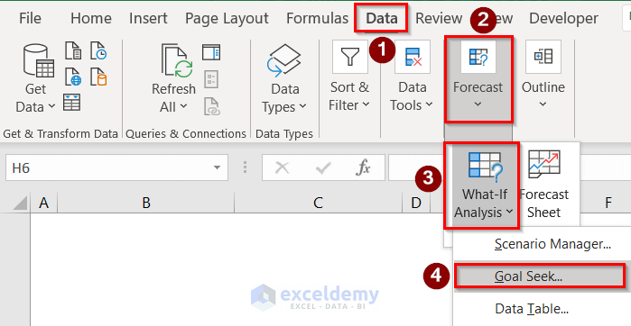
In the Goal Seek dialog box, select cell C17 in the Set cell option (the cell you want to change). Then choose 8000 (the desired value you want to achieve) in the To Value option and select cell C6 (the cell you want to use as the variable) and press OK .

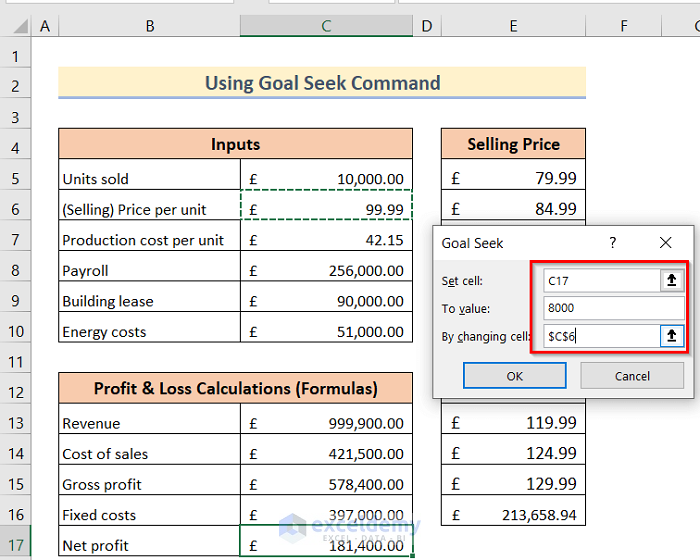
The Goal Seek formula will adjust cell C6 based on the expected value in C17.

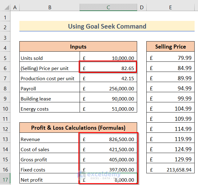
How to Fix “Sensitivity Analysis Not Working in Excel”

Identify if you have a problem like the below image.

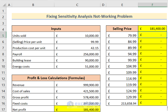
Select the File tab.

Go to More…>Options . The Excel Options dialog box will open on the screen.

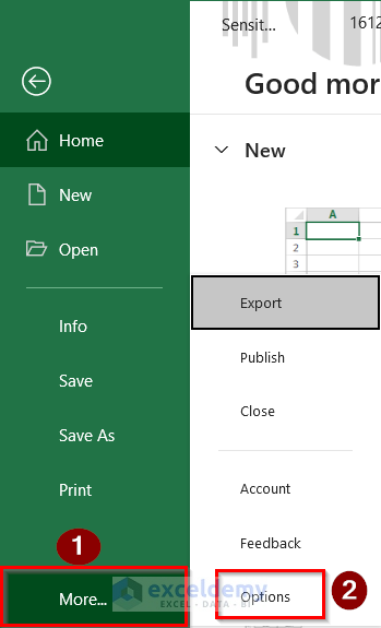
Select the Formulas tab, then choose the Automatic option in the Calculations options and press OK .

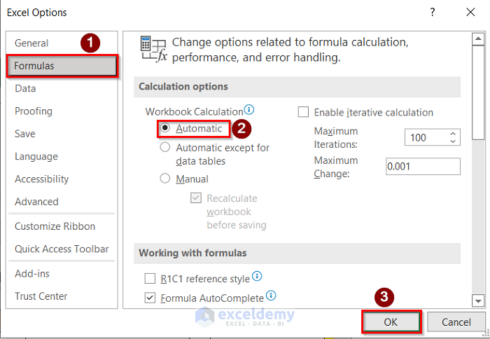
This should fix the table.

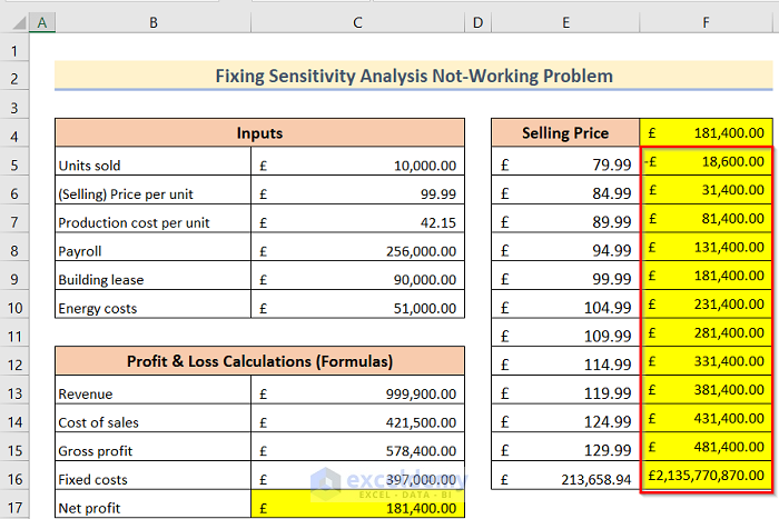
Read More: What If Analysis Data Table Not Working

Download Practice Workbook

You can download the practice workbook from here.

How to Perform Sensitivity Analysis for Capital Budgeting in Excel
How to Get Sensitivity Report from Solver in Excel
Sensitivity Analysis for NPV in Excel
How to Do IRR Sensitivity Analysis in Excel
How to Delete What If Analysis in Excel

<< Go Back to What-If Analysis in Excel | Learn Excel

What is ExcelDemy?

Tags: What if Analysis Excel

Zehad Rian Jim is a dedicated professional with a BSc. Degree in Naval Architecture and Marine Engineering from Bangladesh University of Engineering and Technology. He's good with Microsoft Office and has written more than 80 helpful articles for ExcelDemy in the last year. Now, he makes fun and easy-to-follow Excel tutorials for YouTube as part of the ExcelDemy Video project. Zehad loves figuring out Excel problems, and his passion for learning new things in Excel shines through in... Read Full Bio