Simplex Method for Solution of L.P.P (With Examples) | Operation Research

After reading this article you will learn about:- 1. Introduction to the Simplex Method 2. Principle of Simplex Method 3. Computational Procedure 4. Flow Chart.

Introduction to the Simplex Method :
Simplex method also called simplex technique or simplex algorithm was developed by G.B. Dantzeg, An American mathematician. Simplex method is suitable for solving linear programming problems with a large number of variable. The method through an iterative process progressively approaches and ultimately reaches to the maximum or minimum values of the objective function.
Principle of Simplex Method :
It has not been possible to obtain the graphical solution to the LP problem of more than two variables. For these reasons mathematical iterative procedure known as ‘Simplex Method’ was developed. The simplex method is applicable to any problem that can be formulated in-terms of linear objective function subject to a set of linear constraints.
ADVERTISEMENTS:
The simplex method provides an algorithm which is based on the fundamental theorem of linear programming. This states that “the optimal solution to a linear programming problem if it exists, always occurs at one of the corner points of the feasible solution space.”
The simplex method provides a systematic algorithm which consist of moving from one basic feasible solution to another in a prescribed manner such that the value of the objective function is improved. The procedure of jumping from vertex to the vertex is repeated. The simplex algorithm is an iterative procedure for solving LP problems.
It consists of:
(i) Having a trial basic feasible solution to constraints equation,
(ii) Testing whether it is an optimal solution,
(iii) Improving the first trial solution by repeating the process till an optimal solution is obtained.
Computational Procedure of Simplex Method :
The computational aspect of the simplex procedure is best explained by a simple example.
Consider the linear programming problem:
Maximize z = 3x 1 + 2x 2
Subject to x 1 + x 2 , ≤ 4
x 1 – x 2 , ≤ 2
x 1 , x 2 , ≥ 4
< 2 x v x 2 > 0
The steps in simplex algorithm are as follows:
Formulation of the mathematical model:
(i) Formulate the mathematical model of given LPP.
(ii) If objective function is of minimisation type then convert it into one of maximisation by following relationship
Minimise Z = – Maximise Z*
When Z* = -Z
(iii) Ensure all b i values [all the right side constants of constraints] are positive. If not, it can be changed into positive value on multiplying both side of the constraints by-1.
In this example, all the b i (height side constants) are already positive.
(iv) Next convert the inequality constraints to equation by introducing the non-negative slack or surplus variable. The coefficients of slack or surplus variables are zero in the objective function.
In this example, the inequality constraints being ‘≤’ only slack variables s 1 and s 2 are needed.
Therefore given problem now becomes:

The first row in table indicates the coefficient c j of variables in objective function, which remain same in successive tables. These values represent cost or profit per unit of objective function of each of the variables.
The second row gives major column headings for the simple table. Column C B gives the coefficients of the current basic variables in the objective function. Column x B gives the current values of the corresponding variables in the basic.
Number a ij represent the rate at which resource (i- 1, 2- m) is consumed by each unit of an activity j (j = 1,2 … n).
The values z j represents the amount by which the value of objective function Z would be decreased or increased if one unit of given variable is added to the new solution.
It should be remembered that values of non-basic variables are always zero at each iteration.
So x 1 = x 2 = 0 here, column x B gives the values of basic variables in the first column.
So 5, = 4, s 2 = 2, here; The complete starting feasible solution can be immediately read from table 2 as s 1 = 4, s 2 , x, = 0, x 2 = 0 and the value of the objective function is zero.

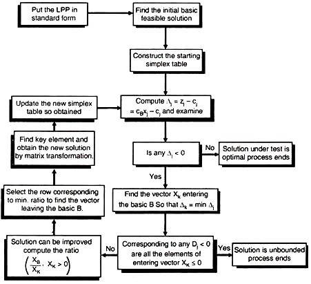
Flow Chart of Simplex Method :
Algorithmic Discussion
There are two theorems in LP:
- The feasible region for an LP problem is a convex set (Every linear equation's second derivative is 0, implying the monotonicity of the trend). Therefore, if an LP has an optimal solution, there must be an extreme point of the feasible region that is optimal
- For an LP optimization problem, there is only one extreme point of the LP's feasible region regarding every basic feasible solution. Plus, there will be a minimum of one basic feasible solution corresponding to every extreme point in the feasible region. [4]

Based on the two theorems above, the geometric illustration of the LP problem could be depicted. Each line of this polyhedral will be the boundary of the LP constraints, in which every vertex will be the extreme points according to the theorem. The simplex method is the way to adjust the nonbasic variables to travel to different vertex till the optimum solution is found. [5]
Consider the following expression as the general linear programming problem standard form:
Failed to parse (SVG (MathML can be enabled via browser plugin): Invalid response ("Math extension cannot connect to Restbase.") from server "https://wikimedia.org/api/rest_v1/":): {\displaystyle \max \sum_{i=1}^n c_ix_i}
With the following constraints:
Failed to parse (SVG (MathML can be enabled via browser plugin): Invalid response ("Math extension cannot connect to Restbase.") from server "https://wikimedia.org/api/rest_v1/":): {\displaystyle \begin{align} s.t. \quad \sum_{j=1}^n a_{ij}x_j &\leq b_i \quad i = 1,2,...,m \\ x_j &\geq 0 \quad j = 1,2,...,n \end{align} }
The first step of the simplex method is to add slack variables and symbols which represent the objective functions:
Failed to parse (SVG (MathML can be enabled via browser plugin): Invalid response ("Math extension cannot connect to Restbase.") from server "https://wikimedia.org/api/rest_v1/":): {\displaystyle \begin{align} \phi &= \sum_{i=1}^n c_ix_i\\ z_i &= b_i - \sum_{j=1}^n a_{ij}x_j \quad i = 1,2,...,m \end{align} }
The new introduced slack variables may be confused with the original values. Therefore, it will be convenient to add those slack variables Failed to parse (SVG (MathML can be enabled via browser plugin): Invalid response ("Math extension cannot connect to Restbase.") from server "https://wikimedia.org/api/rest_v1/":): {\displaystyle z_i } to the end of the list of x -variables with the following expression:
Failed to parse (SVG (MathML can be enabled via browser plugin): Invalid response ("Math extension cannot connect to Restbase.") from server "https://wikimedia.org/api/rest_v1/":): {\displaystyle \begin{align} \phi &= \sum_{i=1}^n c_ix_i\\ x_{n+i} &= b_i - \sum_{j=1}^n a_{ij}x_{ij} \quad i=1,2,...,m \end{align} }
With the progression of simplex method, the starting dictionary (which is the equations above) switches between the dictionaries in seeking for optimal values. Every dictionary will have m basic variables which form the feasible area, as well as n non-basic variables which compose the objective function. Afterward, the dictionary function will be written in the form of:
Where the variables with bar suggest that those corresponding values will change accordingly with the progression of the simplex method. The observation could be made that there will specifically one variable goes from non-basic to basic and another acts oppositely. This kind of variable is referred to as the entering variable . Under the goal of increasing Failed to parse (SVG (MathML can be enabled via browser plugin): Invalid response ("Math extension cannot connect to Restbase.") from server "https://wikimedia.org/api/rest_v1/":): {\displaystyle \phi} , the entering variables are selected from the set {1,2,...,n}. As long as there are no repetitive entering variables can be selected, the optimal values will be found. The decision of which entering variable should be selected at first place should be made based on the consideration that there usually are multiple constraints (n>1). For the Simplex algorithm, the coefficient with the least value is preferred since the major objective is maximization.
The leaving variables are defined as which go from basic to non-basic. The reason of their existence is to ensure the non-negativity of those basic variables. Once the entering variables are determined, the corresponding leaving variables will change accordingly from the equation below:
Failed to parse (SVG (MathML can be enabled via browser plugin): Invalid response ("Math extension cannot connect to Restbase.") from server "https://wikimedia.org/api/rest_v1/":): {\displaystyle x_i = \bar{b_i} - \bar{a_{ik}}x_k \quad i \, \epsilon \, \{ 1,2,...,n+m \}}
Since the non-negativity of entering variables should be ensured, the following inequality can be derived:
Failed to parse (SVG (MathML can be enabled via browser plugin): Invalid response ("Math extension cannot connect to Restbase.") from server "https://wikimedia.org/api/rest_v1/":): {\displaystyle \bar{b_i} - \bar{a_i}x_k \geq 0 \quad i\,\epsilon\, \{1,2,...,n+m \}}
Where Failed to parse (SVG (MathML can be enabled via browser plugin): Invalid response ("Math extension cannot connect to Restbase.") from server "https://wikimedia.org/api/rest_v1/":): {\displaystyle x_k} is immutable. The minimum Failed to parse (SVG (MathML can be enabled via browser plugin): Invalid response ("Math extension cannot connect to Restbase.") from server "https://wikimedia.org/api/rest_v1/":): {\displaystyle x_i} should be zero to get the minimum value since this cannot be negative. Therefore, the following equation should be derived:
Failed to parse (SVG (MathML can be enabled via browser plugin): Invalid response ("Math extension cannot connect to Restbase.") from server "https://wikimedia.org/api/rest_v1/":): {\displaystyle x_k = \frac {\bar{b_i}}{\bar{a_{ik}}} }
Due to the nonnegativity of all variables, the value of Failed to parse (SVG (MathML can be enabled via browser plugin): Invalid response ("Math extension cannot connect to Restbase.") from server "https://wikimedia.org/api/rest_v1/":): {\displaystyle x_k} should be raised to the largest of all of those values calculated from above equation. Hence, the following equation can be derived:
Failed to parse (SVG (MathML can be enabled via browser plugin): Invalid response ("Math extension cannot connect to Restbase.") from server "https://wikimedia.org/api/rest_v1/":): {\displaystyle x_k = \min_{\bar{a_{ik}}>0} \, \frac{\bar{b_i}}{\bar{a_{ik}}} \quad i=1,2,...,n+m}
Once the leaving-basic and entering-nonbasic variables are chosen, reasonable row operation should be conducted to switch from the current dictionary to the new dictionary, as this step is called pivot. [4]
As in the pivot process, the coefficient for the selected pivot element should be one, meaning the reciprocal of this coefficient should be multiplied to every element within this row. Afterward, multiplying this specific row with corresponding coefficients and adding this to different rows, one should get 0 values for all other entries in this pivot element's column.
If there are any negative variables after the pivot process, one should continue finding the pivot element by repeating the process above. At once there are no more negative values for basic and non-basic variables. The optimal solution is found. [6] [7]
Numerical Example
Considering the following numerical example to gain better understanding:
Failed to parse (SVG (MathML can be enabled via browser plugin): Invalid response ("Math extension cannot connect to Restbase.") from server "https://wikimedia.org/api/rest_v1/":): {\displaystyle \max{4x_1+x_2+4x_3}}
with the following constraints:
Failed to parse (SVG (MathML can be enabled via browser plugin): Invalid response ("Math extension cannot connect to Restbase.") from server "https://wikimedia.org/api/rest_v1/":): {\displaystyle \begin{align} 2x_1 + x_2 + x_3 &\leq 2 \\ x_1 + 2x_2 +3x_3 &\leq 4\\ 2x_1 + 2x_2 + x_3 &\leq 8 \\ x_1,x_2,x_3 &\geq 0 \end{align}}
With adding slack variables to get the following equations:
Failed to parse (SVG (MathML can be enabled via browser plugin): Invalid response ("Math extension cannot connect to Restbase.") from server "https://wikimedia.org/api/rest_v1/":): {\displaystyle \begin{align} z - 4x_1 - x_2 -4x_3 &= 0 \\ 2x_1 + x_2 + x_3 + s_1 &= 2 \\ x_1 + 2x_2 + 3x_3 + s_2 &= 4\\ 2x_1 + 2x_2 + x_3 + s_3 &= 8 \\ x_1,x_2,x_3,s_1,s_2,s_3 &\geq 0 \end{align} }
The simplex tableau can be derived as following:
Failed to parse (SVG (MathML can be enabled via browser plugin): Invalid response ("Math extension cannot connect to Restbase.") from server "https://wikimedia.org/api/rest_v1/":): {\displaystyle \begin{array}{c c c c c c c | r} x_1 & x_2 & x_3 & s_1 & s_2 & s_3 & z & b \\ \hline 2 & 1 & 1 & 1 & 0 & 0 & 0 & 2 \\ 1 & 2 & 3 & 0 & 1 & 0 & 0 & 4 \\ 2 & 2 & 1 & 0 & 0 & 1 & 0 & 8 \\ \hline -4 & -1 & -4 & 0 & 0 & 0 & 1 & 0 \end{array} }
In the last row, the column with the smallest value should be selected. Although there are two smallest values, the result will be the same no matter of which one is selected first. For this solution, the first column is selected. After the least coefficient is found, the pivot process will be conducted by searching for the coefficient Failed to parse (SVG (MathML can be enabled via browser plugin): Invalid response ("Math extension cannot connect to Restbase.") from server "https://wikimedia.org/api/rest_v1/":): {\displaystyle \frac{b_i}{x_1} } . Since the coefficient in the first row is 1 and 4 for the second row, the first row should be pivoted. And following tableau can be created:
Failed to parse (SVG (MathML can be enabled via browser plugin): Invalid response ("Math extension cannot connect to Restbase.") from server "https://wikimedia.org/api/rest_v1/":): {\displaystyle \begin{array}{c c c c c c c | r} x_1 & x_2 & x_3 & s_1 & s_2 & s_3 & z & b \\ \hline 1 & 0.5 & 0.5 & 0.5 & 0 & 0 & 0 & 1 \\ 1 & 2 & 3 & 0 & 1 & 0 & 0 & 4 \\ 2 & 2 & 1 & 0 & 0 & 1 & 0 & 8 \\ \hline -4 & -1 & -4 & 0 & 0 & 0 & 1 & 0 \end{array} }
By performing the row operation still every other rows (other than first row) in column 1 are zeroes:
Failed to parse (SVG (MathML can be enabled via browser plugin): Invalid response ("Math extension cannot connect to Restbase.") from server "https://wikimedia.org/api/rest_v1/":): {\displaystyle \begin{array}{c c c c c c c | r} x_1 & x_2 & x_3 & s_1 & s_2 & s_3 & z & b \\ \hline 1 & 0.5 & 0.5 & 0.5 & 0 & 0 & 0 & 1 \\ 0 & 1.5 & 2.5 & -0.5 & 1 & 0 & 0 & 3 \\ 0 & 1 & 0 & -1 & 0 & 1 & 0 & 6 \\ \hline 0 & 1 & -2 & 2 & 0 & 0 & 1 & 4 \end{array} }
Because there is one negative value in last row, the same processes should be performed again. The smallest value in the last row is in the third column. And in the third column, the second row has the smallest coefficients of Failed to parse (SVG (MathML can be enabled via browser plugin): Invalid response ("Math extension cannot connect to Restbase.") from server "https://wikimedia.org/api/rest_v1/":): {\displaystyle \frac{b_i}{x_3}} which is 1.2. Thus, the second row will be selected for pivoting. The simplex tableau is the following:
Failed to parse (SVG (MathML can be enabled via browser plugin): Invalid response ("Math extension cannot connect to Restbase.") from server "https://wikimedia.org/api/rest_v1/":): {\displaystyle \begin{array}{c c c c c c c | r} x_1 & x_2 & x_3 & s_1 & s_2 & s_3 & z & b \\ \hline 1 & 0.5 & 0.5 & 0.5 & 0 & 0 & 0 & 1 \\ 0 & 0.6 & 1 & -0.2 & 0.4 & 0 & 0 & 1.2 \\ 0 & 1 & 0 & -1 & 0 & 1 & 0 & 6 \\ \hline 0 & 1 & -2 & 2 & 0 & 0 & 1 & 4 \end{array} }
By performing the row operation to make other columns 0's, the following could be derived
Failed to parse (SVG (MathML can be enabled via browser plugin): Invalid response ("Math extension cannot connect to Restbase.") from server "https://wikimedia.org/api/rest_v1/":): {\displaystyle \begin{array}{c c c c c c c | r} x_1 & x_2 & x_3 & s_1 & s_2 & s_3 & z & b \\ \hline 1 & 0.2 & 0 & 0.6 & -0.2 & 0 & 0 & 0.4 \\ 0 & 0.6 & 1 & -0.2 & 0.4 & 0 & 0 & 1.2 \\ 0 & -0.1 & 0 & 0.2 & 0.6 & -1 & 0 & -4.2 \\ \hline 0 & 2.2 & 0 & 1.6 & 0.8 & 0 & 1 & 6.4 \end{array} }
There is no need to further conduct calculation since all values in the last row are non-negative. From the tableau above, Failed to parse (SVG (MathML can be enabled via browser plugin): Invalid response ("Math extension cannot connect to Restbase.") from server "https://wikimedia.org/api/rest_v1/":): {\displaystyle x_1} , Failed to parse (SVG (MathML can be enabled via browser plugin): Invalid response ("Math extension cannot connect to Restbase.") from server "https://wikimedia.org/api/rest_v1/":): {\displaystyle x_3} and Failed to parse (SVG (MathML can be enabled via browser plugin): Invalid response ("Math extension cannot connect to Restbase.") from server "https://wikimedia.org/api/rest_v1/":): {\displaystyle z} are basic variables since all rows in their columns are 0's except one row is 1.Therefore, the optimal solution will be Failed to parse (SVG (MathML can be enabled via browser plugin): Invalid response ("Math extension cannot connect to Restbase.") from server "https://wikimedia.org/api/rest_v1/":): {\displaystyle x_1 = 0.4} , Failed to parse (SVG (MathML can be enabled via browser plugin): Invalid response ("Math extension cannot connect to Restbase.") from server "https://wikimedia.org/api/rest_v1/":): {\displaystyle x_2 = 0} , Failed to parse (SVG (MathML can be enabled via browser plugin): Invalid response ("Math extension cannot connect to Restbase.") from server "https://wikimedia.org/api/rest_v1/":): {\displaystyle x_3 = 1.2} , achieving the maximum value: Failed to parse (SVG (MathML can be enabled via browser plugin): Invalid response ("Math extension cannot connect to Restbase.") from server "https://wikimedia.org/api/rest_v1/":): {\displaystyle z = 6.4}
Application
The simplex method can be used in many programming problems since those will be converted to LP (Linear Programming) and solved by the simplex method. Besides the mathematical application, much other industrial planning will use this method to maximize the profits or minimize the resources needed.
Mathematical Problem
The simplex method is commonly used in many programming problems. Due to the heavy load of computation on the non-linear problem, many non-linear programming(NLP) problems cannot be solved effectively. Consequently, many NLP will rely on the LP solver, namely the simplex method, to do some of the work in finding the solution (for instance, the upper or lower bound of the feasible solution), or in many cases, those NLP will be wholly linearized to LP and solved from the simplex method. [1] Other than solving the problems, simplex method can also be used reliably to support the LP's solution from other theorem, for instance the Farkas' theorem in which Simplex method proves the suggested feasible solutions. [1] Besides solving the problems, the Simplex method can also enlighten the scholars with the ways of solving other problems, for instance, Quadratic Programming (QP). [8] For some QP problems, they have linear constraints to the variables which can be solved analogous to the idea of the Simplex method.
Industrial Application
The industries from different fields will use the simplex method to plan under the constraints. With considering that it is usually the case that the constraints or tradeoffs and desired outcomes are linearly related to the controllable variables, many people will develop the models to solve the LP problem via the simplex method, for instance, the agricultural and economic problems
Farmers usually need to rationally allocate the existed resources to obtain the maximum profits. The potential constraints are raised from multiple perspectives including policy restriction, budget concerns as well as farmland area. Farmers may incline to use the simplex-method-based model to have a better plan, as those constraints may be constant in many scenarios and the profits are usually linearly related to the farm production, thereby forming the LP problem. Currently, there is an existing plant-model that can accept inputs such as price, farm production, and return the optimal plan to maximize the profits with given information. [9]
Besides agricultural purposes, the Simplex method can also be used by enterprises to make profits. The rational sale-strategy will be indispensable to the successful practice of marketing. Since there are so many enterprises international wide, the marketing strategy from enamelware is selected for illustration. After widely collecting the data of the quality of varied products manufactured, cost of each and popularity among the customers, the company may need to determine which kind of products well worth the investment and continue making profits as well as which won't. Considering the cost and profit factors are linearly dependent on the production, economists will suggest an LP model that can be solved via the simplex method. [10]
The above professional fields are only the tips of the iceberg to the simplex method application. Many other fields will use this method since the LP problem is gaining popularity in recent days and the simplex method plays a crucial role in solving those problems.
It is indisputable to acknowledge the influence of the Simplex method to programming, as this method won the 'National Medal of Science' to its inventor, George Dantzig. [11] Not only for its wide usage in the mathematic models and industrial manufacture, but the Simplex method also provides a new perspective in solving the inequality problems. As its contribution to the programming substantially boosts the advancement of the current technology and economy from making the optimal plan with the constraints. Nowadays, with the development of technology and economics, the Simplex method is substituted with some more advanced solvers which can solve the problems with faster speed and handle a larger amount of constraints and variables, but this innovative method marks the creativity at that age and continuously offer the inspiration to the upcoming challenges.
- ↑ 1.0 1.1 Linear complementarity, linear and nonlinear programming Internet Edition .
- ↑ Dantzig, G. B. (1987, May). Origins of the simplex method .
- ↑ Strang, G. (1987). Karmarkar’s algorithm and its place in applied mathematics. The Mathematical Intelligencer, 9 (2), 4-10. doi:10.1007/bf03025891.
- ↑ 4.0 4.1 Vanderbei, R. J. (2000). Linear programming: Foundations and extensions . Boston: Kluwer.
- ↑ Sakarovitch M. (1983) Geometric Interpretation of the Simplex Method. In: Thomas J.B. (eds) Linear Programming. Springer Texts in Electrical Engineering. Springer, New York, NY. https://doi.org/10.1007/978-1-4757-4106-3_8
- ↑ Evar D. Nering and Albert W. Tucker, 1993, Linear Programs and Related Problems , Academic Press. (elementary)
- ↑ Robert J. Vanderbei, Linear Programming: Foundations and Extensions , 3rd ed., International Series in Operations Research & Management Science, Vol. 114, Springer Verlag, 2008. ISBN 978-0-387-74387-5.
- ↑ Wolfe, P. (1959). The simplex method for quadratic programming. Econometrica, 27 (3), 382. doi:10.2307/1909468
- ↑ Hua, W. (1998). Application of the revised simplex method to the farm planning model .
- ↑ Nikitenko, A. V. (1996). Economic analysis of the potential use of a simplex method in designing the sales strategy of an enamelware enterprise. Glass and Ceramics, 53 (12), 367-369. doi:10.1007/bf01129674.
- ↑ Cottle, R., Johnson, E. and Wets, R. (2007). George B. Dantzig (1914–2005). Notices Amer. Math. Soc. 54, 344–362.
- Pages with math errors
- Pages with math render errors
Navigation menu

- school Campus Bookshelves
- menu_book Bookshelves
- perm_media Learning Objects
- login Login
- how_to_reg Request Instructor Account
- hub Instructor Commons
Margin Size
- Download Page (PDF)
- Download Full Book (PDF)
- Periodic Table
- Physics Constants
- Scientific Calculator
- Reference & Cite
- Tools expand_more
- Readability
selected template will load here
This action is not available.
4: Linear Programming - The Simplex Method
- Last updated
- Save as PDF
- Page ID 37816

- Rupinder Sekhon and Roberta Bloom
- De Anza College
\( \newcommand{\vecs}[1]{\overset { \scriptstyle \rightharpoonup} {\mathbf{#1}} } \)
\( \newcommand{\vecd}[1]{\overset{-\!-\!\rightharpoonup}{\vphantom{a}\smash {#1}}} \)
\( \newcommand{\id}{\mathrm{id}}\) \( \newcommand{\Span}{\mathrm{span}}\)
( \newcommand{\kernel}{\mathrm{null}\,}\) \( \newcommand{\range}{\mathrm{range}\,}\)
\( \newcommand{\RealPart}{\mathrm{Re}}\) \( \newcommand{\ImaginaryPart}{\mathrm{Im}}\)
\( \newcommand{\Argument}{\mathrm{Arg}}\) \( \newcommand{\norm}[1]{\| #1 \|}\)
\( \newcommand{\inner}[2]{\langle #1, #2 \rangle}\)
\( \newcommand{\Span}{\mathrm{span}}\)
\( \newcommand{\id}{\mathrm{id}}\)
\( \newcommand{\kernel}{\mathrm{null}\,}\)
\( \newcommand{\range}{\mathrm{range}\,}\)
\( \newcommand{\RealPart}{\mathrm{Re}}\)
\( \newcommand{\ImaginaryPart}{\mathrm{Im}}\)
\( \newcommand{\Argument}{\mathrm{Arg}}\)
\( \newcommand{\norm}[1]{\| #1 \|}\)
\( \newcommand{\Span}{\mathrm{span}}\) \( \newcommand{\AA}{\unicode[.8,0]{x212B}}\)
\( \newcommand{\vectorA}[1]{\vec{#1}} % arrow\)
\( \newcommand{\vectorAt}[1]{\vec{\text{#1}}} % arrow\)
\( \newcommand{\vectorB}[1]{\overset { \scriptstyle \rightharpoonup} {\mathbf{#1}} } \)
\( \newcommand{\vectorC}[1]{\textbf{#1}} \)
\( \newcommand{\vectorD}[1]{\overrightarrow{#1}} \)
\( \newcommand{\vectorDt}[1]{\overrightarrow{\text{#1}}} \)
\( \newcommand{\vectE}[1]{\overset{-\!-\!\rightharpoonup}{\vphantom{a}\smash{\mathbf {#1}}}} \)
Learning Objectives
In this chapter, you will:
- Investigate real world applications of linear programming and related methods.
- Solve linear programming maximization problems using the simplex method.
- Solve linear programming minimization problems using the simplex method.
- 4.1: Introduction to Linear Programming Applications in Business, Finance, Medicine, and Social Science In this section, you will learn about real world applications of linear programming and related methods.
- 4.2.1: Maximization By The Simplex Method (Exercises)
- 4.3.1: Minimization By The Simplex Method (Exercises)
- 4.4: Chapter Review
Thumbnail: Polyhedron of simplex algorithm in 3D. (CC BY-SA 3.0; Sdo via Wikipedia)

Chapter 5: Linear Programming with the Simplex Method
One of the most significant advancements in linear programming is the simplex method, developed by George Dantzig. This algorithm provides a systematic approach to finding the optimal solution to linear programming problems. In this article, we will explore the simplex method, its key concepts, and how it is applied to solve linear programming problems.
Overview of the Linear Programming with the Simplex Method
The simplex method is a systematic approach to traverse the vertices of the polyhedron containing feasible solutions in a linear programming problem. It aims to find the optimal solution by iteratively improving the objective function value. This method is considered one of the greatest inventions of modern times due to its broad applicability in solving business-related problems.
Formulating the Original Linear Programming Problem
To illustrate the simplex method, let’s consider a furniture production problem. We want to maximize the revenue generated by producing chairs and tables, subject to constraints on the availability of mahogany and labor. The original problem can be formulated as follows:
- Maximize Revenue = 45×1 + 80×2
- 5×1 + 20×2 ≤ 400 (Mahogany constraint)
- 10×1 + 15×2 ≤ 450 (Labor constraint)
- x1, x2 ≥ 0 (Non-negativity constraint)
In this formulation, x1 represents the number of chairs produced, x2 represents the number of tables produced, and the objective function maximizes the total revenue. The constraints limit the consumption of mahogany and labor within the available capacities.
Transforming into Standard Form
To apply the simplex method, we transform the original problem into the standard form, which involves converting the inequalities into equalities. We introduce slack variables to represent the surplus capacity of each constraint. In this case, we add h1 and h2 as slack variables for the mahogany and labor constraints, respectively. The problem in standard form becomes:
- Maximize Revenue = 45×1 + 80×2 + 0h1 + 0h2
- 5×1 + 20×2 + h1 = 400 (Mahogany constraint)
- 10×1 + 15×2 + h2 = 450 (Labor constraint)
- x1, x2, h1, h2 ≥ 0 (Non-negativity constraint)
The slack variables h1 and h2 represent the unused capacities of mahogany and labor, respectively. We still aim to maximize the revenue while satisfying these transformed equalities.
Basic Feasible Solutions and Canonical Form
A basic feasible solution is an initial production plan that satisfies all the constraints, with some variables set to zero. In our case, the initial solution where no chairs or tables are produced (x1=0, x2=0) represents a basic feasible solution. This solution generates zero revenue, as expected.
The non-basic variables in a basic feasible solution are set to zero, while the basic variables take positive values. In our initial solution, h1 and h2 are the basic variables, representing the unused capacities of mahogany and labor. The non-basic variables are x1 and x2, which are set to zero. This configuration is called a basic feasible solution and is an important concept in linear programming.
To express the problem in canonical form, we represent the basic variables (h1 and h2) in terms of the non-basic variables (x1 and x2). Similarly, we substitute the non-basic variables in the objective function. This process is known as pivoting. The canonical form of the problem becomes:
- Maximize z = 45×1 + 80×2 + 0h1 + 0h2
- x1 = 0 + (1/5)h1 – (4/5)h2 (Transformed mahogany constraint)
- x2 = 0 – (2/5)h1 + (3/5)h2 (Transformed labor constraint)
- x1, x2, h1, h2 ≥ 0
In the canonical form, the objective function and constraints are expressed with respect to the basic variables x1 and x2. The reduced costs associated with the non-basic variables x1 and x2 (coefficients in the objective function) indicate the potential improvement in the objective function value if these variables enter the basis.
Iteration and Optimal Solution
In each iteration of the simplex method, we analyze the non-basic variables and their coefficients. If all the non-basic variables have coefficients ≤ 0, the current solution is optimal. Negative reduced costs associated with the non-basic variables indicate that increasing these variables would decrease the objective function value.
If there is a non-basic variable with a positive reduced cost, we choose the one with the largest coefficient to enter the basis. To determine the maximum value for this variable, we perform the minimum ratio test using the transformed equations. The minimum ratio identifies the constraint that limits the increase of the non-basic variable while staying feasible.
After selecting the entering variable, we perform pivoting to express the problem in canonical form with respect to the new basic variables. This process continues iteratively until we reach an optimal solution or determine that the problem is unbounded.
The simplex method provides a systematic approach to solving linear programming problems by iteratively improving the objective function value. By transforming the problem into the standard form and expressing it in canonical form, we can identify basic feasible solutions and optimize the objective function. The simplex method is a fundamental tool in linear programming, enabling efficient optimization in various industries and applications.
Download the complete Linear Programming Tutorial Series slide deck .
View the entire series:
- Welcome: Linear Programming Tutorial
- Chapter 1: Mathematical Programming
- Chapter 2: Introduction to Linear Programming
- Chapter 3: Mixed Integer Linear Programming Problems
- Chapter 4: Furniture Factory Problem
- Chapter 5: Simplex Method
- Chapter 6: Modeling and Solving Linear Programming Problems
- Chapter 7: Sensitivity Analysis of Linear Programming Problems
- Chapter 8: Multiple Optimal Solutions
- Chapter 9: Unbounded Linear Programming Problems
- Chapter 10: Infeasible Linear Programming Problems
- Chapter 11: Linear Programming Overview – Further Considerations
- Chapter 12: Duality in Linear Programming
- Chapter 13: Optimality Conditions
- Chapter 14: Dual Simplex Method
Guidance for Your Journey
30 day free trial for commercial users, always free for academics.
GUROBI NEWSLETTER
Latest news and releases
- The role of crossover in linear programming
- Linear Programming (LP) – A Primer on the Basics
Try Gurobi for Free
Choose the evaluation license that fits you best, and start working with our Expert Team for technical guidance and support.
Evaluation License
Academic license, cloud trial.
Request free trial hours, so you can see how quickly and easily a model can be solved on the cloud.
Looking for documentation?
Jupyter Models
Case studies, privacy overview.
- Math Article
- Linear Programming Problem Lpp
Linear programming problem (LPP)

Linear Programming Problems (LPP): Linear programming or linear optimization is a process which takes into consideration certain linear relationships to obtain the best possible solution to a mathematical model. It is also denoted as LPP. It includes problems dealing with maximizing profits, minimizing costs, minimal usage of resources, etc. These problems can be solved through the simplex method or graphical method.
The Linear programming applications are present in broad disciplines such as commerce, industry, etc. In this section, we will discuss, how to do the mathematical formulation of the LPP.
Mathematical Formulation of Problem
Let x and y be the number of cabinets of types 1 and 2 respectively that he must manufacture. They are non-negative and known as non-negative constraints.
The company can invest a total of 540 hours of the labour force and is required to create up to 50 cabinets. Hence,
15x + 9y <= 540
x + y <= 50
The above two equations are known as linear constraints.
Let Z be the profit he earns from manufacturing x and y pieces of the cabinets of types 1 and 2. Thus,
Z = 5000x + 3000y
Our objective here is to maximize Z. Hence Z is known as the objective function. To find the answer to this question, we use graphs, which is known as the graphical method of solving LPP. We will cover this in the subsequent sections.
Graphical Method
The solution for problems based on linear programming is determined with the help of the feasible region, in case of graphical method. The feasible region is basically the common region determined by all constraints including non-negative constraints, say, x,y≥0, of an LPP. Each point in this feasible region represents the feasible solution of the constraints and therefore, is called the solution/feasible region for the problem. The region apart from (outside) the feasible region is called as the infeasible region .
The optimal value (maximum and minimum) obtained of an objective function in the feasible region at any point is called an optimal solution. To learn the graphical method to solve linear programming completely reach us.
Linear Programming Applications
Let us take a real-life problem to understand linear programming. A home décor company received an order to manufacture cabinets. The first consignment requires up to 50 cabinets. There are two types of cabinets. The first type requires 15 hours of the labour force (per piece) to be constructed and gives a profit of Rs 5000 per piece to the company. Whereas, the second type requires 9 hours of the labour force and makes a profit of Rs 3000 per piece. However, the company has only 540 hours of workforce available for the manufacture of the cabinets. With this information given, you are required to find a deal which gives the maximum profit to the décor company.

Given the situation, let us take up different scenarios to analyse how the profit can be maximized.
- He decides to construct all the cabinets of the first type. In this case, he can create 540/15 = 36 cabinets. This would give him a profit of Rs 5000 × 36 = Rs 180,000.
- He decides to construct all the cabinets of the second type. In this case, he can create 540/9 = 60 cabinets. But the first consignment requires only up to 50 cabinets. Hence, he can make profit of Rs 3000 × 50 = Rs 150,000.
- He decides to make 15 cabinets of type 1 and 35 of type 2. In this case, his profit is (5000 × 15 + 3000 × 35) Rs 180,000.
Similarly, there can be many strategies which he can devise to maximize his profit by allocating the different amount of labour force to the two types of cabinets. We do a mathematical formulation of the discussed LPP to find out the strategy which would lead to maximum profit.
Related Links
To learn more about solving LPP, download BYJU’S The Learning App.
Leave a Comment Cancel reply
Your Mobile number and Email id will not be published. Required fields are marked *
Request OTP on Voice Call
Post My Comment
Register with BYJU'S & Download Free PDFs
Register with byju's & watch live videos.
Help | Advanced Search
Computer Science > Machine Learning
Title: pdhg-unrolled learning-to-optimize method for large-scale linear programming.
Abstract: Solving large-scale linear programming (LP) problems is an important task in various areas such as communication networks, power systems, finance and logistics. Recently, two distinct approaches have emerged to expedite LP solving: (i) First-order methods (FOMs); (ii) Learning to optimize (L2O). In this work, we propose an FOM-unrolled neural network (NN) called PDHG-Net, and propose a two-stage L2O method to solve large-scale LP problems. The new architecture PDHG-Net is designed by unrolling the recently emerged PDHG method into a neural network, combined with channel-expansion techniques borrowed from graph neural networks. We prove that the proposed PDHG-Net can recover PDHG algorithm, thus can approximate optimal solutions of LP instances with a polynomial number of neurons. We propose a two-stage inference approach: first use PDHG-Net to generate an approximate solution, and then apply PDHG algorithm to further improve the solution. Experiments show that our approach can significantly accelerate LP solving, achieving up to a 3$\times$ speedup compared to FOMs for large-scale LP problems.
Submission history
Access paper:.
- HTML (experimental)
- Other Formats
References & Citations
- Google Scholar
- Semantic Scholar
BibTeX formatted citation
Bibliographic and Citation Tools
Code, data and media associated with this article, recommenders and search tools.
- Institution
arXivLabs: experimental projects with community collaborators
arXivLabs is a framework that allows collaborators to develop and share new arXiv features directly on our website.
Both individuals and organizations that work with arXivLabs have embraced and accepted our values of openness, community, excellence, and user data privacy. arXiv is committed to these values and only works with partners that adhere to them.
Have an idea for a project that will add value for arXiv's community? Learn more about arXivLabs .
IMAGES
VIDEO
COMMENTS
The simplex method begins at a corner point where all the main variables, the variables that have symbols such as x1 x 1, x2 x 2, x3 x 3 etc., are zero. It then moves from a corner point to the adjacent corner point always increasing the value of the objective function. In the case of the objective function Z = 40x1 + 30x2 Z = 40 x 1 + 30 x 2 ...
Learn how to solve linear programming problems using the simplex method, a mathematical iterative procedure that improves the value of the objective function. See the steps, rules, and a detailed example with a table and a flow chart.
Linear Programming: Chapter 2 The Simplex Method Robert J. Vanderbei October 17, 2007 ... This is how we detect unboundedness with the simplex method. Initialization Consider the following problem: maximize 3x 1 + 4x 2 subject to 4x 1 2x 2 8 2x 1 2 3x 1 + 2x 2 10 x 1 + 3x 2 1 3x 2 2 x 1;x
2. The simplex method (with equations) The problem of the previous section can be summarized as follows. Maximize the function xˆ = 5x 1 +4x2 subject to the constraints: x 1 +3x2 18 x 1 + x2 8 2x 1 + x2 14 where we also assume that x 1, x2 0. Linear algebra provides powerful tools for simplifying linear equations. The first step
invented the simplex method to efficiently find the optimal solution for linear programming problems. The simplex method is an alternate method to graphing that can be used to solve linear programming problems—particularly those with more than two variables. We first list the algorithm for the simplex method, and then we examine a few ...
The Simplex Method: Solving Standard Maximization Problems / Método simplex.
Simplex Method: Example 1. Maximize z = 3x 1 + 2x 2. subject to. -x 1 + 2x 2 ≤ 4. 3x 1 + 2x 2 ≤ 14. x 1 - x 2 ≤ 3. x 1, x 2 ≥ 0. Solution. First, convert every inequality constraints in the LPP into an equality constraint, so that the problem can be written in a standard from.
Simplex algorithm (or Simplex method) is a widely-used algorithm to solve the Linear Programming (LP) optimization problems. The simplex algorithm can be thought of as one of the elementary steps for solving the inequality problem, since many of those will be converted to LP and solved via Simplex algorithm. [1]
I Optimization problem (Simplex method) Examples and standard form Fundamental theorem Simplex algorithm Linear programming I Definition: If the minimized (or maximized) function and the constraints are all in ... Solving x 1 from one equation and substitute it into others. x 1 = 5 − 2x 2 − x 3 then minw = 5 + x 2 + 3x 3 s.t. x
Solving Linear Programming Problems: The Simplex Method We now are ready to begin studying the simplex method,a general procedure for solving linear programming problems. Developed by George Dantzig in 1947, it has proved to be a remarkably efficient method that is used routinely to solve huge problems on today's computers.
In this video detail explanation is given for each steps of simplex method to solve maximization type LPP. Also comparison of graphical method and simplex me...
In this video we can learn Linear Programming problem using Simplex Method using a simple logic with solved problem, hope you will get knowledge in it. NOTE:...
Learning Objectives. In this chapter, you will: Investigate real world applications of linear programming and related methods. Solve linear programming maximization problems using the simplex method. Solve linear programming minimization problems using the simplex method. Thumbnail: Polyhedron of simplex algorithm in 3D.
In this article, we will explore the simplex method, its key concepts, and how it is applied to solve linear programming problems. Overview of the Linear Programming with the Simplex Method. The simplex method is a systematic approach to traverse the vertices of the polyhedron containing feasible solutions in a linear programming problem.
The simplex method. Two important characteristics of the simplex method: The method is robust. It solves any linear program; It detects redundant constraints in the problem formulation; It identifies instances when the objective value is unbounded over the feasible region; and. It solves problems with one or more optimal solutions.
Learn how to solve linear programming problems (LPP) using simplex and graphical methods with examples and applications. Find out the optimal solution, feasible region, objective function and constraints of LPP.
Here is the video about LPP using simplex method (Minimization) with three variables, in that we have discussed that how to solve the simplex method minimiza...
Simplex Method of Linear Programming Marcel Oliver Revised: September 28, 2020 1 The basic steps of the simplex algorithm Step 1: Write the linear programming problem in standard form Linear programming (the name is historical, a more descriptive term would be linear optimization) refers to the problem of optimizing a linear objective
simplex method, standard technique in linear programming for solving an optimization problem, typically one involving a function and several constraints expressed as inequalities. The inequalities define a polygonal region, and the solution is typically at one of the vertices. The simplex method is a systematic procedure for testing the vertices as possible solutions.
4.8 Dual Linear Programming Problem 4.9 Summary 4.10 Key Words 4.11 Self-assessment Exercises 4.12 Answers 4.13 Further Readings 4.1 INTRODUCTION Although the graphical method of solving linear programming problem is an invaluable aid to understand its basic structure, the method is of limited application in
After utilizing mean and median techniques, the problem is converted into an equivalent linear fractional programming problem; then, the linear fractional programming problem is transformed into linear programming problem and solved by the conventional simplex method or mathematical software.
Recently, two distinct ap-proaches have emerged to expedite LP solving: (i) First-order methods (FOMs); (ii) Learning to optimize (L2O). In this work, we propose a FOM-unrolled neural network (NN) called PDHG-Net, and propose a two-stage L2O method to solve large-scale LP problems. The new architecture PDHG-Net is designed by unrolling the ...
Solving large-scale linear programming (LP) problems is an important task in various areas such as communication networks, power systems, finance and logistics. Recently, two distinct approaches have emerged to expedite LP solving: (i) First-order methods (FOMs); (ii) Learning to optimize (L2O). In this work, we propose an FOM-unrolled neural network (NN) called PDHG-Net, and propose a two ...