solve xor problem in neural network

• Conferences
• Last updated June 29, 2022
• In AI Mysteries

XOR problem with neural networks: An explanation for beginners

• Published on June 29, 2022
• by Darshan M

Among various logical gates, the XOR or also known as the “exclusive or” problem is one of the logical operations when performed on binary inputs that yield output for different combinations of input, and for the same combination of input no output is produced. The outputs generated by the XOR logic are not linearly separable in the hyperplane. So  In this article let us see what is the XOR logic and how to integrate the XOR logic using neural networks.

Table of Contents

What is xor operating logic, the linear separability of points, why can’t perceptrons solve the xor problem, how to solve the xor problem with neural networks.

Let us try to understand the XOR operating logic using a truth table.

From the below truth table it can be inferred that XOR produces an output for different states of inputs and for the same inputs the XOR logic does not produce any output. The Output of XOR logic is yielded by the equation as shown below.

Output= X.Y’+X’.Y

The XOR gate can be usually termed as a combination of NOT and AND gates and this type of logic finds its vast application in cryptography and fault tolerance. The logical diagram of an XOR gate is shown below.

Are you looking for a complete repository of Python libraries used in data science,  check out here .

Linear separability of points is the ability to classify the data points in the hyperplane by avoiding the overlapping of the classes in the planes. Each of the classes should fall above or below the separating line and then they are termed as linearly separable data points. With respect to logical gates operations like AND or OR the outputs generated by this logic are linearly separable in the hyperplane

The linear separable data points appear to be as shown below.

So here we can see that the pink dots and red triangle points in the plot do not overlap each other and the linear line is easily separating the two classes where the upper boundary of the plot can be considered as one classification and the below region can be considered as the other region of classification.

Need for linear separability in neural networks

Linear separability is required in neural networks is required as basic operations of neural networks would be in N-dimensional space and the data points of the neural networks have to be linearly separable to eradicate the issues with wrong weight updation and wrong classifications Linear separability of data is also considered as one of the prerequisites which help in the easy interpretation of input spaces into points whether the network is positive and negative and linearly separate the data points in the hyperplane.

Perceptrons are mainly termed as “linear classifiers” and can be used only for linear separable use cases and XOR is one of the logical operations which are not linearly separable as the data points will overlap the data points of the linear line or different classes occur on a single side of the linear line. 

Let us understand why perceptrons cannot be used for XOR logic using the outputs generated by the XOR logic and the corresponding graph for XOR logic as shown below.

In the above figure, we can see that above the linear separable line the red triangle is overlapping with the pink dot and linear separability of data points is not possible using the XOR logic. So this is where multiple neurons also termed as Multi-Layer Perceptron are used with a hidden layer to induce some bias while weight updation and yield linear separability of data points using the XOR logic. So now let us understand how to solve the XOR problem with neural networks.

The XOR problem with neural networks can be solved by using Multi-Layer Perceptrons or a neural network architecture with an input layer, hidden layer, and output layer. So during the forward propagation through the neural networks, the weights get updated to the corresponding layers and the XOR logic gets executed. The Neural network architecture to solve the XOR problem will be as shown below.

So with this overall architecture and certain weight parameters between each layer, the XOR logic output can be yielded through forward propagation. The overall neural network architecture uses the Relu activation function to ensure the weights updated in each of the processes to be 1 or 0 accordingly where for the positive set of weights the output at the particular neuron will be 1 and for a negative weight updation at the particular neuron will be 0 respectively. So let us understand one output for the first input state 

Example :  For X1=0 and X2=0 we should get an input of 0. Let us solve it.

Solution: Considering X1=0 and X2=0

H1=RELU(0.1+0.1+0) = 0

H2=RELU(0.1+0.1+0)=0

So now we have obtained the weights that were propagated from the input layer to the hidden layer. So now let us propagate from the hidden layer to the output layer

Y=RELU(0.1+0.(-2))=0

This is how multi-layer neural networks or also known as Multi-Layer perceptrons (MLP) are used to solve the XOR problem and for all other input sets the architecture provided above can be verified and the right outcome for XOR logic can be yielded.

So among the various logical operations, XOR logical operation is one such problem wherein linear separability of data points is not possible using single neurons or perceptrons. So for solving the XOR problem for neural networks it is necessary to use multiple neurons in the neural network architecture with certain weights and appropriate activation functions to solve the XOR problem with neural networks.

Access all our open Survey & Awards Nomination forms in one place

Can LNNs Replace Transformers?

Stop Confusing Calculators with GPT-4

Google introduces ktn to solve label scarcity in heterogeneous graphs, chatgpt privacy threat is real and we are late.

Going Beyond Large Language Models (LLMs)

Think Like Yoshua

Do AI Models Really Understand The Human Brain?

Is Reinforcement Learning Still Relevant?

The announcement comes right after OpenAI disbanded its super alignment team led by Ilya Sutskever and Jan Leike.

Top Editorial Picks

Google is Giving Away a Custom Electric 1981 DeLorean as Grand Prize in ‘Gemini API Developer Competition’ Siddharth Jindal

Bhashini Launches ‘Be our Sahayogi’ for Multilingual AI Innovation Focused on Voice Mohit Pandey

Jivi’s Medical LLM Beats OpenAI at the Open Medical LLM Leaderboard Pritam Bordoloi

CtrlS Launches 13-MW, AI-ready Data Center in Hyderabad Shyam Nandan Upadhyay

Agnikul Cosmos Launches India’s Second Private Rocket, Agnibaan SOrTeD Shyam Nandan Upadhyay

UiPath Stock Plunges Nearly 30% as CEO Rob Enslin Abruptly Resigns Shyam Nandan Upadhyay

Meta Introduces Vision Language Models, Shows Superior Performance Over Traditional CNNs Sukriti Gupta

Subscribe to The Belamy: Our Weekly Newsletter

Biggest ai stories, delivered to your inbox every week., "> "> flagship events.

Explore the transformative journey of Global Capability Centers at MachineCon GCC Summit 2024, where innovation meets strategic growth.

© Analytics India Magazine Pvt Ltd & AIM Media House LLC 2024

• Terms of use
• Privacy Policy

Subscribe to Our Newsletter

The Belamy, our weekly Newsletter is a rage. Just enter your email below.

There must be a reason why +150K people have chosen to follow us on LinkedIn. 😉

Stay in the know with our linkedin page. follow us and never miss an update on ai.

• Master Data Science
• Generative Adversarial Networks (GANs)
• Linear Algebra
• Shallow Neural Networks
• Deep Learning
• Master TensorFlow 2.0
• Camera Calibration and Stereo Vision
• OpenCV for Hackers
• Master PyTorch
• Advanced Computer Vision
• Machine Learning
• OpenCV projects
• 7Hours sprint to Data Science
• Computer Vision OpenCV Book
• Popular News

#006 PyTorch – Solving the famous XOR problem using Linear classifiers with PyTorch

Highlights : One of the most historical problems in the Neural Network arena is the classic XOR problem where predicting the output of the ‘Exclusive OR’ gate becomes increasingly difficult using traditional linear classifier methods.

In this post, we will study the expressiveness and limitations of Linear Classifiers, and understand how to solve the XOR problem in two different ways. So let’s begin.

Tutorial Overview:

• Logistic Regression Model

The OR Problem

The and problem, the nand problem.

• Historical Research on XOR

Linear Classifier with Non-Linear Features

• The XOR Problem: Formal Solution

Solving the AND problem

Solving the or problem, solving the nand problem, solving the xor problem, creating the third dimension.

This post is inspired by the following YouTube video [ 1 ]

1. Logistic Regression Model

Let’s start by refreshing our memory with the basic mathematical representation of the Logistic Regression Model as seen below.

$$ \hat{y}=\sigma\left(\mathbf{w}^{\top} \mathbf{x}\right) $$

$$ \sigma(z)=\frac{1}{1+e^{-z}} $$

The above expression shows that in the Linear Regression Model, we have a linear or affine transformation between an input vector \(x \) and a weight vector \(w \). The input vector \(x \) is then turned to scalar value and passed into a non-linear sigmoid function. This sigmoid function compresses the whole infinite range into a more comprehensible range between 0 and 1.

Using the output values between this range of 0 and 1, we can determine whether the input \(x\) belongs to Class 1 or Class 0.

Let’s understand this better using an example of 2D Logistic Regression.

Example: 2D Logistic Regression

For better understanding, let us assume that all our input values are in the 2-dimensional domain. Observe the expression below, where we have a vector \(x\) that contains two elements, \(x_1\) and \(x_2\) respectively.

$$ \hat{y}=\sigma\left(\mathbf{w}^{\top} \mathbf{x}+w_{0}\right) $$

$$ \text { Let } \mathbf{x} \in \mathbb{R}^{2} $$

For each of the element of the input vector \(x\), i.e., \(x_1\) and \(x_2\), we will multiply a weight vector \(w\) and a bias \(w_0\). We, then, convert the vector \(x\) into a scalar value represented by \(z\) and passed onto the sigmoid function. 

Let us represent this example using a graph.

Notice how the Decision Boundary line for this example is exactly at 0. This is due to the fact that when \(z = 0 \), the sigmoid function changes from being below 0.5 to being above 0.5. In simpler words, the probability of the input belonging to Class 1 is higher on the right-hand side of the Decision Boundary line. And, the probability of the input belonging to Class 0 is higher on the left-hand side of the Decision Boundary line. The equation for this Decision Boundary line is written as follows.

$$ \mathbf{w}^{\top} \mathbf{x}+w_{0}=0 $$

To better visualize the above classification, let’s see the graph below.

A total of three scenarios arise as we can see above.

• If \(z<0\), where \(z= w^Tx+w_0\), we decide for Class 0
• If \(z=0\), where \(z= w^Tx+w_0\), we are at the Decision Boundary and uncertain of the Class
• If \(z>0\), where \(z= w^Tx+w_0\), we decide for Class 1

Now that we have a fair recall of the logistic regression models, let us use some linear classifiers to solve some simpler problems before moving onto the more complex XOR problem.

2. Simple Logical Boolean Operator Problems

Before we head over to understanding the problems associated with predicting the XOR operator, let us see how simple linear classifiers can be used to solve lesser complex Boolean operators.

As seen above, the classification rule from our 2D logistic regression model is written as follows.

$$ \text { Class } 1 \Leftrightarrow \mathbf{w}^{\top} \mathbf{x}>-w_{0} $$

Now, in order to implement our classifier as seen above, we need to determine our two important parameters, the weight \(w\) and the bias \(w_0\) such that our decision boundary line clearly separates Class 1 (red) and Class 0 (green). Intuitively, it is not difficult to imagine a line that will separate the two classes.

So, we have successfully classified the OR operator. Let’s see how we can perform the same procedure for the AND operator.

Again, our main task is to determine the optimal parameters, the weight \(w\) and the bias \(w_0\) to draw a decision boundary line separating the two classes. Using trial and error, and some intuition of course, we come to a conclusion that our parameter values should be \(w = (1,1)\) and \(w_0 = -1.5\) respectively. Let’s see how our decision boundary line appears on the graph.

Great! Let’s look at NAND operation, next.

The values for our parameters that we can arrive at here are \(w = (-1,-1)\) and \(w_0 = 1.5\) such that the decision boundary line looks something like this.

As we saw above, simple linear classifiers can easily solve the basic Boolean operator problems. However, when it comes to the XOR operator, things start to become a little complex. Let’s move on to the classic XOR problem.

3. The XOR Problem: Intuitive Solution

Observe the points on the graph above. Our intuition fails to recognize a way to draw a decision boundary line that will clearly separate the two classes.

Similarly, if we were to use the decision boundary line for the NAND operator here, it will also classify 2 out of 3 points correctly.

It is evident that the XOR problem CAN NOT be solved linearly . This is the reason why this XOR problem has been a topic of interest among researchers for a long time.

However, more than just intuitively, we should also prove this theory more formally. We will take the help of Convex Sets to be able to prove that the XOR operator is not linearly separable. Let’s see how.

Convex Sets

Let’s consider a set \(S\).

The set \(S\) is said to be ‘convex’ if any line segment that joins two points within this set \(S\) lies entirely within the set \(S\). We can represent a convex set mathematically as follows:

$$ \mathbf{x}_{1}, \mathbf{x}_{2} \in \mathcal{S} \Rightarrow \lambda \mathbf{x}_{1}+(1-\lambda) \mathbf{x}_{2} \in \mathcal{S} $$

$$ \text { for } \quad \lambda \in[0,1] $$

The image on the left cannot be considered to be a convex set as some of the points on the line joining two points from \(S\) lie outside of the set \(S\). On the right-hand side, however, we can see a convex set where the line segment joining the two points from \(S\) lies completely inside the set \(S\).

Now, convex sets can be used to better visualize our decision boundary line, which divides the graph into two halves that extend infinitely in the opposite directions. We can intuitively say that these half-spaces are nothing but convex sets such that no two points within these half-spaces lie outside of these half-spaces.

This is clearly a wrong hypothesis and doesn’t hold valid simply because the intersection point of the green and the red line segment cannot lie in both the half-spaces. This means that the intersection point of the two lines cannot be classified in both Class 0 as well as Class 1. Therefore, we have arrived at a contradiction .

This provides formal proof of the fact that the XOR operators cannot be solved linearly.

Historical Research On XOR

In the 1950s and the 1960s, linear classification was widely used and in fact, showed significantly good results on simple image classification problems such as the Perceptron.

Perceptron – an electronic device that was constructed in accordance with biological principles and showed an ability to learn [2]

However, with the 1969 book named ‘Perceptrons’, written by Minsky and Paper, the limitations of using linear classification became more apparent. It became evident that even a problem like the XOR operator, which looks simple on the face of it with just 4 data points, cannot be solved easily since the classifier models available to us at that time were only capable of making linear decisions.

Naturally, due to rising limitations, the use of linear classifiers started to decline in the 1970s and more research time was being devoted to solving non-linear problems.

Moving ahead, let’s study a Linear Classifier with non-linear features and see if it can help us in solving our XOR problem.

In this case, we will consider an extended feature space such as the following:

$$ \mathbf{w}^{\top} \underbrace{\left(\begin{array}{c}x_{1} \\x_{2} \\x_{1} x_{2}\end{array}\right)}_{\psi(\mathbf{x})}>-w_{0} $$

Observe how the green points are below the plane and the red points are above the plane. This plane is nothing but the XOR operator’s decision boundary.

So, by shifting our focus from a 2-dimensional visualization to a 3-dimensional one, we are able to classify the points generated by the XOR operator far more easily.

This exercise brings to light the importance of representing a problem correctly. If we represent the problem at hand in a more suitable way, many difficult scenarios become easy to solve as we saw in the case of the XOR problem. Let’s understand this better.

Representational Learning

Notice the left-hand side image which is based on the Cartesian coordinates. There is no intuitive way to distinguish or separate the green and the blue points from each other such that they can be classified into respective classes.

However, when we transform the dataset to Polar coordinates, i.e., represent them in terms of radius and angle, we can notice how it becomes intuitively possible to draw a linear decision boundary line that classifies each point separately.

Representing data to help you make better decisions while creating your models is what Deep Learning is all about. But, how does one choose the right transformation?

Until the 2000s, choosing the transformation was done manually for problems such as vision, speech, etc. using histogram of gradients to study regions of interest. Having said that, today, we can safely say that rather than doing this manually, it is always better to have your model or computer learn, train, and decide which transformation to use automatically. This is what Representational Learning is all about, wherein, instead of providing the exact function to our model, we provide a family of functions for the model to choose the appropriate function itself.

Now that we have seen how we can solve the XOR problem using an observational, representational, and intuitive approach, let’s look at the formal solution for the XOR problem.

4. The XOR Problem: Formal Solution

One solution for the XOR problem is by extending the feature space and using a more non-linear feature approach. This can be termed as more of an intuitive solution. However, we must understand how we can solve the XOR problem using the traditional linear approach as well.

By combining the two decision boundaries of OR operator and NAND operator respectively using an AND operation, we can obtain the exact XOR classifier.

We can write this mathematically as follows:

$$ \begin{array}{c}\text { XOR }\left(x_{1}, x_{2}\right)= \\\text { AND(OR }\left(x_{1}, x_{2}\right), \text { NAND } \left.\left(x_{1}, x_{2}\right)\right)\end{array} $$

Now, the above expression can be rewritten as a program of multiple logistic regressions. Have a look.

$$ h_{1}=\sigma\left(\mathbf{w}_{O R}^{\top} \mathbf{x}+w_{O R}\right) $$

$$ h_{2}=\sigma\left(\mathbf{w}_{N A N D}^{\prime} \mathbf{x}+w_{N A N D}\right) $$

$$ \hat{y}=\sigma\left(\mathbf{w}_{A N D}^{\top} \mathbf{h}+w_{A N D}\right) $$

This multi-later ‘perceptron’ has two hidden layers represented by \(h_1\) and \(h_2\), where \(h(x)\) is a non-linear feature of \(x\). We can represent this network visually as follows.

We can, further, simplify the above 1D mappings as a single 2D mapping as follows.

$$ \mathbf{h}=\sigma\underbrace{\left(\begin{array}{c}\mathbf{w}_{O R}^{\top}\\\left.\mathbf{w}_{NAND}^{\top}\right)\end{array}\right)}_{\mathbf{W}}\mathbf{x}+\underbrace{\left(\begin{array}{c}w_{OR}\\w_{NAND}\end{array}\right)}_{\mathbf{w}} $$

The biggest advantage of using the above solution for the XOR problem is that now, we don’t have non-differentiable step-functions anymore. Instead, we have differential equations sigmoid activation functions which means we can start with a random guess for each of the parameters in our model and later, optimize according to our dataset. This parametric learning is done using gradient descent where the gradients are calculated using the back-propagation algorithm.

Let’s now see how we can solve the XOR problem in Python using PyTorch.

5. Solving The XOR Problem in Python using PyTorch

Let’s start by importing the necessary libraries.

First, we’ll create the data for the logical operator AND. First, we will create our decision table were x1 and x2 are two NumPy arrays consisting of four numbers. These arrays will represent the binary input for the AND operator. Then, we will create an output array y , and we will set the data type to be equal to np.float32 . 

Now, we can scatter our data points. Here, x1 and x2 will be the coordinates of the points and color will depend on y . Let’s have a look at the following graph. 

We can see that just the yellow point will have a value of 1, while the remaining three points will have a value of 0. 

The next step would be to create a data set because we cannot just train our data on these four points. So, we will create a function create_dataset() that will accept x1 , x2 and y as our input parameters. Then, we will use the function np. repeat() to repeat every number in x1 , x2 , and y 50 times. In that way, we will have 200 numbers in each array.

After this, we also need to add some noise to x1 and x2 arrays. We can do that by using the np.random.rand() function and pass width of an array multiplied with some small number (in our case it is 0.05). 

The next step is to shuffle the data. We will create an index_shuffle variable and apply np.arrange() function on x1.shape[0] . This function will return 200 numbers from zero to 200. Next, we will use the function  np.random.shuffle() on the variable index_shuffle . 

After we set the data type to be equal to np.float32 ,  we can apply this index shuffle variable on x1 , x2 and y . 

Now, remember, because we are using PyTorch we need to convert our data to tensors. Once we do that we will combine x1 and x2 .  We will create a variable X and apply the function torch.hstack() to stack horizontally x1_torch and x2_torch tensors.  

The next step is to create a training and testing data set for X and y . So, we will create X_train , X_test , y_train and y_test . Then for the X_train and y_tarin, we will take the first 150 numbers, and then for the X_test and y_test, we will take the last 150 numbers.  Finally, we will return X_train, X_test, y_train, and y_test.

Now we can call the function create_dataset() and plot our data.

The next step is to create the LogisticRegression() class. To be able to use it as a PyTorch model, we will pass torch. nn.Module as a parameter. Then, we will define the init() function by passing the parameter self .

Now that we have created the class for the Logistic regression, we need to create the model for AND logical operator. So, we will create the variable model_AND which will be equal to LogisticRegression() class. As parameters we will pass number 2 and 1 because our  x now has two features, and we want one output for the y . Then, we will create a criterion where we will calculate the loss using the function torch.nn.BCELoss() ( Binary Cross Entropy Loss). Also we need to define an optimizer by using the Stochastic Gradient descent. As parameters we will pass model_AND.parameters() , and we will set the learning rate to be equal to 0.01 . 

Now that we have defined everything we need, we’ll create a training function. As an input, we will pass model , criterion , optimizer , X , y and a number of iterations. Then, we will create a list where we will store the loss for each epoch. We will create a for loop that will iterate for each epoch in the range of iteration. 

The next step is to apply the forward propagation. We will define prediction y_hat and we will calculate the loss which will be equal to criterion of the y_hat and the original y . Then we will store loss inside this all_loss list that we have created. 

Now, we can apply the backward pass. To calculate the gradients and optimize the weight and the bias we will use the optimizer.step() function. Remember that we need to make sure that calculated gradients are equal to 0 after each epoch. To do that, we’ll just call optimizer.zero_grad() function. Finally, we will just return a list all_loss .

Now, we can train our data. We will call our train() function and set 50.000 for the number of iterations. After our data are trained, we can scatter the results. 

As you can see, the classifier classified one set of points to belong to class 0 and another set of points to belong to class 1 . Now, we can also plot the loss that we already saved in the variable all_loss .

Now we will conduct a similar experiment. The only difference is that we will train our data for the logical operator OR.  Here the x1 and the x2 will be the same, we will just change the output y .

This is how the graph looks like for the OR model. We can see that now only one point with coordinates (0,0) belongs to class 0 , while the other points belong to class 1 . 

After those steps, we can create the data for NAND. Again, we just change the y data, and all the other steps will be the same as for the last two models.

Now we can finally create the XOR data set. Everything is the same as before.  We will just change the y array to be equal to (0,1,1,0). 

Here, we can see our data set. Now we can test our result on one number. For example, we can take the second number of the data set. Next, we will create two hidden layers h1 and h2 . The hidden layer h1 is obtained after applying model OR on x_test , and h2 is obtained after applying model NAND on x_test . Then, we will obtain our prediction h3 by applying model AND on h1 and h2 .

After printing our result we can see that we get a value that is close to zero and the original value is also zero. On the other hand, when we test the fifth number in the dataset we get the value that is close to 1 and the original value is also 1. So, obviously, this is correct. 

Now, we can test our results on the whole dataset. To do that we will just remove indexes. Also in the output h3 we will just change torch.tensor to hstack in order to stack our data horizontally. 

Just by looking at this graph, we can say that the data was almost perfectly classified.

Another very useful approach to solve the XOR problem would be engineering a third dimension. The first and second features will remain the same, we will just engineer the third feature.   

For this step, we will take a part of the data_set function that we created earlier. However, we have to make some modifications. The only difference is that we have engineered the third feature x3_torch which is equal to element-wise product of the first feature x1_torch and the second feature x2_torch .  

Now comes the part where we create our logistic model. It will be the same logistic regression as before, with addition of a third feature. The rest of the code will be identical  to the previous one. 

We can see that our model made pretty much good predictions. They are not as accurate as before, but if we change the iteration number the result  will get even better.

That’s it! By understanding the limitations of traditional logistic regression techniques and deriving intuitive as well as formal solutions, we have made the XOR problem quite easy to understand and solve. In this process, we have also learned how to create a Multi-Layer Perceptron and we will continue to learn more about those in our upcoming post. Before we end this post, let’s do a quick recap of what we learned today.

Solving The XOR Problem

• Logistic Regression works by classifying operator points into Class 0 and Class 1 based on the decision boundary line
• Simple logistic regression methods easily solve OR, AND, and NAND operator problems
• Due to the unintuitive outcome of the decision boundary line in the XOR operator, simple logistic regression becomes difficult for XOR problems
• An intuitive solution for XOR involves working with a 3D feature plane rather than a 2D setup
• Formal solution for XOR involves a combination of decision boundary lines of OR and NAND operators
• Multi-layer perceptron can be built using two hidden layers and differentiable sigmoid activation functions

So how did you like this post on the classic XOR problem? By understanding the past and current research, you have come at par with researchers who are finding new ways to solve problems such as the XOR problems more efficiently. If you would like to practice solving other operator problems or even customized operator problems, do share your results with us. We’ll see you soon. Till then, keep having multi-layer fun! 🙂

[1] Deep Learning – Lecture 3.2

[2] Frank Rosenblatt with a Mark I Perceptron computer in 1960

  Pytorch

Recent Posts

• #006 Advanced Computer Vision – Object tracking with Mean-Shift and CAMShift algorithms
• #007 Advanced Computer Vision – Video Stabilization
• #027 R-CNN, Fast R-CNN, and Faster R-CNN explained with a demonstration in PyTorch
• #005 Advanced Computer Vision – Basketball Player Tracking with Open CV
• #004 Advanced Computer Vision – YOLO Object Detection

The hundred-page Computer Vision book

What are morphological transformations?

Learn how to align faces in opencv in python.

©  2024 Master Data Science. Built using WordPress and the Mesmerize Theme

Mateus de Assis Silva

Mechatronics Engineering student at Universidade Federal do Rio Grande do Norte. AI Enthusiast. Computer Vision Researcher.

• Custom Social Profile Link

An Introduction do Neural Networks: Solving the XOR problem

16 minute read

When I started AI, I remember one of the first examples I watched working was MNIST(or CIFAR10, I don’t remember very well). Looking for online tutorials, this example appears over and over, so I suppose it is a common practice to start DL courses with such idea. Although a very exciting starting point (come on, we are literally seeing a classifer recognizing images!), it kind of masks the math behind it and makes it harder to understand what is going under the hood (if you are a beginner). That is why I would like to “start” with a different example.

This example may actually look too simple to us all because we already know how to tackle it, but in reality it stunned very good mathematitians and AI theorists some time ago.

The 2-Variable XOR Problem

What is the XOR logical gate? Imagine two inputs that can assume only binary values each (0 or 1). The output goes to 1 only when both inputs are different. That is:

Now we must propose an artificial neural network that can overfit the dataset. That is, we should design a network that takes x1 and x2 as inputs and successfully outputs y .

Following the development proposed by Ian Goodfellow et al , let’s use the mean squared error function (just like a regression problem) for the sake of simplicity.

We already know what we should do. Now we should choose the model f(\(x\);\(\theta\)).

Theoretical Modelling (Let’s think for a while…)

Only one neuron (a linear model).

Our first attempt will consider a linear model. Such model implements the following equation:

\(ŷ = f(\vec{x};\vec{w},b) = \vec{x}^{T}\vec{w}+b\).

Seems nice, isn’t it? Will it work? Well… unfortunatelly, no.

How can I now it beforehand? Let’s take a closer look to the expression. It is implementing a linear relation. Imagine f is a surface over the \(\vec{x}\) plane, and its height equals the output. The surface must have height equalling 1 over the points \([0, 1]\) and \([1, 0]\) and 0 height (it would be touching the plane) at points \([0, 0]\) and \([1, 1]\). Could a hyperplane behave this way? No, it cannot.

Another way of think about it is to imagine the network trying to separate the points. The points labeled with 1 must remain together in one side of line. The other ones (labelled with 0) stay on the other side of the line.

Take a look at the following image. I plotted each point with a different color. Notice the artificial neural net has to output ‘1’ to the green and black point, and ‘0’ to the remaining ones. In other words, it need to separate the green and black points from the purple and red points. It cannot do such a task. The net will ultimately fail.

More than only one neuron (network)

Let’s add a linear hidden layer with only two neurons.

\(ŷ = f^{(2)}(\vec{h};\vec{w},b)\) , such that \(\vec{h} = f^{(1)}(\vec{x};W,\vec{c})\).

Sounds like we are making real improvements here, but a linear function of a linear function makes the whole thing still linear.

We are going nowhere!

Notice what we are doing here: we are stacking linear layers. What does a linear layer do? How can we visualize its effect mathematically?

Before I explain the layer, let’s simplify a little bit by ignoring the bias term in each neuron (\(\vec{c}\) and \(b\)), alright?

Ok, now consider the following image (which can be found here ):

It is not our own net. Remember: We stacked layers with 2 neurons only, and here we have a hidden layer with 3 neurons. Even though it is not our neural network, it’ll be useful to mathematically visualize what’s going on.

Let’s focus only on the input and hidden layers. We can be sure this network was designed to a 2D input (like our example data), because there is two neurons in the input layer. Let’s call our inputs neurons using the following subscripts: \(i_{1}\) and \(i_{2}\). That means the first and the second input neurons. Watch out! When I say “the first” I mean “the higher”, “the second” then means “the lower”, ok?

The architecture consideration of the hidden layer chose three neurons. That is ok. There is not too much to talk about this choose. I will call the output of the three hidden neurons: \(h_1\),\(h_2\) and \(h_3\). And again, \(h_1\) is the output of the highest hidden layer neuron, \(h_2\) is the output of the hidden layer neuron in the middle and \(h_3\) is the output of the last hidden layer neuron.

I am repeating myself several times about the neurons’ positions because I want to be clear about which neuron I’m talking about.

Now let’s see the output of the first hidden layer neuron, that is, let’s see \(h_1\). We now \(h_1\) is a weighted sum of the inputs, which are written as \(\vec{x}\) in the original formulation, but we’ll use \(i\) so we can relate to input . In one equation:

\(h_1 = w_{1,1} * i_1 + w_{1,2} * i_2\).

don’t you forget we’re ignoring the bias!

In this representation, the first subscript of the weight means “what hidden layer neuron output I’m related to?”, then “1” means “the output of the first neuron”. The second subscript of the weight means “what input will multiply this weight?”. Then “1” means “this weight is going to multiply the first input” and “2” means “this weight is going to multiply the second input”.

The same reasoning can be applied to the following hidden layer neurons, what leads to:

\(h_3 = w_{3,1} * i_1 + w_{3,2} * i_2\).

Now we should pay attention to the fact we have 3 linear equations. If you have ever enrolled in a Linear Algebra class, you know we can arrange these equations in a grid-like structure. If you guessed “a matrix equation”, you’re right!

The matrix structure looks like this:

To simplify even further, let’s shorten our equation by representing the hidden layer output vector by \(\vec{h}\), the input vector by \(\vec{i}\) and the weight matrix by \(W\):

\(\vec{h} = W \vec{i}\).

If we connect the output neuron to the hidden layer, we have:

\(\vec{o} = M \vec{h}\), where \(\vec{o}\) is a 2D vector (each position contains the output of the output neurons) and \(M\) is the matrix that maps the hidden layer representation to the output values (the \(\vec{w}\) in the original formulation). Here, \(ŷ = \vec{o}\). Expanding it we have:

\(\vec{o} = M W \vec{i}\),

where \(MW\) gives another matrix, because this is just a matrix multiplication. Let’s call it A . Then:

Now suppose a different neural network, like the following (you can find it here ):

This network has only one output neuron and two hidden layers (the first one with 4 neurons and the second one with three neurons). The input is a 6-D vector. Again we are ignoring bias terms. Let’s see the shortened matrix equation of this net:

\(o = M H_1 H_2 \vec{i}\).

Here , the output o is a scalar (we have only one output neuron), and two hidden layers (\(H_2\) is the matrix of weights that maps the input to the hidden layer with 4 neurons and \(H_1\) maps the 4 neurons output to the 3 hidden layer neurons outputs). M maps the internal representation to the output scalar.

Notice \(M H_1 H_2\) is a matrix multiplication that results in a matrix again. Let’s call it B . Then:

\(o = B \vec{i}\).

Can you see where we’re going? It doesn’t matter how many linear layers we stack, they’ll always be matrix in the end. To our Machine Learning perspective, it means it doesn’t mean how many layers we stack, we’ll never learn a non linear behaviour in the data, because the model can only learn linear relations (the model itself is a linear function anyway).

I hope I convinced you that stacking linear layers will get us nowhere, but trust me: all is not lost. We just need another mechanism to learn non-linear relationships in the data. This “mechanism” I’ll introduce is called Activation Functions .

If you want to read another explanation on why a stack of linear layers is still linear, please access this Google’s Machine Learning Crash Course page .

Activation Functions!

“Activation Function” is a function that generates an output to the neuron, based on its inputs. The name comes from the neuroscience heirloom. Although there are several activation functions, I’ll focus on only one to explain what they do. Let’s meet the ReLU (Rectified Linear Unit) activation function.

In the figure above we have, on the left (red function), the ReLU. As can be seen in the image, it is defined by the max operation between the input and ‘0’. It means the ReLU looks to the input and thinks: is it greater than ‘0’? If yes, the output is the input itself. If it is not, the output is zero. That said, we see every input point greater than ‘0’ has an height equaling its distance to the origin of the graph. That’s why the positive graph’s half is a perfect diagonal straight line. When we look to the other half, all x’s are negative, so all the outputs are zero. That’s why we have a perfect horizontal line.

Now imagine that we have a lot of points distributed along a line: some of them lie on the negative side of the line, and some of them lie on the positive side. Suppose I apply the ReLU function on them. What happens to the distribution? The points on the positive side remains in the same place, they don’t move because their position is greater than 0. On the other hand, the points from the negative side will crowd on the origin.

Another nice property of the ReLU is its slope (or derivative, or even tangent ). If you have a little background on Machine/Deep Learning, you know this concept is fundamental for the neural nets algorithms. On the graph’s left side we have an horizontal line: it has no slope, so the derivative is 0. On the other side we’ve got a perfect diagonal line: the slope is 1 (tangent of 45º).

Here we have sort of a problem… what’s the slope at x=0 ? Is it 0 (like on the left side) or 1 (right side slope)? That’s called a non-differentiable point . Due to this limitation, people developed the softplus function , which is defined as \(\ln(1+e^{x})\). The softplus function can be seen below :

Empirically, it is better to use the ReLU instead of the softplus. Furthermore, the dead ReLU is a more important problem than the non-differentiability at the origin. Then, at the end, the pros (simple evaluation and simple slope) outweight the cons (dead neuron and non-differentiability at the origin).

Ok… so far we’ve discussed the 1D effect of ReLU. What happens when we apply ReLU to a set of 2D points?

First, consider this set of 8 colorful points. Pay attention to their x, y positions: the blue ones have positive coordinates both; the green, red and orange ones have negative x coordinates; the remaining ones have positive x coordinates, but negative y ones. Suppose we applied ReLU to the points (to each coordinate). What happens?

As we can see, the blue points didn’t move. Why? Because their coordinates are positive, so the ReLU does not change their values. The pink and yellow points were moved upwards. It happened because their negative coordinates were the y ones. The red and green points were moved rightwards. It happened due to the fact their x coordinates were negative. What about the orange point? Did it disappear? Well… no. Note every moved coordinate became zero (ReLU effect, right?) and the orange’s non negative coordinate was zero (just like the black’s one). The black and orange points ended up in the same place (the origin), and the image just shows the black dot.

The most important thing to remember from this example is the points didn’t move the same way (some of them did not move at all). That effect is what we call “non linear” and that’s very important to neural networks. Some paragraphs above I explained why applying linear functions several times would get us nowhere. Visually what’s happening is the matrix multiplications are moving everybody sorta the same way (you can find more about it here ).

Now we have a powerful tool to help our network with the XOR problem (and with virtually every problem): nonlinearities help us to bend and distort space! The neural network that uses it can move examples more freely so it can learn better relationships in the data!

You can read more about “space-bender” neural networks in Colah’s amazing blog post

More than only one neuron , the return (let’s use a non-linearity)

Ok, we know we cannot stack linear functions. It will lead us anywhere. The solution? ReLU activation function. But maybe something is still confusing: where it goes ?

I believe the following image will help. This is the artificial neuron “classic” model ( classic here means we always see it when we start doing Machine/Deep Learning ):

Recall our previous formulation: \(ŷ = f^{(2)}(\vec{h};\vec{w},b)\) , such that \(\vec{h} = f^{(1)}(\vec{x};W,\vec{c})\).

Here, a “neuron” can be seen as the process which produces a particular output \(h_i\) or \(ŷ_i\). Let’s focus on the \(h_i\). Previously it was explained that, in our context, it equals :

\(h_i = w_{i,1} * i_1 + w_{i,2} * i_2\).

Here, \(w_{i,j}\) are the weights that produces the i-th hidden-layer output. The i elements are the inputs (the x in the image). The transfer function comprises the two products and the sum. Actually, it can be written as \(h_i = \vec{w_i} \vec{i}\) either, which means the inner product between the i-th weights and the input (here is clearer the transfer function is the inner product itself). The input \(net_j\) is \(h_i\), and we’ll finally deal with the activation function!

In the original formulation, there’s no non-linear activation function. Notice I wrote: \(\vec{o} = ŷ = M * \vec{h}\) .

The transformation is linear, right? What we are going to do now is to add the ReLU, such that: \(\vec{o} = ŷ = M * ReLU( \vec{h} )\). Here, the threshold \(\theta_j\) does not exist.

So far it was said the activation function occurs after each inner product. If we think the layer as outputing a vector, the activation funcion is applied point-wise.

Visualizing Results (Function Composition)

The model we chose to use has a hidden layer followed by ReLU nonlinearity. It implements the global function (considering the bias):

\(f(\vec{x};W,\vec{c},\vec{w},b) = \vec{w}^{T} max\{0,W^{T}\vec{x}+\vec{c}\}+b\) .

A specified solution to the XOR problem has the following parameters:

W= \(\begin{bmatrix} 1 & 1 \\ 1 & 1 \\ \end{bmatrix}\),

\(\vec{c} = \begin{bmatrix} 0 \\ -1 \\ \end{bmatrix}\),

\(\vec{w} = \begin{bmatrix} 1 \\ -2 \\ \end{bmatrix}\),

Let’s visualize what’s going on step-by-step.

First Transformation for Representation Space

What means Representation Space in the Deep Learning context? We can think the hidden layer as providing features describing \(\vec{x}\), or as providing a new representation for \(\vec{x}\).

When we apply the transformation \(W^{T}\vec{x}\) to all four inputs, we have the following result

Notice this representation space (or, at least, this step towards it) makes some points’ positions look different. While the red-ish one remained at the same place, the blue ended up at \([2,2]\). But the most important thing to notice is that the green and the black points (those labelled with ‘1’) colapsed into only one (whose position is \([1,1]\)).

Second Transformation for Representation Space

Now let’s add vector \(\vec{c}\). What do we obtain?

Again, the position of points changed! All points moved downward 1 unit (due to the -1 in \(\vec{c}\)).

Final Representation Space

We now apply the nonlinearity ReLU . It will gives us “the real” Representation Space. I mean… the Representationa Space itself is this one. All the previous images just shows the modifications occuring due to each mathematical operation ( Matrix Multiplication followed by Vector Sum ).

Now we can draw a line to separate the points!

Last Linear Transformation in Representational Space

The last layer ‘draws’ the line over representation-space points.

This line means “here label equals 0”. As we move downwards the line, the classification (a real number) increases. When we stops at the collapsed points, we have classification equalling 1.

Visualizing Results (Iterative Training)

We saw how to get the correct classification using function composition. Although useful for visualizing , Deep Learning practice is all about backprop and gradient descent, right?

Let’s see what happens when we use such learning algorithms. The images below show the evolution of the parameters values over training epochs.

Parameters Evolution

In the image above we see the evolution of the elements of \(W\). Notice also how the first layer kernel values changes, but at the end they go back to approximately one. I believe they do so because the gradient descent is going around a hill (a n-dimensional hill, actually), over the loss function.

The first layer bias values (aka \(\vec{c}\)) behave like the first layer kernel kinda .

The main lesson to be understood from the three images above is: the parameters show a trend. I mean… they sorta goes to a stable value. Paying close attention we see they’re going to stabilize near the hand-defined values I showed during the Visualizing topic .

“The solution we described to the XOR problem is at a global minimum of the loss function, so gradient descent could converge to this point.” - Goodfellow et al .

Below we see the evolution of the loss function. It abruptely falls towards a small value and over epochs it slowly decreases.

Representation Space Evolution

Finally we can see how the transformed space evolves over epochs: how the line described by \(\vec{w}\) turns around trying to separate the samples and how these move.

Brief Words for the Reader

Thank you for reading it all along. It is one of the longest posts I wrote, but I wanted to comment as many things as possible so you could have a better view of what’s going on under the hood of Neural Nets. If any question come up please let me know: you can find how to get in touch with me using any means available here on the left (or on the top of the page, if you’re on a smartphone). The code I created to demo all these stuff can be found here . If you want to know more about my other projects, please check them out clicking on any of the links at the end of this page.

You may also enjoy

Aplication of multiple filters over images.

1 minute read

Digital Image Processing, OpenCV, C++

Tiltshift on Video

4 minute read

Motion Detector

2 minute read

8 minute read

DEV Community

Posted on Apr 3, 2020

Demystifying the XOR problem

In my previous post on Extreme learning machines I told that the famous pioneers in AI Marvin Minsky and Seymour Papert claimed in their book Perceptron [1969] , that the simple XOR cannot be resolved by two-layer of feedforward neural networks, which "drove research away from neural networks in the 1970s, and contributed to the so-called AI winter".[Wikipedia 2013]

Let's explore what is this XOR problem...

The XOR Problem

The XOR, or “exclusive or”, problem is a classic problem in ANN research. It is the problem of using a neural network to predict the outputs of XOR logic gates given two binary inputs. An XOR function should return a true value if the two inputs are not equal and a false value if they are equal. All possible inputs and predicted outputs are shown in figure 1.

XOR is a classification problem and one for which the expected outputs are known in advance. It is therefore appropriate to use a supervised learning approach.

On the surface, XOR appears to be a very simple problem, however, Minksy and Papert (1969) showed that this was a big problem for neural network architectures of the 1960s, known as perceptrons.

Perceptrons

Like all ANNs, the perceptron is composed of a network of *units *, which are analagous to biological neurons. A unit can receive an input from other units. On doing so, it takes the sum of all values received and decides whether it is going to forward a signal on to other units to which it is connected. This is called activation. The activation function uses some means or other to reduce the sum of input values to a 1 or a 0 (or a value very close to a 1 or 0) in order to represent activation or lack thereof. Another form of unit, known as a bias unit, always activates, typically sending a hard coded 1 to all units to which it is connected.

Perceptrons include a single layer of input units — including one bias unit — and a single output unit (see figure 2). Here a bias unit is depicted by a dashed circle, while other units are shown as blue circles. There are two non-bias input units representing the two binary input values for XOR. Any number of input units can be included.

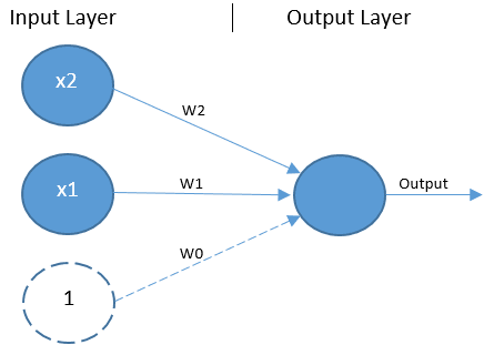
The perceptron is a type of feed-forward network, which means the process of generating an output — known as forward propagation — flows in one direction from the input layer to the output layer. There are no connections between units in the input layer. Instead, all units in the input layer are connected directly to the output unit.

A simplified explanation of the forward propagation process is that the input values X1 and X2, along with the bias value of 1, are multiplied by their respective weights W0..W2, and parsed to the output unit. The output unit takes the sum of those values and employs an activation function — typically the Heavside step function — to convert the resulting value to a 0 or 1, thus classifying the input values as 0 or 1.

It is the setting of the weight variables that gives the network’s author control over the process of converting input values to an output value. It is the weights that determine where the classification line, the line that separates data points into classification groups, is drawn. If all data points on one side of a classification line are assigned the class of 0, all others are classified as 1.

A limitation of this architecture is that it is only capable of separating data points with a single line. This is unfortunate because the XOR inputs are not linearly separable . This is particularly visible if you plot the XOR input values to a graph. As shown in figure 3, there is no way to separate the 1 and 0 predictions with a single classification line.

Multilayer Perceptrons

The solution to this problem is to expand beyond the single-layer architecture by adding an additional layer of units without any direct access to the outside world, known as a hidden layer. This kind of architecture — shown in Figure 4 — is another feed-forward network known as a multilayer perceptron (MLP).

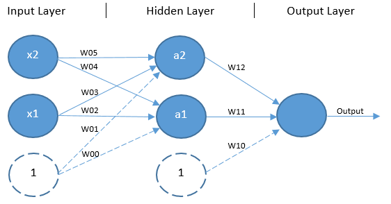
It is worth noting that an MLP can have any number of units in its input, hidden and output layers. There can also be any number of hidden layers. The architecture used here is designed specifically for the XOR problem.

Similar to the classic perceptron, forward propagation begins with the input values and bias unit from the input layer being multiplied by their respective weights, however, in this case there is a weight for each combination of input (including the input layer’s bias unit) and hidden unit (excluding the hidden layer’s bias unit). The products of the input layer values and their respective weights are parsed as input to the non-bias units in the hidden layer. Each non-bias hidden unit invokes an activation function — usually the classic sigmoid function in the case of the XOR problem — to squash the sum of their input values down to a value that falls between 0 and 1 (usually a value very close to either 0 or 1). The outputs of each hidden layer unit, including the bias unit, are then multiplied by another set of respective weights and parsed to an output unit. The output unit also parses the sum of its input values through an activation function — again, the sigmoid function is appropriate here — to return an output value falling between 0 and 1. This is the predicted output.

This architecture, while more complex than that of the classic perceptron network, is capable of achieving non-linear separation. Thus, with the right set of weight values, it can provide the necessary separation to accurately classify the XOR inputs.

Backpropagation

The elephant in the room, of course, is how one might come up with a set of weight values that ensure the network produces the expected output. In practice, trying to find an acceptable set of weights for an MLP network manually would be an incredibly laborious task. In fact, it is NP-complete (Blum and Rivest, 1992). However, it is fortunately possible to learn a good set of weight values automatically through a process known as backpropagation. This was first demonstrated to work well for the XOR problem by Rumelhart et al. (1985).

The backpropagation algorithm begins by comparing the actual value output by the forward propagation process to the expected value and then moves backward through the network, slightly adjusting each of the weights in a direction that reduces the size of the error by a small degree. Both forward and back propagation are re-run thousands of times on each input combination until the network can accurately predict the expected output of the possible inputs using forward propagation.

For the XOR problem, 100% of possible data examples are available to use in the training process. We can therefore expect the trained network to be 100% accurate in its predictions and there is no need to be concerned with issues such as bias and variance in the resulting model.

In this post, we explored the classic ANN XOR problem. The problem itself was described in detail, along with the fact that the inputs for XOR are not linearly separable into their correct classification categories. A non-linear solution — involving an MLP architecture — was explored at a high level, along with the forward propagation algorithm used to generate an output value from the network and the backpropagation algorithm, which is used to train the network.

The next post in this series will feature a implementation of the MLP architecture described here, including all of the components necessary to train the network to act as an XOR logic gate.

Blum, A. Rivest, R. L. (1992). Training a 3-node neural network is NP-complete. Neural Networks, 5(1), 117–127.

Minsky, M. Papert, S. (1969). Perceptron: an introduction to computational geometry. The MIT Press, Cambridge, expanded edition, 19(88), 2.

Rumelhart, D. Hinton, G. Williams, R. (1985). Learning internal representations by error propagation (No. ICS-8506). California University San Diego LA Jolla Inst. for Cognitive Science.

Top comments (3)

Templates let you quickly answer FAQs or store snippets for re-use.

• Joined Jun 17, 2021

Hey Jayesh. Nice post thank you! I would love to read the follow up with the implementation because I have problems of teaching MLP's simple relationships. I could not find that one here yet, so if you could provide me a link I would be more than happy.

• Joined Apr 13, 2024

• Joined Jun 11, 2022

Are you sure you want to hide this comment? It will become hidden in your post, but will still be visible via the comment's permalink .

Hide child comments as well

For further actions, you may consider blocking this person and/or reporting abuse

The Future of Information Retrieval: RAG Models vs. Generalized AI

Asad - May 31

How to Use ChatGPT to Kickstart Your Project and Begin Your Journey as a Programmer

Homayoun - Jun 1

CodeBehind Framework - Add Model in View

elanatframework - May 31

Instagram AI policy

Luke Cartwright - May 31

We're a place where coders share, stay up-to-date and grow their careers.

• Your cart is currently empty.
• Unlocking the Power of Neural Networks: Solving the XOR Problem with Ease

Neural networks have been proven to solve complex problems, and one of the most challenging ones is the XOR problem. In this article, we will explore how neural networks can solve this problem and provide a better understanding of their capabilities.

Understanding the XOR Problem in Neural Networks

As an AI expert, I have come across various problems that neural networks struggle to solve. One such problem is the XOR problem. The XOR (Exclusive OR) problem involves classifying input data into two classes based on their features. This may sound simple, but it’s not for traditional neural networks.

The XOR problem is a binary classification problem where the output is 1 if the inputs are different and 0 if they are the same. For example, if we have two inputs A and B, we want to classify them as follows:

Revolutionize Your Blogging Strategy with Content Automation Tools

Revolutionizing Content Creation: How AI Writers are Transforming the Blogging Industry

– If A = 0 and B = 0, then output = 0 – If A = 0 and B = 1, then output = 1 – If A = 1 and B = 0, then output = 1 – If A = 1 and B = 1, then output = 0

This problem may seem easy to solve manually, but it poses a challenge for traditional neural networks because they lack the ability to capture non-linear relationships between input variables.

Why Traditional Neural Networks Struggle to Solve the XOR Problem

Traditional neural networks use linear activation functions that can only model linear relationships between input variables. In other words, they can only learn patterns that are directly proportional or inversely proportional to each other.

For example, if we have two inputs X and Y that are directly proportional (i.e., as X increases, Y also increases), a traditional neural network can learn this relationship easily. However, when there is a non-linear relationship between input variables like in the case of the XOR problem, traditional neural networks fail to capture this relationship.

Traditional neural networks also use a single layer of neurons which makes it difficult for them to learn complex patterns in data. To solve complex problems like the XOR problem with traditional neural networks, we would need to add more layers and neurons which can lead to overfitting and slow learning.

Approaching the XOR Problem with Feedforward Neural Networks

One way to solve the XOR problem is by using feedforward neural networks. Feedforward neural networks are a type of artificial neural network where the information flows in one direction, from input to output.

Revolutionize Your Content with Our AI-Powered Blog Writing Service

Revolutionizing Content Creation: Multilingual AI Blog Service Launches

To solve the XOR problem with feedforward neural networks, we need to use non-linear activation functions such as sigmoid or ReLU (Rectified Linear Unit) that can capture non-linear relationships between input variables. We also need to use multiple layers of neurons to learn complex patterns in data.

Steps for Solving the XOR Problem with Feedforward Neural Networks

Step 1: define the network architecture.

The first step is to define the network architecture. For the XOR problem, we can use a network with two input neurons, two hidden neurons, and one output neuron.

Step 2: Initialize Weights and Biases

The next step is to initialize weights and biases randomly. This is important because it allows the network to start learning from scratch.

Revolutionizing Blogging: How Automated Content Creation is Changing the Game

Revolutionizing Blogging: How AI is Transforming Content Generation

Step 3: train the network.

The third step is to train the network using backpropagation algorithm. During training, we adjust weights and biases based on the error between predicted output and actual output until we achieve a satisfactory level of accuracy.

The Limitations of Single-Layer Feedforward Networks for Solving the XOR Problem

Although single-layer feedforward networks can solve some simple problems like linear regression, they are not suitable for solving complex problems like image recognition or natural language processing.

In fact, single-layer feedforward networks cannot solve problems that require non-linear decision boundaries like in the case of XOR problem. This is because they lack the ability to capture non-linear relationships between input variables.

Single-layer feedforward networks are also limited in their capacity to learn complex patterns in data. They have a fixed number of neurons which means they can only learn a limited number of features. To overcome this limitation, we need to use multi-layer feedforward networks.

Solving the XOR Problem with Multi-Layer Feedforward Neural Networks

Multi-layer feedforward neural networks, also known as deep neural networks, are artificial neural networks that have more than one hidden layer. These networks can learn complex patterns in data by using multiple layers of neurons.

To solve the XOR problem with multi-layer feedforward neural networks, we need to use multiple layers of non-linear activation functions such as sigmoid or ReLU. We also need to use backpropagation algorithm for training.

Steps for Solving the XOR Problem with Multi-Layer Feedforward Neural Networks

The first step is to define the network architecture. For the XOR problem, we can use a network with two input neurons, two hidden layers each with two neurons and one output neuron.

By using multi-layer feedforward neural networks, we can solve complex problems like image recognition or natural language processing that require non-linear decision boundaries.

How Backpropagation Helps in Solving the XOR Problem with Multi-Layer Feedforward Networks

Backpropagation is a supervised learning algorithm used to train neural networks. It is based on the chain rule of calculus and allows us to calculate the error at each layer of the network and adjust weights and biases accordingly.

In the case of multi-layer feedforward networks, backpropagation helps in solving the XOR problem by adjusting weights and biases at each layer based on the error between predicted output and actual output. This allows the network to learn complex patterns in data by using multiple layers of neurons.

Can Convolutional Neural Networks Solve the XOR Problem?

Convolutional neural networks (CNNs) are a type of artificial neural network that is commonly used for image recognition tasks. They use convolutional layers to extract features from images and pooling layers to reduce their size.

Although CNNs are not commonly used for solving simple problems like XOR problem, they can be adapted for this task by using one-dimensional convolutional layers instead of two-dimensional convolutional layers.

However, it’s important to note that CNNs are designed for tasks like image recognition where there is spatial correlation between pixels. For simple problems like XOR problem, traditional feedforward neural networks are more suitable.

Revolutionize Your Blogging with the Latest AI Writing Tool!

Revolutionizing Content Creation: AI-Powered Blogging Platform Takes the Internet by Storm

Differences between recurrent and feedforward neural network approaches to solving the xor problem.

Recurrent neural networks (RNNs) are a type of artificial neural network that can process sequential data such as time-series or natural language data. Unlike feedforward neural networks, RNNs have feedback connections that allow them to store information from previous time steps.

To solve the XOR problem with RNNs, we need to use a special type of RNN called Long Short-Term Memory (LSTM). LSTMs have memory cells that can store information over long periods of time which makes them suitable for processing sequential data.

The main difference between feedforward and recurrent approaches to solving XOR problem is that feedforward networks use fixed-size input and output vectors while RNNs can process sequences of varying length.

Challenges Associated with Using Recurrent Neural Networks for Solving the XOR Problem

Although RNNs are suitable for processing sequential data, they pose a challenge when it comes to solving the XOR problem. This is because XOR problem requires memorizing information over long periods of time which is difficult for RNNs.

RNNs suffer from the vanishing gradient problem which occurs when the gradient becomes too small to update weights and biases during backpropagation. This makes it difficult for them to learn long-term dependencies in data.

To overcome this challenge, we need to use LSTM architecture which has memory cells that can store information over long periods of time.

The Role of Long Short-Term Memory (LSTM) Architecture in Solving the XOR Problem with Recurrent Neural Networks

Long Short-Term Memory (LSTM) is a special type of recurrent neural network that has memory cells that can store information over long periods of time. LSTMs are designed to solve problems where there are long-term dependencies in data.

To solve the XOR problem with LSTMs, we need to use a network with one input neuron, two hidden layers each with four LSTM neurons, and one output neuron. During training, we adjust weights and biases based on the error between predicted output and actual output until we achieve a satisfactory level of accuracy.

By using LSTMs, we can solve complex problems like natural language processing or speech recognition that require memorizing information over long periods of time.

Other Types of Neural Network Architectures for Solving the XOR Problem

Apart from feedforward, convolutional, and recurrent neural networks, there are other types of neural network architectures that can be used for solving the XOR problem. These include:

– Autoencoder neural networks: These are neural networks that are trained to reconstruct their input data. They can be used for feature extraction and anomaly detection.

– Radial basis function (RBF) neural networks: These are neural networks that use radial basis functions as activation functions. They can be used for clustering and classification tasks.

– Self-organizing maps (SOMs): These are unsupervised learning algorithms that can be used for clustering and visualization of high-dimensional data.

The Role of Transfer Learning in Solving Complex Problems Like the XOR Problem

Transfer learning is a technique where we use pre-trained models to solve new problems. It involves using the knowledge learned from one task to improve the performance of another related task.

In the case of XOR problem, transfer learning can be applied by using pre-trained models on similar binary classification tasks. For example, if we have a pre-trained model on classifying images as cats or dogs, we can use this model as a starting point for solving the XOR problem.

Revolutionizing Content Creation: The Rise of Automated Blog Writing Software

Revolutionizing Content Creation: How AI is Streamlining Blog Post Automation

Transfer learning reduces the amount of training data required and speeds up the training process. It also improves the accuracy of models by leveraging knowledge learned from related tasks.

Using Unsupervised Learning Techniques to Solve the XOR Problem Without Labeled Data

Unsupervised learning is a type of machine learning where we train models on unlabeled data. It involves finding patterns in data without any prior knowledge about their labels or categories.

In the case of XOR problem, unsupervised learning techniques like clustering or dimensionality reduction can be used to find patterns in data without any labeled examples. For example, we can use k-means clustering algorithm to group input data into two clusters based on their features.

However, unsupervised learning techniques may not always provide accurate results compared to supervised learning techniques that rely on labeled examples.

Practical Applications of Solving the XOR Problem Using Neural Networks

Although XOR problem may seem like a simple problem, it has practical applications in various fields such as:

– Cryptography: XOR is commonly used in encryption algorithms to scramble data.

– Robotics: XOR can be used to control robotic arms and legs based on sensory input.

– Finance: XOR can be used for fraud detection by classifying transactions as fraudulent or non-fraudulent based on their features.

The Limitations and Drawbacks of Using Neural Networks for Solving Problems Like the XOR Problem

Although neural networks have shown great promise in solving complex problems, they have limitations and drawbacks that need to be considered. Some of these include:

– Overfitting: Neural networks can overfit training data which leads to poor generalization on new data.

– Slow learning: Training large neural networks can take a long time due to the large number of parameters involved.

– Black box models: Neural networks are often considered black box models because it’s difficult to interpret how they arrive at their predictions.

– Lack of transparency: Due to their complexity, neural networks lack transparency which makes it difficult for humans to understand how they work.

Despite these limitations, neural networks remain an important tool for solving complex problems in various fields.

In conclusion, neural networks have proven to be a powerful tool in solving the XOR problem. With their ability to learn and adapt, they can tackle complex tasks that traditional programming methods struggle with. If you’re interested in exploring the possibilities of AI for your business or project, don’t hesitate to get in touch with us and check out our AI services. We’re always happy to help!

https://www.researchgate.net/publication/346707273/figure/fig2/AS:11431281104506106@1670094751465/The-Running-Time-on-Random-S-boxes_Q320.jpg

How neural network solves the XOR problem?

To solve the XOR problem using neural networks, one can use either Multi-Layer Perceptrons or a neural network that consists of an input layer, a hidden layer, and an output layer. As the neural network processes data through forward propagation, the weights of each layer are adjusted accordingly and the XOR logic is executed.

Why is the XOR problem interesting to neural network researchers?

Neural network researchers find the XOR problem particularly intriguing because it is a complicated binary function that cannot be resolved by a neural network.

https://www.researchgate.net/publication/346705804/figure/fig1/AS:11431281104839310@1670267196273/Schematics-of-Arbiter-PUF-XOR-Arbiter-PUF-and-Interpose-PUF_Q320.jpg

How many neurons does it take to solve XOR?

The XOR problem can be solved using just two neurons, according to a statement made on January 18th, 2017.

How do neural networks solve problems?

Artificial neural networks are a type of machine learning algorithm inspired by the structure of the human brain. They can solve problems using trial and error, without being explicitly programmed with rules to follow. These algorithms are part of a larger category of machine learning techniques.

Can decision trees solve the XOR problem?

It is feasible to utilize decision trees to execute the XOR operation, as of October 4th, 2019.

Why can t the XOR problem be solved by a one layer perceptron?

The perceptron is limited to being able to handle only linearly separable data and cannot replicate the XOR function.

• Martin Thoma

XOR tutorial with TensorFlow

The XOR-Problem is a classification problem, where you only have four data points with two features. The training set and the test set are exactly the same in this problem. So the interesting question is only if the model is able to find a decision boundary which classifies all four points correctly.

Neural Network basics

I think of neural networks as a construction kit for functions. The basic building block - called a "neuron" - is usually visualized like this:

It gets a variable number of inputx \(x_0, x_1, \dots, x_n\) , they get multiplied with weights \(w_0, w_1, \dots, w_n\) , summed and a function \(\varphi\) is applied to it. The weights is what you want to "fine tune" to make it actually work. When you have more of those neurons, you visualize it like this:

In this example, it is only one output and 5 inputs, but it could be any number. The number of inputs and outputs is usually defined by your problem, the intermediate is to allow it to fit more exact to what you need (which comes with some other implications).

Now you have some structure of the function set, you need to find weights which work. This is where backpropagation 3 comes into play. The idea is the following: You took functions ( \(\varphi\) ) which were differentiable and combined them in a way which makes sure the complete function is differentiable. Then you apply an error function (e.g. the euclidean distance of the output to the desired output, Cross-Entropy) which is also differentiable. Meaning you have a completely differentiable function. Now you see the weights as variables and the data as given parameters of a HUGE function. You can differentiate (calculate the gradient) and go from your random weights "a step" in the direction where the error gets lower. This adjusts your weights. Then you repeat this steepest descent step and hopefully end up some time with a good function.

For two weights, this awesome image by Alec Radford visualizes how different algorithms based on gradient descent find a minimum ( Source with even more of those):

So think of back propagation as a shortsighted hiker trying to find the lowest point on the error surface: He only sees what is directly in front of him. As he makes progress, he adjusts the direction in which he goes.

Targets and Error function

First of all, you should think about how your targets look like. For classification problems, one usually takes as many output neurons as one has classes. Then the softmax function is applied. 1 The softmax function makes sure that the output of every single neuron is in \([0, 1]\) and the sum of all outputs is exactly \(1\) . This means the output can be interpreted as a probability distribution over all classes.

Now you have to adjust your targets. It is likely that you only have a list of labels, where the \(i\) -th element in the list is the label for the \(i\) -th element in your feature list \(X\) (or the \(i\) -th row in your feature matrix \(X\) ). But the tools need a target value which fits to the error function. The usual error function for classification problems is cross entropy (CE). When you have a list of \(n\) features \(x\) , the target \(t\) and a classifier \(clf\) , then you calculate the cross entropy loss for this single sample by:

Now we need a target value for each single neuron for every sample \(x\) . We get those by so called one hot encoding : The \(k\) classes all have their own neuron. If a sample \(x\) is of class \(i\) , then the \(i\) -th neuron should give \(1\) and all others should give \(0\) . 2

sklearn provides a very useful OneHotEncoder class. You first have to fit it on your labels (e.g. just give it all of them). In the next step you can transform a list of labels to an array of one-hot encoded targets:

Install Tensorflow

The documentation about the installation makes a VERY good impression. Better than anything I can write in a few minutes, so ... RTFM 😜

For Linux systems with CUDA and without root privileges, you can install it with:

But remember you have to set the environment variable LD_LIBRARY_PATH and CUDA_HOME . For many configurations, adding the following lines to your .bashrc will work:

I currently (19.07.2016) to use Tensorflow rc0.7 ( installation instructions ) with CUDA 7.5 ( installation instructions ). I had a couple of problems with other versions (e.g. #3342 , #2810 , #2034 , but that might only have been bad luck. Who knows.).

Tensorflow basics

Tensorflow helps you to define the neural network in a symbolic way. This means you do not explicitly tell the computer what to compute to inference with the neural network, but you tell it how the data flow works. This symbolic representation of the computation can then be used to automatically caluclate the derivates. This is awesome! So you don't have to make this your own. But keep it in mind that it is only symbolic as this makes a few things more complicated and different from what you might be used to.

Tensorflow has placeholders and variables . Placeholders are the things in which you later put your input. This is your features and your targets, but might be also include more. Variables are the things the optimizer calculates.

Now you should be able to understand the following code which solves the XOR problem. It defines a neural network with two input neurons, 2 neurons in a first hidden layer and 2 output neurons. All neurons have biases.

The output is:

The resulting decision boundary looks like this:

I recommend reading the Tensorflow Whitepaper if you want to understand Tensorflow better.

Softmax is similar to the sigmoid function, but with normalization.  ↩

Actually, we don't want this. The probability of any class should never be exactly zero as this might cause problems later. It might get very very small, but should never be 0.  ↩

Backpropagation is only a clever implementation of gradient descent. It belongs to the bigger class of iterative descent algorithms.  ↩

• Machine Learning 81
• Tensorflow 3

How to build a neural network on Tensorflow for XOR

We bring to your attention another article on neural networks and their practical application. This article will look at a classic example for learning the neural network of the XOR function. There are already quite a large number of such manuals on the Internet, so the purpose of this text will be as follows:

• use the XOR function with two inputs and one output for a demo
• use tensors to build a mathematical model of a neural network
• use Python for programming as a simple and common language
• make the code as simple and straightforward as possible
• train the neural network in several ways.

Table of contents:

What is a neural network, what is xor, why use tensorflow.

• Basic of matrix operation.
• Gradient descent.
• Building and training XOR neural network.
• Test the solution.
• Using different optimizer.
• Conclusion.

Artificial neural networks (ANNs), or connectivist systems are computing systems inspired by biological neural networks that make up the brains of animals. Such systems learn tasks (progressively improving their performance on them) by examining examples, generally without special task programming.

ANN is based on a set of connected nodes called artificial neurons (similar to biological neurons in the brain of animals). Each connection (similar to a synapse) between artificial neurons can transmit a signal from one to the other. The artificial neuron receiving the signal can process it and then signal to the artificial neurons attached to it.

In common implementations of ANNs, the signal for coupling between artificial neurons is a real number, and the output of each artificial neuron is calculated by a nonlinear function of the sum of its inputs.

Neural networks are now widespread and are used in practical tasks such as speech recognition, automatic text translation, image processing, analysis of complex processes and so on. 

Fig. 1. Biological and neural networks.

Image source

XOR is an exclusive or (exclusive disjunction) logical operation that outputs true only when inputs differ.

This operation can be represented as

Or by input values, XOR gives the following truth table.

In the book “Perceptrons: an Introduction to Computational Geometry” (published in 1969), Marvin Minsky and Seymour Papert, show that neural network with one neuron cannot solve the XOR problem.

Fig. 2. How to draw one line to divide green points from red points? None.

One neuron with two inputs can form a decisive surface in the form of an arbitrary line. In order for the network to implement the XOR function specified in the table above, you need to position the line so that the four points are divided into two sets. Trying to draw such a straight line, we are convinced that this is impossible. This means that no matter what values are assigned to weights and thresholds, a single-layer neural network is unable to reproduce the relationship between input and output required to represent the XOR function.

TensorFlow is an open-source machine learning library designed by Google to meet its need for systems capable of building and training neural networks and has an Apache 2.0 license.

Created by the Google Brain team, TensorFlow presents calculations in the form of stateful dataflow graphs. The library allows you to implement calculations on a wide range of hardware, from consumer devices running Android to large heterogeneous systems with multiple GPUs. TensorFlow allows you to transfer the performance of computationally intensive tasks from a single CPU environment to a heterogeneous fast environment with multiple GPUs without significant code changes TensorFlow is designed to provide massive concurrency and highly scalable machine learning for a wide range of users.

The central object of TensorFlow is a dataflow graph representing calculations. The vertices of the graph represent operations, and the edges represent tensors (multidimensional arrays that are the basis of TensorFlow). The data flow graph as a whole is a complete description of the calculations that are implemented within the session and performed on CPU or GPU devices.

Assuming you have python3 and pip3 on your computer, to install Tensorflow you need to type in the command line:

And to verify installation type:

Yes, it works. Now let’s install Jupyter notebook. Jupyer notebook will help to enter code and run it in a comfortable environment.

And run Jupyter:

You will have a new window in your browser and will be ready to write code in Python with TensorFlow.

Additional information for installing Tensorflow on your operating system can be found here .

Basic of matrix operation

Let’s review the basic matrix operation that is required to build a neural network in TensorFlow.

C = A*B , where A and B are matrixes. The matrix A with a size of l x m and matrix B with a size m x n and result matrix C with size l x m .

Ax = b , where A is a matrix, x and b are vectors. The number of columns in A should be the same as the number of elements in vectors x and b .

The classic multiplication algorithm will have complexity as O(n3).

Gradient descent

A large number of methods are used to train neural networks, and gradient descent is one of the main and important training methods. It consists of finding the gradient, or the fastest descent along the surface of the function and choosing the next solution point. An iterative gradient descent finds the value of the coefficients for the parameters of the neural network to solve a specific problem.

Gradient descent is an iterative optimization algorithm for finding the minimum of a function. To find the minimum of a function using gradient descent, we can take steps proportional to the negative of the gradient of the function from the current point.

To train the neural network, we build the error function. The error function is calculated as the difference between the output vector from the neural network with certain weights and the training output vector for the given training inputs.

If we change weights on the next step of gradient descent methods, we will minimize the difference between output on the neurons and training set of the vector. As a result, we will have the necessary values of weights and biases in the neural network and output values on the neurons will be the same as the training vector.

Of course, there are some other methods of finding the minimum of functions with the input vector of variables, but for the training of neural networks gradient methods work very well. They allow finding the minimum of error (or cost) function with a large number of weights and biases in a reasonable number of iterations. A drawback of the gradient descent method is the need to calculate partial derivatives for each of the input values. Very often when training neural networks, we can get to the local minimum of the function without finding an adjacent minimum with the best values. Also, gradient descent can be very slow and makes too many iterations if we are close to the local minimum.

Fig. 3. Gradient descent method. Image source

Let's look at a simple example of using gradient descent to solve an equation with a quadratic function.

We need to find a value of a = 4 (approximately) by gradient descent. We have one variable x in this function and gradient will look like y’= 8 x and TensorFlow can calculate it automatically under the hood.

So, the answer is equal to  3.9999995 with 100 iterations on TensorFlow gradient descent. If we will make more than 50 iterations, the result will be more accurate.

Building and training XOR neural network

Now let's build the simplest neural network with three neurons to solve the XOR problem and train it using gradient descent.

If we imagine such a neural network in the form of matrix-vector operations, then we get this formula.

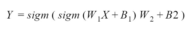
Where: 

• X is an input value vector, size 2x1 elements
• W1 is a matrix of the coefficient for the first layer, size 2x2 elements
• B1 is a bias for the first layer, a vector with 2x1 elements
• W2  is a vector of the coefficient for the first layer, size 2x1 elements
• B2 is a value of bias for the second layer, size 1x1 element
• Y is an output value, size 1x1 element
• sigm(x) is a sigmoid activation function for neural network

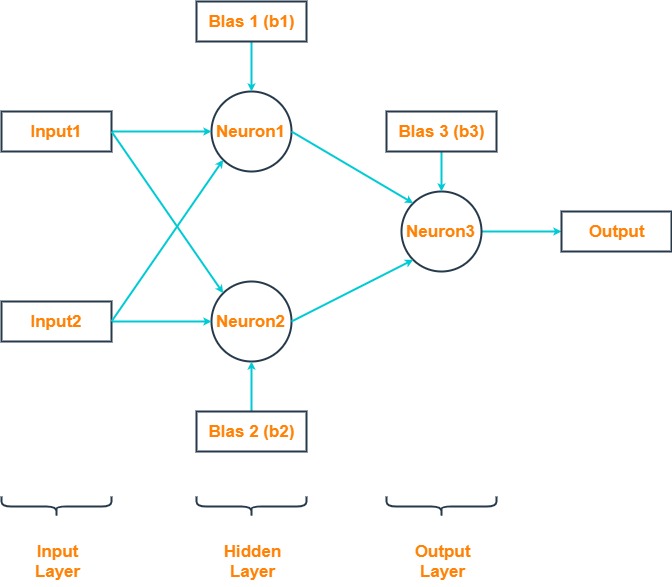
Test the solution

And now let's run all this code, which will train the neural network and calculate the error between the actual values of the XOR function and the received data after the neural network is running. The closer the resulting value is to 0 and 1, the more accurately the neural network solves the problem.

And so we see that for 100,000 iterations we got an error of 0.0005582984 and the output values are close to 0 and 1 . That is, the neural network coped with its task.

Using different optimizer

Now let's change one line in the code. Replace the gradient descent with the Adam optimizer.

And we will have a significantly better result. When using Adam's optimizer, we get the result of a neural network in just 1000 iterations and with error 8.665349e-05 . 

Adam’s optimizer was presented by Diederik Kingma from OpenAI and Jimmy Ba from the University of Toronto in their 2015 ICLR paper ” Adam: A Method for Stochastic Optimization ”. Adam is an algorithm that is a first-order method based on adaptive estimates of lower-order moments. This method implements the benefits of two other methods AdaGrad and RMSProp. The algorithm calculates an exponential moving average of the gradient and the squared gradient. It is highly recommended for training deep learning networks.

And so, what we did get as a result? It turns out that TensorFlow is quite simple to install and matrix calculations can be easily described on it. The beauty of this approach is the use of a ready-made method for training a neural network. The article provides a separate piece of TensorFlow code that shows the operation of the gradient descent. This facilitates the task of understanding neural network training . A slightly unexpected result is obtained using gradient descent since it took 100,000 iterations, but Adam's optimizer copes with this task with 1000 iterations and gets a more accurate result.

We wish you successful projects with TensorFlow.

Related articles

Let's discuss your project

We look forward to learning more and consulting you about your product idea or helping you find the right solution for an existing project.

Your message is received. Svitla's sales manager of your region will contact you to discuss how we could be helpful.

Navigation Menu

Search code, repositories, users, issues, pull requests..., provide feedback.

We read every piece of feedback, and take your input very seriously.

Saved searches

Use saved searches to filter your results more quickly.

To see all available qualifiers, see our documentation .

xor-neural-network

Here are 37 public repositories matching this topic..., dlidstrom / neuralnetworkinalllangs.

Vanilla neural network implemented in all major languages

• Updated Jan 31, 2024

Frixoe / xor-neural-network

A simple Neural Network that learns to predict the XOR logic gates.

• Updated Mar 6, 2018
• Jupyter Notebook

shayanalibhatti / Coding-neural_network-for-XOR-logic-from-scratch

In this repository, I implemented a proof of concept of all my theoretical knowledge of neural network to code a simple neural network for XOR logic function from scratch without using any machine learning library

• Updated Jul 26, 2020

reddragonnm / neatpy

A NEAT library in Python

• Updated Jun 4, 2022

neemiasbsilva / machine-learning-algorithm

Some algorithms of machine learning like Regression, Cluster, Deep Learning, and much more.

• Updated Nov 20, 2022

sushantPatrikar / XOR-Gate-With-Neural-Network-Using-Numpy

XOR gate which predicts the output using Neural Network 🔥

• Updated Aug 4, 2019

prakHr / NeuralNetworksAndFuzzyLogic

[College Course] - Course: BITS F312 Neural Network and Fuzzy Logic

Nikronic / Artificial-Neural-Networks

Projects of the course Artificial Neural Networks by Dr. Mozayani - Fall 2019

• Updated Mar 16, 2020

Vinetos / neural-network-xor

Implements a neural network learning XOR gate in your favourite languages !

• Updated Oct 10, 2020

IvanovskyOrtega / Neural-Networks

Many different Neural Networks in Python Language. This repository is an independent work, it is related to my 'Redes Neuronales' repo, but here I'll use only Python.

• Updated Mar 10, 2019

9rince / neural_nets

exercises with neural nets

• Updated Aug 23, 2018

kinoute / l-layers-xor-neural-network

A L-Layers XOR Neural Network using only Python and Numpy that learns to predict the XOR logic gates.

• Updated Jun 24, 2019

vernikagupta / Deep_Learning_with_Maths

Complete introduction to deep learning with various architechtures. Maths involved is also included. Code samples for building architechtures is included using keras. This repo also includes implementation of Logical functions AND, OR, XOR.

• Updated Dec 8, 2022

melchisedech333 / xor-neural-network

🤖 Artificial intelligence (neural network) proof of concept to solve the classic XOR problem. It uses known concepts to solve problems in neural networks, such as Gradient Descent, Feed Forward and Back Propagation.

• Updated Oct 17, 2022

cgera13 / XOR-Neural-Network

Simulation of an XOR neural network that provides 100% classification using the Backpropagation learning algorithm

• Updated Feb 6, 2018

UtkarshAgrawalDTU / XOR-NeuralNetwork

Implementation of XOR Logic Gate using Simple Neural Network (Algorithm : Gradient Descent)

• Updated Aug 16, 2019

viktorlott / NeuralNetwork

My First homemade neural network

• Updated Oct 31, 2023

gentaiscool / multi-layer-perceptron

Implementation of multi-layer perceptron neural network

• Updated May 29, 2018

yashsmehta / XOR-jax

Simple toy neural networks in JAX solving XOR

• Updated Aug 21, 2022

DavidCoroama / xorai

A basic neural network written in C++ that can calculate the expected output of an xor between two numbers.

• Updated Nov 9, 2023

Improve this page

Add a description, image, and links to the xor-neural-network topic page so that developers can more easily learn about it.

Curate this topic

Add this topic to your repo

To associate your repository with the xor-neural-network topic, visit your repo's landing page and select "manage topics."

An official website of the United States government

The .gov means it’s official. Federal government websites often end in .gov or .mil. Before sharing sensitive information, make sure you’re on a federal government site.

The site is secure. The https:// ensures that you are connecting to the official website and that any information you provide is encrypted and transmitted securely.

• Publications
• Account settings

Preview improvements coming to the PMC website in October 2024. Learn More or Try it out now .

• Advanced Search
• Journal List
• Comput Intell Neurosci
• v.2022; 2022

Single Neuron for Solving XOR like Nonlinear Problems

Ashutosh mishra.

School of Integrated Technology, YICT, Yonsei University, Seoul, Republic of Korea

Jaekwang Cha

Associated data.

The data used to support the findings of this study are included in the article.

XOR is a special nonlinear problem in artificial intelligence (AI) that resembles multiple real-world nonlinear data distributions. A multiplicative neuron model can solve these problems. However, the multiplicative model has the indigenous problem of backpropagation for densely distributed XOR problems and higher dimensional parity problems. To overcome this issue, we have proposed an enhanced translated multiplicative single neuron model. It can provide desired tessellation surface. We have considered an adaptable scaling factor associated with each input in our proposed model. It helps in achieving optimal scaling factor value for higher dimensional input. The efficacy of the proposed model has been tested by randomly increasing input dimensions for XOR-type data distribution. The proposed model has crisply classified even higher dimensional input in their respective class. Also, the computational complexity is the same as that of the previous multiplicative neuron model. It has shown more than an 80% reduction in absolute loss as compared to the previous neuron model in similar experimental conditions. Therefore, it can be considered as a generalized artificial model (single neuron) with the capability of solving XOR-like real problems.

1. Introduction

Minski and Perpert deduced that the XOR problem requires more than one hyperplane [ 1 ]. They provide a more generalized artificial neuron model by introducing the concept of weights and proved the inability of a single perceptron for solving ‘Exclusive-OR (XOR)' [ 2 ]. The XOR problem is symmetrical to other popular and real-world problems such as XOR type nonlinear data distribution in two classes, N -bit parity problems. [ 3 ]. Therefore, many researchers tried to find a suitable way out to solve the XOR problem [ 4 – 15 ]. Although, most of the solutions are for the classical XOR problem. They either use more than one layer or provide a complex solution for two-bit logical XOR only. Few of these used the complex value neuron model, eventually creating one more layer (i.e., hidden layer). Because the complex value neuron model requires representing the real input in a complex domain, one approach is based on the multiplicative neuron model. This is translated multiplicative neuron ( π t -neuron) approach [ 16 , 17 ]. They have modified the π -neuron model (which generates the decision surfaces centered at the origin of input) to an extended multiplicative neuron, i.e., a π t -neuron model for solving the N -bit parity problems by creating tessellation surfaces. However, it has limitations for higher dimensional N -bit parity problems. It is suitable for up to six dimensions. For seven and higher dimensional inputs, it has reported poor accuracy [ 17 ]. In other words, it has a convergence problem for higher dimensional inputs. It is merely because of the multiplicative nature of the model. More clearly, the infinitesimal errors in the model obtain a much smaller value after getting multiplied in case of higher dimensional inputs, consequently vanishing the gradient. Therefore, a convergence problem occurs in this model for higher-dimensional inputs.

To overcome the issue of the π t -neuron model, we have proposed an enhanced translated multiplicative model neuron ( π t -neuron) model in this paper. It helps in achieving mutually orthogonal separation in the case of two-bit classical XOR data distribution. Also, the proposed model has shown the capability for solving the higher-order N -bit parity problems. Therefore, it is a generalized artificial model for solving real XOR problems. To examine this claim, we have tested our model on different XOR data distributions and N -bit parity problems. For parity problems, we have varied the input dimension for a higher dimensional dataset. Our proposed model has no vanishing gradient issues and convergence issues for higher dimensional inputs. The proposed model has accurately classified the considered dataset. Table 1 presents the list of variables used in this article with their meaning.

List of variables used in this article with their meaning.

2. Understanding the XOR Problem

XOR is a classical problem in the artificial neural network (ANN) [ 18 ]. The digital two-input XOR problem is represented in Figure 1 . By considering each input as one dimension and mapping the digital digit ‘ 0 ' as the negative axis and ‘ 1 ' as the positive axis, the same two-digit XOR problem becomes XOR type nonlinear data distribution in two-dimensional space. It is obvious here that the classes in two-dimensional XOR data distribution are the areas formed by two of the axes ‘ X 1 ' and ‘ X 2 ' (Here, X 1 is input 1 , and X 2 is input 2 ). Furthermore, these areas represent respective classes simply by their sign (i.e., negative area corresponds to class 1 , positive area corresponds to class 2 ).

XOR problem is illustrated by considering each input as one dimension and mapping the digital digit ‘ 0 ' as negative axis and ‘ 1 ' as the positive axis. Therefore, XOR data distribution is the areas formed by two of the axes ‘ X 1 ' and ‘ X 2 ', such that the negative area corresponds to class 1 , and the positive area corresponds to class 2 .

There are many other nonlinear data distributions resembling XOR. N -bit parity problem is one such typical example. Both these problems are popular in the AI research domain and require a generalized single neuron model to solve them. We have seen that these problems require a model which can distinguish between positive and negative quantities. Interestingly, addition cannot easily separate positive and negative quantities, whereas multiplication has the basic property to distinguish between positive and negative quantities. Therefore, previous researchers suggested using a multiplicative neuron model for solving XOR and similar problems.

3. Translated Multiplicative Neuron (Π T -NEURON) Model

The idea of the multiplicative neuron model was initiated by Durbin et al. in 1989 [ 19 ]. They named this model the ‘ Product Units (PUs) ' and used this model to deal with the generalized polynomial terms in the input. It can learn higher-order inputs easily as compared to the additive units. This is because of its increased information capacity as compared to the additive units [ 19 ]. Though, PU has shown the capability for N -bit parity problems. However, it has issues in training with the standard backpropagation (BP) algorithm especially for higher-order inputs (more than three-dimensional input) [ 20 ]. According to Leerink et al., it is because of nonglobal minima trapping in the case of higher dimensional inputs [ 20 ]. Later, in 2004, Iyoda et al. proposed a single neuron based on a multiplicative neuron model, aka π t -neuron model, to solve the XOR and parity bit problems [ 16 , 17 ]. They have modified the previous multiplicative π -neuron model to find a suitable tessellation decision surface. They incorporated a scaling factor, a threshold value, and used the sigmoid as an activation function to solve the N -bit parity problems using a single translated multiplicative neuron (the model is defined by equations ( 1 ) and ( 2 )) [ 16 ].

Here, ‘ v π ‒t ' represents the π t -neuron model mathematically, ‘ y ' is the final output through the activation function ‘ f ', ‘ b π‒t ' is scaling factor, and ‘ t i ' represent the coordinates of the center of the decision surfaces [ 16 ]. Mathematically, Iyoda et al. have shown the capability of the model for solving the logical XOR and N -bit parity problems for ∀ N  ≥ 1. However, this model also has a similar issue in training for higher-order inputs.

3.1. Limitations of Translated Multiplicative Neuron

The π t -neuron model has shown the appropriate research direction for solving the logical XOR and N -bit parity problems [ 16 ]. The reported success ratio is ‘1' for two-bit to six-bit inputs in [ 17 ]. However, in the case of seven-bit input, the reported success ratio is ‘0.6' only. Success ratio has been calculated by considering averaged values over ten simulations [ 17 ]. Also, for successful training in the case of seven-bit, it requires adjusting the trainable parameter (scaling factor b π‒t ) [ 17 ]. This is also indicating the training issue in the case of higher dimensional inputs. Moreover, Iyoda et al. have suggested increasing the range of initialization for scaling factors in case of a seven-bit parity problem [ 17 ]. Although, after the suggested increment as well, the reported success ratio is ‘0.6' only [ 17 ]. It indicates the problem of training in the π t -neuron model for higher dimensional input.

3.2. Causes of Failure in Π t -NEURON Model

In the backpropagation algorithm, the local gradient ‘ δ ( n )' accounts for the required changes in the trainable parameter at ‘ n th ' iteration to obtain desired output [ 21 ]. It is equal to the product of the corresponding error signal for that neuron and the derivative of the associated activation function [ 21 ]. Backpropagation requires that the activation function should be bounded, continuous, and monotonic. Also, it should be continuously differentiable for the entire domain of the input to get optimization [ 22 ]. Sigmoid activation function ‘ ϕ ( x )' is preferred in the classification problem because it has met all of the aforementioned requirements [ 23 ]. Also, it is an appropriate activation function for training multiplicative neuron models [ 23 ]. Iyoda et al. have demonstrated the error gradient (∇ Ɛ ) associated with the π t -neuron model [ 17 ]. Here, ‘ Ɛ ( n )' is the error energy, i.e., the instantaneous sum of the error squares at ‘ n th ' iteration. The error gradient has two components, one is due to the scaling factor ‘( b π‒t ),' given by equation ( 3 ), and the other is due to the thresholds ‘ t i ', given by equation ( 4 ) [ 17 ].

Here, ‘ n ' represents ‘ n th ' iteration, ∀ ( k  =  1 , 2 , 3 ,…, N ). ‘ x k ( n )' is the ‘ k th ' input for ‘ n th ' iteration, and ‘ v π ‒t ( n )' represents π t -neuron model. Therefore, the error's gradient obtains a much smaller value after getting multiplied for higher dimensional inputs and becomes an infinitesimally small value. Consequently, vanishing the gradient. Therefore, a convergence problem occurs in this model.

It is inferred from Figure 1 and equation ( 1 ) that the π t -neuron model has ranged between [‒1, 1] for XOR and N -bit parity problems. Here, ‘ ‒1 ' corresponds to digit ‘ 0 ', and ‘ +1 ' corresponds to digit ‘ 1 '. Sigmoid function has a basic issue of vanishing gradient near the extremes as shown in Figure 2(a) . However, about the XOR and N -bit parity problems, the input varies between [‒1, 1] only, as explained earlier. Therefore, the main region of interest is incorporated by a rectangular box of sigmoid activation function in Figure 2 . Here, it is important to notice that margin between two points has been reduced by the sigmoid activation function (as shown in Figure 2(a) , ϕ (‒1) = 0.2689, and ϕ (1) = 0.7311). Therefore, it leads to the smaller local gradient ‘ δ ( n )' value (given by Equation ( 5 )) which consequently results in smaller error gradients (given equations ( 3 )–( 5 )), eventually leading to the gradient vanishing problem.

(a) Sigmoid function ϕ(x) ; (b) effect of scaling on ϕ(x) .

For higher dimensional input, the error gradient (∇ Ɛ ) attains further smaller values because of the presence of the factor (∏ ( x k ( n ) +  t k ( n ))) in the expression of error gradients (as given by equations ( 3 )–( 5 )). Therefore, the possibilities of nonconvergence/nonglobal minima problems occur in the previous π t -neuron model. To overcome this issue, the model should have a larger margin for the extreme values. It is possible by introducing a compensatory scaling factor in the model. It eventually scales the sigmoid activation function, as depicted in Figure 2(b) . Therefore, in [ 17 ], the author suggested using a scaling factor ‘ b π‒t '. However, it requires an optimized value of the scaling factor to mitigate the effect of multiplication and sigmoid function in higher-dimensional problems. Because the effect of multiplication and sigmoid function is severe in higher-order input, Iyoda et al. recommended initializing the scaling factor only with higher values (not to the threshold factor) for the seven-bit parity problem [ 17 ]. Convergence is not possible with a smaller scaling factor for the higher dimensional problem (results given in ‘Table 2' of [ 17 ] follow this statement). Though, the idea of increasing the learning rate for the scaling factor is worth overcoming the vanishing gradient problem in higher dimensional input. However, an optimized value of the learning rate is not suggested in the previous π t -neuron model. Also, it is difficult to adjust the appropriate learning rate or range of initialization of scaling factors for variable input dimensions. Therefore, a generalized solution is still required to solve these issues of the previous model. In this paper, we have suggested a generalized model for solving the XOR and higher-order parity problems by enhancing the p t -neuron model.

4. Related Works

Robotics, parity problems, and nonlinear time-series prediction are some of the significant problems suggested by the previous researchers where multiplicative neurons are applied. Forecasting involving the time series has been performed using the multiplicative neuron models [ 24 – 26 ]. Yildirim et al. have proposed a threshold single multiplicative neuron model for time series prediction [ 24 ]. They utilized a threshold value and used the particle swarm optimization (PSO) and harmony search algorithm (HSA) to obtain the optimum weight, bias, and threshold values. In [ 25 ], Yolcu et al. have used autoregressive coefficients to predict the weights and biases for time series modeling. A recurrent multiplicative neuron model was presented in [ 26 ] for forecasting time series.

Yadav et al. have also used a single multiplicative neuron model for time series prediction problems [ 27 ]. In [ 28 ], authors have used the multiplicative neuron model for the prediction of terrain profiles for both air and ground vehicles. Egrioglu et al. have represented forecasting purposes like classical time series forecasting using a single multiplicative neuron model in [ 29 ]. In [ 30 ], Gao et al. proposed a dendritic neuron model to overcome the limitation of traditional ANNs. It has utilized the nonlinearity of synapses to improve the capability of artificial neurons. A few other recent works are suggested in [ 31 – 35 ].

5. Enhanced Translated Multiplicative Neuron

We have seen the problems associated with the π t -neuron model. It has an issue with BP training in case of highly dense XOR data distribution and higher dimensional parity problems. In this paper, we have proposed an enhanced translated multiplicative single neuron model which can easily learn the nonlinear problems such as XOR and N -bit parity without any training limitations. We have modified the existing π t -neuron to overcome its limitations. The proposed enhanced translated multiplicative neuron model is represented in Figure 3 and described as follows:

Proposed translated multiplicative neuron architecture.

Therefore, the final output through the proposed model for an N -input neuron is obtained by equation ( 8 ) as follows:

Further simplifying the proposed model (as given by equation ( 7 )), we have the following:

5.1. Scaling Factor in Proposed Model

The issue of vanishing gradient and nonconvergence in the previous π t -neuron model has been resolved by our proposed neuron model. It is because of the input dimension-dependent adaptable scaling factor (given in equation ( 6 )). The effect of the scaling factor is already discussed in the previous section (as depicted in Figure 2(b) ). We have seen that a larger scaling factor supports BP and results from proper convergence in the case of higher dimensional input. The significance of scaling has already been demonstrated in Figure 2(b) . Figure 4 is the demonstration of the optimal value of scaling factor ‘ b '.

Effect of scaling factor on the gradient of the sigmoid function.

To illustrate the significance of the optimized value of scaling factor ‘ b ', we have plotted the gradient of sigmoid function ‘ ϕ ʹ( x )' by considering variation in the values of ‘ b ' in Figure 3 . It is observed from the plot that the scaling factor, b  = 1, has poor sensitivity for any change in the input. Also, the sensitivity of the ‘ ϕ ʹ( x )' increases by increasing the value of scaling factor ‘ b '. However, as we increase the scaling factor ‘ b ' more than 6, we have poor sensitivity regions again, causing gradient vanishing problems. Vanishing gradient regions are shown by encircled areas in the plot. It shows an optimal value is between (3 ∼ 6). For less than three, it has smaller sensitivity, and for more than six, it again shows the gradients vanishing problem. In our experiment, we have empirically found that initializing the scaling factor ‘ b ' with the value ‘4' for each input results in successful training. However, we require to fine-tune the scaling factor according to the input and its dimension.

Therefore, we have considered the optimization of the scaling factor depending on the dimension and value of the input in our model. Therefore, we have considered an adaptable scaling factor ( b i ) which is associated with each input ( x i ) in our proposed model (as given by Equation ( 6 )). Further, it has another advantage in that it helps in rapidly achieving the optimized value of the scaling factor without changing the learning rate in training the model. It eventually helps in achieving convergence using the BP algorithm in training the model. Mathematically, the error gradient (∇ Ɛ ) associated with our proposed neuron model (obtained by equations ( 3 )–( 5 )) is defined as follows:

Here, the larger scaling factor ‘ b N ' accurately compensates for infinitesimally small gradient problems. Therefore, the larger scaling factor enforces a sharper transition to the sigmoid function and supports easier learning in case of higher dimensional parity problems. In the proposed model, the scaling factor is trainable and depends upon the number of input bits. It has exponent term as the no. of input bits means, for higher input we have sharper transition which compensates for infinitesimally small gradient problems. Therefore, the proposed enhanced π t -neuron model has no limitation for higher dimensional inputs.

5.2. Sign-Manipulation in the Proposed Model

The enhanced π t -neuron is based on the multiplicative neuron model. The multiplicative model suffers from a class reversal problem. It is the reversal of class depending upon the number of input bits. It is because of the sign change property of the multiplicative model according to even and odd input dimensions. This leads to severe confusion in classification. To mitigate this issue, we have multiplied a sign-manipulation factor as ‘(‒1) N+1 '. Therefore, it introduces an extra negative sign for the even number of input bits to maintain the input combinations belonging to the same class. These two (scaling factor and sign-manipulation) modifications in the existing π t -neuron model have enhanced its performance for highly dense XOR data distribution and higher-order N -bit parity problems.

6. Results and Discussion

We have used gradient–decedent algorithm for training the proposed neuron model. The binary cross-entropy loss function is used for estimating loss between target and trained threshold vectors training on a single ‘ Nvidia Geforce eXtreme 1080 ' graphic card. The efficacy of the proposed neuron has been evaluated for generalized XOR problems. We have considered a typical highly dense two-input XOR data distribution, as shown in Figure 5 . It is applied to both models (i.e., the π t -neuron model and the proposed model) to compare the efficacy of the model. There are many popular loss functions to visualize the deviation in desired and predicted values, such as L 1 loss, L 2 loss, and L ∞ loss. However, in our situation, data points vary between [0, 1], and L 1 loss renders the best visualization in such cases. Therefore, we have considered the L 1 Loss function, which is the least absolute deviation, and used it to estimate the error. The L 1 loss (ℒ) is defined as follows:

A typical highly dense two-input XOR data distribution.

Since random weights and biases are important in the training of the model. That is why we have considered He-initialization [ 36 ] in our approach. It is a variant of Xavier-Initialization [ 37 ]. In He-initialization, the biases are initialized with 0.0 (zero value) and the weight is initialized using Gaussian probability distribution ( G ) given as W ∼ G 0 , 2 / r l for ‘ l th ' layer. Here, ‘ r ' denotes the number of connections. Further, to assess the applicability and generalization of our proposed single neuron model, we have varied the input dimension and no. of input samples in training the proposed model. We have considered three different cases having 10 3 , 10 4 , and 10 6 samples in the dataset, respectively. Results (in all three cases) have been summarized in Table 2 . Results show that the loss depends upon the no. of samples in the dataset. It decreases by increasing the number of samples.

Assessment of Proposed Model (through variation in dimension and no. of training samples).

Number of samples required in the XOR dataset for appropriate training depends upon the input dimension. It is given by the following equation:

Here, ‘ p ' is the number of required samples for ‘ N ' dimensional input. To understand this relation, consider two-dimensional datasets (i.e., N  = 2). Therefore, the no. of the required sample (i.e., p ) is obtained by ( 9 ) as ( p   =   2 2  = 4). It is the classical exclusive OR (XOR) dataset, represented as {(0, 0), (0, 1), (1, 0), (1, 1)}. Similarly, if ( N  = 3), then ( p   =   2 3  = 8), which indicates a three-input XOR dataset, and so on. Lesser samples in the training dataset cause nonconvergence and inaccuracy.

Equation ( 12 ) tells the number of samples required in the training dataset. Therefore, for ten-dimensional input, the number of samples required for training should be ( p   =   2 10  = 1024). Therefore, approximately 1,000 samples are sufficient for a ten-dimensional training dataset. However, if we increase the dimension, it requires more no. of samples to train the model appropriately. Otherwise model fails to get converge. The same is shown in Table 3 . To assess the accuracy of our proposed model, we repeated each experiment 25 times and provided accurate results. Here, the success rate signifies the ratio of successful simulation over total simulations for each case. In the case of ten-dimensional input for 1000 training samples, the success rate is 0.96, whereas it is reduced to 0.76 in the case of thirteen-dimensional input because of insufficient training samples. However, if we increase the no. of training samples to 10,000, the model report 100% of success ratio. Similarly, for 20 bits input ( p   =   2 20  = 1,048,576), samples are required. Therefore, by training 1,000 samples, the success ratio is 0.0, while for 10,000 samples, it is 0.32. It increases further to 0.64 for one million samples. These results furnish the importance of no. of training samples for solving XOR type nonlinear problems. Also, by observing the results, we can easily understand the capability of the proposed model for generalized XOR type real problems.

Success Rate (through variation in dimension and no. of training samples).

Further, the proposed algorithm has been repeated 30 times to assess the performance of its training. The standard statistical indicators such as mean ( μ ) and standard deviation ( σ ) are considered the assessment parameters of the predicted values. Table 4 provides the prediction results (in terms of threshold values ( t 1 , t 2 ) and scaling factor ( b )) obtained by the proposed models. It also showcases the mean and standard deviations of the predicted thresholds and bias values.

Predictions Through the Proposed Model (in terms of threshold values ( t 1 , t 2 ), and scaling factor ( b )).

Table 5 provide values of the threshold obtained by both the p t -neuron model and proposed models. In experiment #2 and experiment #3, the p t -neuron model has predicted threshold values beyond the range of inputs, i.e., [0, 1]. This is because we have not placed any limit on the values of the trainable parameter. It only reflects that the π t -neuron model has been unable to obtain the desired value in these experiments.

Comparison of Π t -Neuron Model and Proposed Model (in terms of threshold values).

L 1 loss (ℒ) obtained in these three experiments for the π t -neuron model, and the proposed model is provided in Table 3 . This loss function is only used to visualize the comparison in the model. As mentioned earlier, we have used the binary cross-entropy loss function to train our model.

It is observed by the results of Tables ​ Tables5 5 and ​ and6 6 that the π t - neuron model has a problem in learning highly dense XOR data distribution. However, the proposed neuron model has shown accurate classification results in each of these cases. Also, the loss function discerns heavy deviation as predicted and desired values of the π t -neuron model.

L 1 loss (ℒ) Obtained by Π t -Neuron Model and Proposed Model.

Further, we have monitored the training process for both models by measuring the binary cross-entropy (BCE) loss versus the number of iterations (as shown in Figure 6 ). We should remember that it is the cross-entropy loss on a logarithmic scale and not the absolute loss. It supports backpropagation error calculation which is an issue with smaller errors. It is generally considered an appropriate loss metric in classification problems. Therefore, we have used BCE as a measure to observe the trend of training to compare the π t -neuron model with our proposed model. As observed, the proposed model has achieved convergence which is not obtained by the π t -neuron model. We have examined the performance of our proposed model over N -bit parity problems. We have considered similar data distribution (as that in Figure 5 ) for parity problems as well. Further, we have compared the training performance of the π t -neuron model with our proposed model for the 10-bit parity problem. Training results of both models have been represented in Figure 7 (by plotting binary cross-entropy loss versus the number of iterations).

Training progress of both models (i.e., π t -neuron model and proposed model). Here, we have considered a typical highly dense two-input XOR data distribution. The result shows that the π t -neuron model has an issue in training while the proposed model has achieved convergence.

Results show the training progress of both models (i.e., π t -neuron model and proposed model) for the 10-bit parity problem. The proposed model has achieved convergence while the π t -neuron model has not.

We have examined the performance of our proposed model for higher dimensional parity problems. It is to assess the applicability and generalization of our model. We have randomly varied the input dimension from 2 to 25 and compared the performance of our model with π t -neuron. Results are tabulated below. Table 7 provides the scaling factor and loss obtained by both π t -neuron and proposed neuron models.

Scaling Factor and loss Obtained by Π t -Neuron and Proposed Models with Increasing Input Dimension of N -bit Parity Problem.

As mentioned earlier, we have measured the performance for the N -bit parity problem by randomly varying the input dimension from 2 to 25. L 1 loss function has been considered to visualize the deviations in the predicted and desired values in each case. The proposed model has shown much smaller loss values than that of with π t -neuron model. Also, the proposed model has easily obtained the optimized value of the scaling factor in each case. Tessellation surfaces formed by the π t -neuron model and the proposed model have been compared in Figure 8 to compare the effectiveness of the models (considering two-dimensional input).

Tessellation surface formed by π t - neuron model and proposed model for two-dimensional input.

This is observed here that the proposed model has formed an enhanced tessellation surface than that of the π t -neuron model. It is merely because of the optimal scaling. In the case of the π t -neuron model, the scaling factor is ( b π‒t  = ‒1.7045), whereas our model has obtained the scaling factor as ( b  = 4.6900). As we have discussed earlier, the value of the scaling factor associated with input should be around (4) for each input (described in Figure 4 ). Further, because of the two-dimensional problem, the effective scaling factor in our case is ( b N  = 21.9961). We have plotted the effective values of the scaling factor in our proposed model and the π t -neuron model on a logarithmic scale to visualize the effect of scaling with increasing input dimension in Figure 9 .

Trend of scaling factor variation for (N)-bit parity problem is compared in both of the models (i.e., π t - neuron model and proposed model). Here, the effective scaling factor for a π t -neuron model is ‘( b π‒t )', whereas for the proposed model ‘ b N .'

The trend of variation of the effective scaling factor with an increasing dimension of input discerns that the proposed model can rapidly increase the required value of the scaling factor to compensate for the effect of miniaturization of errors within higher dimensional input. However, the previous π t -neuron model has no such ability. This is possible in our model by providing the compensation to each input (as given in our proposed enhanced π t -neuron model by equation ( 6 )). We have considered the input distribution similar to Figure 5 (i.e., the input varies between [0, 1]) for each dimension. Results show that the effective scaling factor depends upon the dimension of input as well as the magnitude of the input. Therefore, our proposed model has overcome the limitations of the previous π t -neuron model.

Further, the computational complexity of the proposed model is obtained from the investigation of Schmitt in [ 38 ]. Schmitt has investigated the computational complexity of multiplicative neuron models. They have used the Vapnik-Chervonenkis (VC) dimension and the pseudo dimension to analyze the computational complexity of the multiplicative neuron models. The VC dimension is a theoretical tool that quantifies the computational complexity of neuron models. According to their investigation for a single product unit the VC dimension of a product unit with N -input variables is equal to N .

7. Discussion and Conclusions

Translated multiplicative ( π t ) neuron model has been suggested by past researchers to solve the XOR and N -bit parity problems. However, it has an issue in backpropagation for densely distributed XOR and higher dimensional parity problems. It is an indigenous problem associated with multiplicative neuron models. Though the π t -neuron model has a scaling factor in subduing this problem, however, without suitable initialization, it is unable to obtain the appropriate scaling factor for higher-dimensional input. Therefore, a generalized solution is still required to overcome these issues. In this paper, an enhanced translated multiplicative neuron modeling has been proposed to enhance the performance of the π t -neuron model. The proposed model can obtain the optimized value of the scaling factor for any input dimension. It has solved the existing backpropagation issue of the π t -neuron model. We have considered an adaptable scaling factor associated with each input in our proposed model. This helps in achieving optimal scaling factor value for higher dimensional input. We have assessed the efficacy of our model by randomly increasing input dimensions and considered a magnitude variation between [0, 1] for each input. The proposed model has outperformed the π t -neuron model in each case. It has shown more than an 80% reduction in absolute loss as compared to the previous neuron model in similar experimental conditions. Also, the proposed model has formed a more accurate tessellation surface as compared to the previous model for two-dimensional input. Further, there are multiple real-world implementations involving the time series forecasting and classification such as trends analysis, seasonal (weather) predictions, cycle, and irregularity predictions. These real-world problems are associated with forecasting and classifications of time-series data. A multiplicative neuron model is commonly employed in such predictions and renders superior results. Our proposed single multiplicative neuron model has overcome the limitations of dimensionalities. Therefore, it can be easily employed in such prediction tasks as well.

Acknowledgments

This work was partially supported by Brain Pool Program through the National Research Foundation of Korea (NRF) funded by the Ministry of Science and ICT (NRF-2019H1D3A1A01071115) and by the Institute of Information & communications Technology Planning & Evaluation (IITP) grant funded by the Korea government (MSIT) (No. 2022-0-00966, Development of AI processor with a Deep Reinforcement Learning Accelerator adaptable to Dynamic Environment).

Data Availability

Conflicts of interest.

The authors declare that there are no conflicts of interest regarding the publication of this paper.

Authors' Contributions

Ashutosh Mishra conceptualized the study. Ashutosh Mishra and Jaekwang Cha developed the methodology. Ashutosh Mishra performed a formal analysis and investigated the study. Ashutosh Mishra wrote, reviewed, and edited the paper. Ashutosh Mishra and Jaekwang Cha provided the software and performed validation, visualization, and data curation. Ashutosh Mishra provided the resources and prepared the manuscript. Shiho Kim supervised the study and was responsible for project administration and and funding acquisition. All authors have read and agreed to the published version of the paper. For correspondence, any of the authors can be addressed (Ashutosh Mishra; rk.ca.iesnoy@arhsimhsotuhsa ; Jaekwang Cha; rk.ca.iesnoy@24eajahc , and Shiho Kim; rk.ca.iesnoy@ohihs ).

Help Center Help Center

• Help Center
• Trial Software
• Product Updates
• Documentation

Solve XOR Problem Using Quantum Neural Network (QNN)

This example uses:

• MATLAB Support Package for Quantum Computing MATLAB Support Package for Quantum Computing
• Deep Learning Toolbox Deep Learning Toolbox

This example shows how to solve the XOR problem using a trained quantum neural network (QNN). You use the network to classify the classical data of 2-D coordinates. A QNN is a machine learning model that combines quantum computing layers and classical layers. This example shows how to train such a hybrid network for a classification problem that is nonlinearly separable, such as the exclusive-OR (XOR) problem.

In the XOR problem, two-dimensional (2-D) data points are classified based on the region of their x - and y -coordinates using a mapping function that resembles the XOR function. If the x - and y -coordinates are both in region 0 or 1, then the data are classified into class "0". Otherwise, the data are classified into class "1". In this problem, a single linear decision boundary cannot solve the classification problem. Instead, nonlinear decision boundaries are required to classify the data.

This example shows a proof-of-concept idea about how to train a QNN using a local simulation. For more general frameworks using a hybrid quantum-classical model to classify quantum and classical data, see references [1] and [2] . The QNN in this example consists of four layers:

A feature input layer for the XOR problem.

A parameterized quantum circuit (PQC) as the ansatz circuit. This circuit prepares the states of qubits according to the coordinates of the input data with learnable parameters. The circuit then measures the probability distributions of the quantum states along the z -axis and passes them to the next layers.

A fully connected layer that applies a linear transformation to the quantum circuit measurements through a weight matrix and a bias vector.

A two-output softmax layer, which outputs probabilities for the data classification.

Finally, the network computes a loss function based on the categorical cross-entropy between the predictions and the labels. The network then propagates the gradients of the loss with respect to the learnable parameters through the layers to train the QNN using the stochastic gradient descent with momentum (SGDM) optimization.

Generate Training Data

The generateData function creates a sample of data points for the XOR problem. This function classifies data into two groups: "Blue" and "Yellow" . If the coordinates of the data points satisfy x > 1 and y > 0 . 5 , or x < 1 and y < 0 . 5 , then this function classifies the data points as "Blue" . Otherwise, if the coordinates of the data points satisfy x > 1 and y < 0 . 5 , or x < 1 and y > 0 . 5 , then this function classifies the data points as "Yellow" .

Generate training data with 200 data points using the generateData function. The network classifies the data into the "Blue" and "Yellow" classes.

The input for each data point has the form of 2-D coordinates. Specify the number of classes in the training data.

Create Parameterized Quantum Computing layer

Define a custom layer for the quantum circuit. For more information about creating a custom deep learning layer in MATLAB®, see Define Custom Deep Learning Layer with Learnable Parameters (Deep Learning Toolbox) .

Forward Pass

The quantum circuit consists of two qubits that are initially in the 0 state. Construct the quantum circuit by applying an RX gate with the rotation angle θ 1 to the first qubit and an RX gate with the rotation angle θ 2 to the second qubit, followed by a controlled NOT gate to the first qubit as the control and the second qubit as the target. These gates prepare the states of the qubits according to the coordinates of the input data by introducing two adjustable learnable parameters A and B in the rotation angles. These parameters are the scaling factors for the rotation angles of each qubit, which scale the x - and y -coordinates of the XOR problem to θ 1 = Ax and θ 2 = By . You then perform a measurement on the second qubit in the Z basis. The quantity of interest is the magnetization of the second qubit, which is the difference in counts of this qubit being in the 0 state and the 1 state. For this quantum circuit, the measured quantity ⟨ Z ˆ ⟩ has a predicted form of cos   θ 1   cos   θ 2 based on the states of the qubits. You then use the condition ⟨ Z ˆ ⟩ = 0 to determine the classification boundaries of the XOR problem. In this conceptual example, you use local simulation to determine the probabilities of measuring the qubit in these states instead of real counts on quantum hardware.

Backpropagation

To train the network, the derivative of the loss function through the quantum computing layer needs to be backpropagated. Backpropagation requires the computation of the gradients of ⟨ Z ˆ ⟩ with respect to the learnable parameters. To find these gradients, use the parameter-shift rules that are valid at the operator level, as described in [3] and [4] . For this quantum circuit, these equations give the gradients of ⟨ Z ˆ ⟩ with respect to the learnable parameters A and B .

∂ ∂ A ⟨ Z ˆ ( A , B ) ⟩ = x ⟨ Z ˆ ( A + s , B ) ⟩ - ⟨ Z ˆ ( A - s , B ) ⟩ 2   sin ( sx ) ∂ ∂ B ⟨ Z ˆ ( A , B ) ⟩ = y ⟨ Z ˆ ( A , B + s ) ⟩ - ⟨ Z ˆ ( A , B - s ) ⟩ 2   sin ( sy )

As in [3], the gradients of the expectation values are exact for any choice of s as long as s is not an integer multiple of π . This example chooses s = π 4 .

Define Custom Layer

To create a custom layer for the quantum circuit, create the PQCLayer class with this definition:

In the properties block, define the learnable parameters A and B .

Specify the layer constructor function as PQCLayer . In the constructor, specify the layer name, the layer description, and the initial values of the learnable parameters.

Specify the predict layer, which computes the ⟨ Z ˆ ⟩ measurement at prediction time.

Specify the backward layer, which backpropagates the derivative of the loss function through the layer. You do not need the gradients of ⟨ Z ˆ ⟩ with respect to the x - and y -coordinates because you do not use the gradients of the loss function with respect to x and y during training.

Specify a computeZ function that defines the quantum circuit and computes the ⟨ Z ˆ ⟩ measurement. Create the quantum circuit with two qubits by using quantumCircuit . Add the two RX gates with the rotation angles θ 1 = Ax and θ 2 = By by using rxGate and the CNOT gate by using cxGate . Locally simulate the final state of the quantum circuit by using simulate . Compute the predicted ⟨ Z ˆ ⟩ measurement on the second qubit by using the probability function to find the difference in counts of this qubit being in the 0 state and the 1 state.

Save the PQCLayer class definition in a separate file on the path.

Define Network Architecture

Define the layers in the QNN that you train to solve the XOR problem.

Create a feature input layer with observations consisting of two features. These features correspond to the coordinates of the XOR problem.

Specify a quantum computing layer using the PQCLayer class.

For classification, specify a fully connected layer with a size equal to the number of classes.

Map the output to probabilities by including a two-output softmax layer.

Create an output classification layer that computes the cross-entropy loss between the true labels and the probabilities output of the softmax layer.

Specify Training Options

Configure the SGDM optimization with a mini-batch size of 20 at each iteration, a learning rate of 0.1, and a momentum of 0.9. Use the CPU to train the network. Turn on the training progress plot and suppress the training progress indicator in the Command Window.

Train Network

Train the QNN. The result shows an excellent accuracy above 90% for classifying the XOR problem.

Test Network

Test the classification accuracy of the network by comparing the predictions on the test data with the true labels.

Generate new test data not used during training.

Find the predicted classification for the test data.

Plot the predicted classification for the test data.

Visualize the accuracy of the predictions in a confusion chart. Large values on the diagonal indicate accurate predictions for the corresponding class. Large values on the off-diagonal indicate strong confusion between the corresponding classes. Here, the confusion chart shows very small errors in classifying the test data.

[1] Broughton, Michael, Guillaume Verdon, Trevor McCourt, Antonio J. Martinez, Jae Hyeon Yoo, Sergei V. Isakov, Philip Massey, et al. "TensorFlow Quantum: A Software Framework for Quantum Machine Leanring." Preprint, submitted August 26, 2021. https://doi.org/10.48550/arXiv.2003.02989 .

[2] Farhi, Edward, and Hartmut Neven. "Classification with Quantum Neural Networks on Near Term Processors." Preprint, submitted August 30, 2018. https://doi.org/10.48550/arXiv.1802.06002 .

[3] Mari, Andrea, Thomas R. Bromley, and Nathan Killoran. “Estimating the Gradient and Higher-Order Derivatives on Quantum Hardware.” Physical Review A 103, no. 1 (January 11, 2021): 012405. https://doi.org/10.1103/PhysRevA.103.012405 .

[4] Wierichs, David, Josh Izaac, Cody Wang, and Cedric Yen-Yu Lin. “General Parameter-Shift Rules for Quantum Gradients.” Quantum 6 (March 30, 2022): 677. https://doi.org/10.22331/q-2022-03-30-677 .

Related Topics

• Introduction to Quantum Computing
• Graph Coloring with Grover's Algorithm
• Ground-State Protein Folding Using Variational Quantum Eigensolver (VQE)
• Quantum Monte Carlo (QMC) Simulation

MATLAB Command

You clicked a link that corresponds to this MATLAB command:

Run the command by entering it in the MATLAB Command Window. Web browsers do not support MATLAB commands.

Select a Web Site

Choose a web site to get translated content where available and see local events and offers. Based on your location, we recommend that you select: .

• Switzerland (English)
• Switzerland (Deutsch)
• Switzerland (Français)
• 中国 (English)

You can also select a web site from the following list:

How to Get Best Site Performance

Select the China site (in Chinese or English) for best site performance. Other MathWorks country sites are not optimized for visits from your location.

• América Latina (Español)
• Canada (English)
• United States (English)
• Belgium (English)
• Denmark (English)
• Deutschland (Deutsch)
• España (Español)
• Finland (English)
• France (Français)
• Ireland (English)
• Italia (Italiano)
• Luxembourg (English)
• Netherlands (English)
• Norway (English)
• Österreich (Deutsch)
• Portugal (English)
• Sweden (English)
• United Kingdom (English)

Asia Pacific

• Australia (English)
• India (English)
• New Zealand (English)

Contact your local office

Thank you for visiting nature.com. You are using a browser version with limited support for CSS. To obtain the best experience, we recommend you use a more up to date browser (or turn off compatibility mode in Internet Explorer). In the meantime, to ensure continued support, we are displaying the site without styles and JavaScript.

• View all journals
• My Account Login
• Explore content
• About the journal
• Publish with us
• Sign up for alerts
• Open access
• Published: 01 June 2024

A 3D ray traced biological neural network learning model

• Brosnan Yuen 1 ,
• Xiaodai Dong   ORCID: orcid.org/0000-0001-7126-5602 1 &
• Tao Lu   ORCID: orcid.org/0000-0002-1303-0407 1  

Nature Communications volume  15 , Article number:  4693 ( 2024 ) Cite this article

Metrics details

• Electrical and electronic engineering
• Scientific data

Training large neural networks on big datasets requires significant computational resources and time. Transfer learning reduces training time by pre-training a base model on one dataset and transferring the knowledge to a new model for another dataset. However, current choices of transfer learning algorithms are limited because the transferred models always have to adhere to the dimensions of the base model and can not easily modify the neural architecture to solve other datasets. On the other hand, biological neural networks (BNNs) are adept at rearranging themselves to tackle completely different problems using transfer learning. Taking advantage of BNNs, we design a dynamic neural network that is transferable to any other network architecture and can accommodate many datasets. Our approach uses raytracing to connect neurons in a three-dimensional space, allowing the network to grow into any shape or size. In the Alcala dataset, our transfer learning algorithm trains the fastest across changing environments and input sizes. In addition, we show that our algorithm also outperformance the state of the art in EEG dataset. In the future, this network may be considered for implementation on real biological neural networks to decrease power consumption.

Similar content being viewed by others

replicAnt: a pipeline for generating annotated images of animals in complex environments using Unreal Engine

Deep physical neural networks trained with backpropagation

TomoTwin: generalized 3D localization of macromolecules in cryo-electron tomograms with structural data mining

Introduction.

In artificial neural networks, many models are trained for a narrow task using a specific dataset. They face difficulties in solving problems that include dynamic input/output data types and changing objective functions. Whenever the input/output tensor dimension or the data type is modified, the machine learning models need to be rebuilt and subsequently retrained from scratch. Furthermore, many machine learning algorithms that are trained for a specific objective, such as classification, may perform poorly at other tasks, such as reinforcement learning or quantification.

Even if the input/output dimensions and the objective functions remain constant, the algorithms do not generalize well across different datasets. For example, a neural network trained on classifying cats and dogs does not perform well on classifying humans and horses despite both of the datasets having the exact same image input 1 . Moreover, neural networks are highly susceptible to adversarial attacks 2 . A small deviation from the training dataset, such as changing one pixel, could cause the neural network to have significantly worse performance. This problem is known as the generalization problem 3 , and the field of transfer learning can help to solve it.

Transfer learning 4 , 5 , 6 , 7 , 8 , 9 , 10 solves the problems presented above by allowing knowledge transfer from one neural network to another. A common way to use supervised transfer learning is obtaining a large pre-trained neural network and retraining it for a different but closely related problem. This significantly reduces training time and allows the model to be trained on a less powerful computer. Many researchers used pre-trained neural networks such as ResNet-50 11 and retrained them to classify malicious software 12 , 13 , 14 , 15 . Another application of transfer learning is tackling the generalization problem, where the testing dataset is completely different from the training dataset. For example, every human has unique electroencephalography (EEG) signals due to them having distinctive brain structures. Transfer learning solves the generalization problem by pretraining on a general population EEG dataset and retraining the model for a specific patient 16 , 17 , 18 , 19 , 20 . As a result, the neural network is dynamically tailored for a specific person and can interpret their specific EEG signals properly. Labeling large datasets by hand is tedious and time-consuming. In semi-supervised transfer learning 21 , 22 , 23 , 24 , either the source dataset or the target dataset is unlabeled. That way, the neural networks can self-learn which pieces of information to extract and process without many labels.

For comparing the advantages and disadvantages of the related works, we have created Table  1 in  Supplementary Material Section  S.2 25 to showcase the features of each research article. Among them are transfer learning with neural AutoML 26 , two-stage evolutionary neural architecture search 27 , and a self-adaptive mutation neural architecture search algorithm based on blocks 28 . Most of the neural evolution algorithms in the literature use discrete blocks or layers to construct networks. Architectures using discrete blocks are highly restrictive because only a select few layers are compatible with the existing layers. If the optimal architecture uses blocks that are incompatible with the current blocks, then the current network can not be transferred into the optimal architecture. Moreover, when the input/output dimension changes, the input/output layer is deleted and replaced with a new layer that matches the new dimensions. Deleting old layers impedes transfer learning because the old weights are not transferred to the new network. This increases training time as the new layers are trained from scratch.

On the other hand, bio-inspired artificial neural networks take advantage of neuron positions to generate new neural connections and offer far more flexibility in solving unseen problems/datasets. In place of having separable discrete layers and organized connections, NeuCube 29 arranges neurons in a cube lattice and randomly creates neural connections based on relative neuron distances. Neurons close together have a higher probability of forming new connections, while neurons further apart have a lower probability. Moreover, the algorithm also generates long-distance connections, which reduces the degree of separation between any two neurons and improves performance. Going further, HyperNEAT 30 and DES-HyperNEAT 31 use both absolute and relative neuron positions to determine neural connectivity and the overall architecture. For every combination of two neurons, their three-dimensional (3D) positions are fed into a CPPN that predicts the values of the weights. The flexible connectivity enables HyperNEAT to handle changing input and output dimensions, while also growing and shrinking hidden neurons at will. However, NeuCube and HyperNEAT do not support the ability to join and merge multiple neural networks together. This prohibits the ability to scale to very large neural networks by joining multiple smaller neural networks together. Furthermore, those implementations do not support sparse matrices, which deliver the same performance but with less training time and memory usage in very large networks. Moreover, their activation functions are fixed and are not flexible enough to suit different datasets. Incorporating neuroplasticity mechanisms from real biological neural networks could solve these problems.

Real biological neural networks consist of two primary classes of cells: glial cells and neurons. Neurons are made out of axons, axon branches, synapses, dendrites, and soma. As an example, Fig.  1 a shows a typical central nervous system 32 . The red, blue, and green colors correspond to glial cells, neurons, and axons, respectively, where the axons carry electrical and neurotransmitter signals from one neuron to another. Each neuron only has one axon, but it can split into multiple axon branches, which allows the neurons to output neurotransmitters and electrical signals to multiple neurons. In order to form a new neural connection, the axon branches move towards neurotransmitters emitted by other neurons until it connects to a dendrite. Afterward, the axon can send signals through the synapses on the dendrites to reach the somas of the other neurons. However, glial cells or dead neurons could block the paths of axons, preventing them from attaching to other dendrites. The cell body of the neuron is called the soma, and it collects the net charge of the neurotransmitters and electrical signals from the dendrites. If the soma’s voltage exceeds a threshold, the soma fires a pulse exiting from the axon. The main purpose of the glial cells is to insulate neurons from each other and the extracellular fluid. This prevents signals from leaking into the extracellular fluid or firing unintended neurons. A more detailed explanation is available in the  Supplementary Material Subsection  S.1 25 .

a An illustration of a central nervous system 32 . b Our simulated three-dimensional (3D) ray-traced biological neural network (RayBNN). The blue, red, and green colors correspond to neurons, glial cells, and axons, respectively, where the axons carry electrical and neurotransmitter signals from one neuron to another. c Location of input neurons at the surface of the network sphere. A two-dimensional (2D) ordered data such as images can be mapped to the neurons with order preserved. The blue line connects the neurons into a one-dimensional (1D) array if the data is 1D. d Transfer of input neurons to a new network sphere where the dimension of the data is densified. The red dots are the new input neurons, and the location of the old neurons (black dots) are not changed. e If the new dataset concatenates the old dataset, then the old neurons migrate to the north while new neurons are created in the south of the new network sphere. Note that all neurons occupy the same solid angle and access the hidden neurons underneath without bias.

Proposed algorithm for simulating biological neural networks

Mimicking the BNN, we propose 3D ray-traced biological neural networks (RayBNN), as shown in Fig.  1 b to solve limitations in transfer learning. Our RayBNN is constructed by uniformly distributing hidden neurons and glial cells within a 3D neural network sphere, where the cells do not intersect. Upon setting up the positions of the hidden neurons and glial cells, we then assign the positions of the input and output neurons. Some datasets have images as inputs. In those cases, the input neurons are evenly placed onto the sphere surface in order to preserve the relative distances between pixels. On the other hand, the output neurons are all fixed at the origin, similar to the architecture of a human brain. Naturally, this allows output neurons to pool and aggregate information from hidden neurons as the neural connections condense at the center of the sphere. To retain the order of the input data, we assign input neurons to the sphere surface according to the “Cell location assignment and distribution analysis” section. As shown in Fig.  1 c, the input neurons are arranged at the surface so that the order of one-dimensional (1D), two-dimensional (2D), and 3D data features will be retained through direct mapping. Further, each neuron occupies the same solid angle at the sphere surface so that all input neurons can connect to hidden neurons underneath without bias. Moreover, the sphere architecture enables output synchronization, as the distance between any input neuron and output neuron is the same. When the model is transferred to a new dataset with densified input dimensions, new neurons (red dots) can be inserted in between old neurons, as shown in Fig.  1 d, without the need to move the old neurons. This is suitable for, e.g., transferring learning to higher-resolution images. On the other hand, if the increased data feature is to be concatenated to the previous data features, then as shown in Fig.  1 e, our algorithm can migrate old neurons toward the north of the sphere while the new neurons are added to the south without changing the data feature order.

We further create unidirectional connections between neurons that have line-of-sight using raytracing algorithms discussed in the “Forming neural connections via raytracing” section. Glial cells, just like in real BNNs, are functioned as objects to block connections between neurons that are too far apart, which reduces overfitting in our learning model. We store the weight of every unidirectional neural connection inside a sparse matrix, which enables the RayBNN to transform into any architecture without needing to resize the matrix. Additionally, a universal activation function (UAF) outlined in the “Universal activation function” section is deployed to every neuron to enable the activation functions to evolve during the knowledge transfers.

Using the advantages of our RayBNN, we can adapt and transfer the network to any arbitrary architecture. For example, large neural networks take a long time to train. To solve the problem, we start with a small neural network that trains very fast and then transfer the knowledge to a much larger network, reducing training time. During the transfer, the number of neurons increases. As a result, we add more neurons to the 3D network sphere, and ray trace new neural connections while preserving the old connections. The network sphere size may increase accordingly to keep the neuron collision rate unchanged. Moreover, the UAF adapts its activation functions to suit more neural connections and neurons. On the other hand, if the new dataset requires fewer neurons and connections. The RayBNN can delete neural connections biased towards those having the smallest absolute valued weights because they have the least impact. Some of the neural connections can be redistributed across other neurons. Afterward, unused neurons are pruned to improve efficiency and accuracy.

RayBNN is very similar to real-life biological neural networks due to having 3D physical cell locations, line-of-sight neural connectivity, signal propagation delays, glial cells, cell growth, cell death, neural network merges, and neural network bifurcations. Firstly, both the RayBNN and the real-life BNN are physically constrained by the radius of the entire neural network, cell radii, and cell density. For a neural network radius, there is a finite amount of cells within the volume because the cells can not be closer than 2 cell radii. Due to those physical constraints, both RayBNN and real-life BNN have line-of-sight neural connections that can be blocked by glial cells or other neurons. Subsequently, RayBNN has a signal propagation delay that is similar to a real-life BNN because it takes time for information to travel from one neuron to another. Real-life BNN has glial cells to inhibit or electrically isolate neurons from each other to prevent infinite signal loops or neuron overfiring. With the same idea, we implemented glial cells in our RayBNN to reduce neural connections and prevent overfitting of the network. Similar to real-life BNN, our RayBNN can dynamically grow or shrink by adding new neurons or deleting neurons. Moreover, our RayBNN can join or merge multiple neural networks along multiple axes. This has a higher degree of connectivity between blocks than traditional artificial neural networks and results in better integrations.

Hyperparameter tuning and model characterization

Our model does not allow two cells (neuron or glial cell) to intersect each other, and deleting them is costly. Therefore, we characterize our model in Fig.  2 by first determining the cell density ( η ) to keep the probability of a cell collision ( P c ) low. Afterward, given the pre-determined number of cells based on the dataset complexity, we calculate the network sphere radius ( r s ) using the selected cell density and locate cells within the sphere radius, where we verify the uniform distribution of cells. Subsequently, we ray trace neural connections and plot the probability density functions of the connection lengths P n c ( r ) and the number of connections per neuron ( N c ).

a The probability of a cell collision versus the density of the sphere. b The collision detection time versus the total number of cells in the sphere. c The number of cells as a function of distance from the sphere center. The red bars represent neurons, while the blue bars represent glial cells. d Raytracing time as a function of the number of neurons in the network. The red, blue, black, green, and magenta lines represent RT-1, RT-2, RT-3 20 r n , RT-3 40 r n , and RT-3 60 r n , respectively. e The probability distribution of the neural connection length at various densities is shown as plus markers. The solid lines of the same color are the theoretic results. f The probability distribution of the number of neural connections per neuron.

For our model, we set P c  < 1%. To achieve this, we first adopt 240,000 neurons and an equal number of glial cells and vary the sphere radius to plot the collision probability vs. cell density as blue dots with error bars in Fig.  2 a. The log least-square fitting of the data (blue dashed line) results in a slope of 1.06, indicating the almost linear dependency between the probability and the density, which is also confirmed analytically (Eq. ( 7 ), red solid line in the plot) in “Cell collision detection and analysis” Section. As shown, to reduce P c below the 1% threshold, the cell density η that takes into account both neuron and glial cells can not exceed \(2.83\times 1{0}^{-4}\,{r}_{n}^{-3}\) , leading to a minimum network sphere radius of r s ,min  = 739.81 r n , where r n is the radius of a neuron/glial cell. These values are in close agreement with the theoretical predicted maximum density \(\eta \, < \, \frac{3{P}_{c}}{32\pi {r}_{n}^{3}}=2.98\times 1{0}^{-4}{r}_{n}^{-3}\) and minimum sphere radius r s  > 726.8 r n , according to Eq. ( 7 ).

In Fig.  2 b, we further compare the computation time of three collision detection algorithms. Shown as red dots with error bars, the computation time for the serial algorithm, of which one cell is checked at a time, grows linearly with the number of cells in the sphere according to the least-square fitting (red solid line with a slope of 1.00). It takes 40 s for all 480,000 cells, which is slow. The batch algorithm, shown as the green dots with error bars, in which every cell is checked at the same time, is much faster. The least-square fitting (green solid line with a slope of 0.47) confirms that the computation time only grows at a rate proportional to the square root of cell number ( N ). However, it requires O ( N 2 ) memory to set up a N  ×  N matrix, which crashes for large amounts of cells. To solve this, we implement a mini-batch algorithm (blue dots with error bars) that takes less memory and checks 480,000 cells in 0.68 s, although it has the same growth rate (blue solid line with a slope of 0.97) as the serial method.

Using the calculated r s , we assign all cells uniformly to the neural network sphere according to the procedure described in the “Cell location assignment and distribution analysis” Section. The histograms in Fig.  2 c show the number of neurons (green bars) and glial cells (blue bars) as functions of distance from the network sphere center. The perfect parabolic fitting to cell histograms (yellow dashed line) shows the number of cells quadratically increases with distance. The quadratic dependency is in perfect agreement with the theoretic prediction of Eq. ( 4 ), which is shown as the red solid line in the plot and confirms the cells are uniformly distributed across the network sphere. Moreover, neuron percentage is almost constant at 50% other than expected fluctuations in low count bins because there are equal numbers of neurons and glial cells. Therefore, it is confirmed that our algorithm did distribute cells uniformly within the sphere.

After generating the positions of cells, we employ raytracing algorithms to create neural connections between neurons. In the “Forming neural connections via raytracing” Section, we present three raytracing algorithms for creating connections. As shown in Fig.  2 d, RT-1 (red plus markers) does not scale well because it requires a large number of rays per neuron in order to establish connections between neurons unblocked by glial cells. Using 10,000 rays per neuron in our current 480,000-cell network, it takes 2891 seconds to generate connections for neurons they hit. The least-square fitting of the log of raytracing time and the number of neurons (red line) shows a slope of 1.27, suggesting its computational complexity of O ( N 1.27 ). On the other hand, as expected, RT-2 (blue circles) is also slow as it requires 36,663 s for 32,000 neurons and needs O ( N 3 ) comparisons according to the least-square fitting (blue solid line, with a slope of 2.88). To reduce the number of comparisons, we adopt RT-3 (black squares) that only connects all neurons within a fixed sphere radius r R T . The black, green, and pink squares in the plot are the results for a radius of 20 r n , 40 r n , and 60 r n , respectively. As shown from the least-square fittings (solid lines with the same color), although RT-3 has the same complexity as RT-1, it runs much faster due to the reduced number of comparisons per neuron. In particular, at r R T  = 40 r n , these distance-limited rays significantly reduce raytracing time to 20 s for all 240,000 neurons.

The plus markers in Fig.  2 e show the probability of forming a neural connection compared to the neural connection length normalized to r n using RT-3 as a raytracing method. In this figure, the RT-3 radius is 40 r n and has a diameter of 80 r n . Consider a single neuron that is the starting point for a ray. When the ray moves further away from the starting neuron, the number of cells for the ray to terminate increases exponentially. This is reflected in Fig.  2 e, where the probability of forming a neural connection increases quadratically as the neural connection length increases linearly. The quadratic relationship holds until the neural connection length reaches close to the network radius, where the probability of forming a neural connection peaks. Afterward, the probability decays because the neurons outside of the 40 r n radius sphere are prohibited to connect. Moreover, the probability of forming a neural connection is zero when the neural connection length is greater than the diameter of the neural network sphere. At sufficiently low density, the neuron length distribution is nearly unchanged by the density. The probability distribution is further confirmed from theoretic analysis under low-density approximation detailed in the “Neural connection length probability distribution function” section and displayed as solid lines with the same color. As shown, at a low density of \(1.6\times 1{0}^{-4}{r}_{n}^{-3}\) (red color), the simulation data (plus markers) displays large fluctuation due to low cell counts inside the cluster sphere, and at the largest density of \(0.0205{r}_{n}^{-3}\) (purple line), the theoretical model does not match the probability well as the low-density approximation is no longer satisfied. Meanwhile, at the densities in between, the theoretic model is in close agreement with the simulation.

Figure  2 f shows that the number of neural connections also changes with the density. When the density is low at \(5\times 1{0}^{-3}{r}_{n}^{-3}\) (blue solid line), the number of neural connections per neuron is 400. As the density increases to \(0.01{r}_{n}^{-3}\) (red solid line), \(0.02{r}_{n}^{-3}\) (yellow solid line), and \(0.04{r}_{n}^{-3}\) (purple solid line), the number of connections per neuron drops to 300, 200, 150, and finally at \(0.08{r}_{n}^{-3}\) (dark red line) to around 15 connections per neuron. This is due to glial cells and the other neurons blocking the number of connections when the neural network is very dense.

Alcala dataset

The proposed biological neural networks are useful for many different types of transfer learning applications and datasets. Objectively, we aim to reduce training time by transferring weights from a smaller neural network to a larger network. For a simple 1D example, we used the Alcala Tutorial 2017 dataset 33 , 34 , 35 for wireless indoor localization. The objective is to predict the positions of wireless devices given the received signal strength intensity (RSSI) of the Wi-Fi access points (APs). Each AP provides one input RSSI feature, where a value of −99 dBm indicates the AP is far away, while a value of −1 dBm indicates the AP is nearby. Furthermore, an RSSI value of +100 dBm implies the AP is not detected at all. The neural networks have to use the RSSI values and the APs’ positions to predict the X and Y positions of the wireless devices.

To simulate this, we started with six APs as our initial training dataset and built our initial RayBNN upon it. The initial RayBNN has six input neurons and two output neurons. Although the number of hidden neurons can be determined through a standard hyperparameter tuning process, we here empirically set it to 40. Correspondingly, we assign an equal number of glial cells to mimic the real biological neural network, although it can also be tuned if necessary. With the prescribed algorithm in the “Cell collision detection and analysis” section, the network sphere is set to r s  = 42 r n to keep the collision rate below 1%. Consequently, through the RT-3, 1800 connections are created with a total of 5300 trainable parameters. After training, we increased the dimension of the new training dataset empirically to eight APs and transferred the trained model to the new dataset. As every AP provides one input feature, the number of neural network inputs of the new dataset increases along with the model complexity. Therefore, we increased the network to eight input neurons. Following the same procedure as the previous iteration, we also increase the network to 50 hidden neurons and 50 glial cells, while adjusting the network sphere to r s  = 45 r n accordingly. Meanwhile, 5700 new connections are also created before training, leading to the total number of parameters to 11,000. As shown in the red circles with a solid red line in Fig.  3 a, this process continued until the network reached the maximum input feature size of 162.

a Trainable parameters vs b segment training time. c Cumulative training time across a number of APs/inputs. d MAE of the various algorithms across different numbers of APs. e Probability distribution function of the localization error. f Cumulative distribution function of the localization error.

After training the RayBNN for the Alcala dataset, we plot the network characteristics in Fig.  4 . The RT-3 radius controls the maximum neural connection length and indirectly limits the neural connectivity/number of connections. To find the lowest MAE and fastest training time, we sweep the RT-3 radius in Fig.  4 a. As shown in the figure, the MAE reaches a minimum of 60 r n with a training time of 70 s. Figure  4 b displays the probability density function of the weighted adjacency matrix. The least-square fit to Gaussian indicates the PDF roughly follows zero-mean Gaussian with the standard deviation normalized to the maximum weight value in magnitude σ  = 0.039, where the majority of the weights are centered around the normalized mean of μ  = −0.002. According to the distribution of deleted values in Fig.  4 c, probabilistically deleting 5% of the smallest weights removes many zero-valued weights at a high probability, while also deleting large valued weights at a low probability. Overall, as shown in Fig.  4 d, the weighted adjacency matrix is quite sparse, with the sparsity dropping to below 40% at 162 APs. Therefore, our implementation of a sparse matrix enhances memory usage efficiency substantially.

a MAE versus the RT-3 radius. b The probability density function of the values in the weighted adjacency matrix. c Absolute value percentile plot of the deleted weights. d The sparsity of the weighted adjacency matrix. e Plots of activation functions across different neurons. f Heat map of the weighted adjacency matrix.

A snapshot of 300 neuron activation functions is pictured in Fig.  4 e, while the animation of UAF evolution can be found in Supplementary Movie  1 , “RayBNN evolution”. Similar to the weights, the old activation functions are reused and adapted to the new problem every time transfer learning is invoked. This reduces training time as the old activation functions are pre-trained for the new problem. Figure 4 f displays the evolution of the weighted adjacency matrix across multiple knowledge transfers. Unlike the other transfer learning methods, the biological neural network does not delete the input layer or the output layer. Instead, it expands the weighted adjacency matrix with new weights while keeping the old weights every time the neural network is transferred to a new dataset or the input/output dimension changes.

In order to compare the performance to the biological neural networks, we trained CNN, GCN2, LSTM, MLP, GCN2LSTM, and BiLSTM models with the same method as above. Details of the model configurations can be found in the “Details of other models for comparison” section. As shown in Fig.  3 a, the trainable parameters of our RayBNN (red circle with solid line) increase at a much lower rate compared to other methods, possibly due to our efficient deletion of redundant neurons and connections to keep the network compact. Individual segment training times are shown in Fig.  3 b. Consequently, at the final learning stage with all 162 APs included, our RayBNN demonstrated an 11.4 s segment training time and 73.2 s cumulative training time off (red solid lines with error bars in Fig.  3 b and c). In contrast, the second fastest algorithm, BILSTM, reaches 48.0 s in segment training and 506 s in cumulative training time (purple lines in Fig.  3 b, c), which are more than 4× and 7× slower than RayBNN. The proposed RayBNN is far faster in transferring knowledge from one problem to another similar problem.

The RayBNN does not only run faster, but it also is more accurate in determining location. The neural network performances on the Alcala Tutorial 2017 dataset are shown in Fig.  3 d. When the number of APs/inputs increases, the mean absolute value (MAE) decreases due to the neural networks having more information about the wireless device’s location. Among all models, RayBNN reaches the lowest MAE of 0.89 m at 162 APs, while the MAE of the rest models varies between 0.95 to 1.33 m. For the specific 162 AP result, we plot the probability distribution function (PDF) in Fig.  3 e and the cumulative distribution function (CDF) in Fig.  3 f. For RayBNN, the most probable error is 1.1 m, and at 80% CDF errors are below 2 m, both are among the lowest in all models.

EEG motor-imagery dataset

In EEG datasets, the objective is to retrieve information from the subject’s brain using multiple electrodes placed on the subject’s head/brain. However, every human has a unique set of EEG signals that is completely different from every other person. This is due to having distinct brain structures and electrode placements. As a consequence, most algorithms are unable to perfectly generalize across different subjects, especially if they have not seen the subject’s specific waveforms before.

Table  1 shows the algorithms’ performances on a 210-GB EEG dataset 36 . In this dataset, there are 54 different subjects and each subject has two experimental sessions for classifying and detecting motor-imagery (MI) tasks, event-related potential (ERP), and steady-state visually evoked potential (SSVEP) tasks. Fifty-fourfold subject-independent testing is used to evaluate the models in Table  1 . For each fold, one subject is selected for the testing dataset, while the other 53 subjects are selected for the training dataset to remove any overlap between the training dataset and the testing dataset. Moreover, there are no duplicate samples between the testing datasets in each fold. That way, the algorithms are evaluated on their ability to generalize across subjects. Accuracy, precision, recall, F 1 score, and area under curve receiver operating characteristic (AUC ROC) are recorded for the various algorithms.

Common spatial pattern (CSP) 37 , 38 is widely used for extracting EEG features by decomposing the multivariate EEG signal into component eigenvalues and eigenvectors. After extracting the features, they are fed into linear discriminant analysis (LDA) or logistic regression (LR) for classification. As shown in Table  1 , CSP-LDA is not very good at generalizing across different subjects for this specific dataset and has a very low mean accuracy of 62.4%. CSP-LR has a slightly better accuracy of 62.5%. On the other hand, researchers have used the Xdawn algorithm 39 from the pyRiemann python package 40 to extract features from EEG signals. Xdawn projects the high-dimensional Riemann manifold source space to the tangent space, which allows each class to be discerned more easily than the source space. Subsequently, the minimum distance to mean (MDM) algorithm is used to produce the final classification result. Each class has a centroid, and the data samples closest to a specific centroid will be assigned to that specific class. The combination of Xdawn and MDM (Xdawn-MDM) performs significantly better than CSP algorithms, as its accuracy of 71.2% is much higher. Furthermore, using Xdawn-LR increases the accuracy to 82.7%.

Deep4Net 41 was developed as the state of the art CNN model for classifying EEG signals, of which is made out of five blocks. Each block has a 2D convolutional layer, batch normalization layer, max pooling layer, and dropout layer. Moreover, the model does not have any fully connected layers but uses a logsoftmax function as its final layer. Deep4Net’s 83.6% accuracy is higher than Xdawn’s accuracy because the convolutional layers can denoise and extract more features than the Xdawn algorithm. To outperform the state of the art, we incorporate RayBNN together with Deep4Net, as shown in Fig.  5 a. Since Deep4Net’s final layer aggregates data and loses a lot of information, we extract outputs from Deep4Net’s second last layer and feed it into RayBNN’s input neurons. For RayBNN’s architecture, there are 1400 input neurons, 1000 hidden neurons, and 600,000 neural connections. Subsequently, RayBNN produces the final classification result for the EEG dataset. For the Deep4Net-RayBNN combination, it has an accuracy of 84.6% which is higher than standalone Deep4Net and Xdawn-Deep4Net-MLP. As there is no optimal feature extraction algorithm for all subjects, we decided to create an ensemble of Xdawn-Deep4Net-RayBNN as shown in Fig.  5 a. This is done by first training the Deep4Net-RayBNN combination and transferring the network to the Xdawn-Deep4Net-RayBNN ensemble. The transfer learning flexibility of RayBNN allows it to dynamically accept the 1400-element output from Deep4Net and the 990-element output from Xdawn to predict the final EEG classification result. For this specific case, the RayBNN has 2390 input neurons, 1000 hidden neurons, and 600,000 neural connections. Overall, the Xdawn-Deep4Net-RayBNN ensemble has the highest accuracy of 85.6%, with precision, recall, F 1 score, and AUC ROC being higher than the rest of the algorithms.

a RayBNN transfer learning for EEG dataset and b Comparison of RayBNN and MLP in the EEG Dataset 36 . c EEG dataset and OpenBMI toolbox for three BCI paradigms: An Investigation into BCI Illiteracy 36 . Fifty-fourfold testing. Motor imagery.

Figure  5 b shows a comparison between the Xdawn-Deep4Net-RayBNN and its Xdawn-Deep4Net-MLP counterpart for one of the testing folds in the EEG dataset. The MLP has a dropout rate of 50% and the RayBNN has a sparsity of ~50%. As the number of trainable parameters increases, the ROC AUC also increases. However, the ROC AUC eventually reaches a limit, even though the number of trainable parameters keeps increasing. As shown in the figure, RayBNN performs much better than MLP due to having neural connection pruning and deleting redundant neurons. Figure  5 c shows the performances of the algorithms on an individual subject basis. The Xdawn algorithm performs better for some subjects than the Deep4Net. Conversely, Deep4Net performs better for some subjects than the Xdawn algorithm. Due to the fact RayBNN uses both Xdawn and Deep4Net, it has the advantages of both and produces the highest accuracy for most of the test index. For the training time of the various algorithms, the CSP-LDA algorithm has a training time of 15.73 ± 0.91 s and CSP-LR has 15.51 ± 0.97 s. Moreover, Xdawn-MDM and Xdawn-LR have 19.21 ± 1.2 s and 19.05 ± 1.6 s, respectively. On the other hand, Deep4Net has a training time of 7271 ± 231 s, which is drastically higher. Subsequently, Xdawn-Deep4Net-MLP, Deep4Net-RayBNN, Xdawn-Deep4Net-RayBNN have 7324 ± 235 s and 7306 ± 233 s and 7326 ± 235 s, respectively due to the incorporation of Deep4Net.

Table  2 shows the statistical testing of each EEG algorithm in comparison to Xdawn-Deep4Net-RayBNN. The accuracy is calculated for each individual algorithm and fold. To compare, we select two algorithms and compute the difference in accuracy for each fold. We applied the paired t-test to the differences to get the p values. The null hypothesis assumes the difference between the algorithms has a mean equal to zero. As all p values are equal or less than 1.7968 × 10 −3 , we reject the null hypothesis and assert the Xdawn-Deep4Net-RayBNN is statistically better than all of the other algorithms.

In this article, we randomly positioned neurons in a 3D sphere. As shown in Fig.  2 e, the probability density function of the neuron lengths is a continuous Gaussian curve. This gives a lot of flexibility for creating many different neural connections and neural network structures. Alternatively, neurons may be arranged in a patterned fashion. For example, when neurons are arranged on a set of concentric sphere surfaces and only allow neural connections between neighboring surfaces, then the RayBNN topology becomes equivalent to a conventionally layered neural network. Overall, there are many possible periodic or chaotic arrangements for neurons and glial cells. It is possible that certain arrangements, along with certain connection rules, will lead to out-performance over the state of the art in a set of applications. It is also feasible to optimize the position of neurons and glial cells through training. Therefore, implementing them and exploring their characteristics will be exciting research in the future. In particular, one may study it with the knowledge transformed from group theory and solid state physics where various spatial topologies of atoms and molecules in solid have been extensively investigated.

The network’s physical shape could be another exploration factor as it heavily influences the neural connection length and, in turn, also influences the propagation delay of information. For example, a neural network’s overall shape could be a 3D cube, a torus, an ellipsoid, a tetrahedron, etc., each with its own advantages and disadvantages. In the case of a 3D cube or tetrahedron, the signal paths from the surface of the shape to the center are very different compared to a 3D sphere. As a result, some signals may reach the center of a cube faster, while others might take a longer time since they traveled a longer path. For applications needing synchronization, 3D cube and tetrahedron networks might not be optimal. For other applications requiring joining or merging neural networks, 3D cube, and tetrahedron networks can be easily joined together to significantly scale up a neural network for large datasets. In the case of an ellipsoid, the shape changes the number of hidden neurons that each input neuron can access, as it now becomes surface location dependent. Such bias toward a certain subset of input data features may be advantageous to train datasets whose data features are not equally important. It may be possible to evolve the network shape toward an ergodic optimal according to the nature of the dataset, just like how the human brain evolves from a sphere 42 .

Overall, we created a three-dimensional RayBNN transfer learning model that is similar to real-life BNNs. In the world of machine learning, the traditional artificial neural network (ANN) is usually planar with well-structured neural network layers. Our RayBNN, like real-life BNN and unlike ANN, assigns 3D positions to neurons and glial cells in a neural network sphere. The neurons are interconnected stochastically without well-defined layers, allowing information flow and learning transfers more efficient. Although still in its infant stage, our RayBNN has already outperformed conventional models in indoor localization, on both speed and accuracy. It also tops the state of the art in large EEG dataset analysis and predictions and demonstrates its capacity for seamless integration with conventional deep neural networks, which brings additional power to it. Note that up to date, the human brain still out-beats AI in many aspects, such as using symbolic logic to derive mathematical proofs, handling numerous incompatible data structures, and achieving multiple different objectives at the same time. We expect that with the continuing development, RayBNN will out-beat other AI models in these areas due to its inherent similarity to BNN.

As a human brain consumes much less power than current AI models, we intend to use real-life neurons, or in particular, optogenetically modified neurons, to implement our RayBNN so that the network can be trained and the input/output be read in/out optically, which may lead to a better AI hardware but with much lower power. Our research on RayBNN will not stop at developing better machine learning algorithms and hardware. The resemblance between the RayBNN and real-life biological neural networks makes RayBNN a unique platform for the studies of human and animal intelligence and behavior. With further development, the RayBNN neuromorphic device may be miniaturized so that it can be trained and implemented in patients for neural disease treatments.

We display an overview of our RayBNN in Algorithm 1. Firstly, we assign 3D positions to glial cells and neurons in the “Cell location assignment and distribution analysis” section because they will form the physical structure of the neural network. As we randomly assign cell positions, some of those neurons and glial cells might intersect or clip into each other. We remove those intersecting cells following the methods and analysis in the “Cell collision detection and analysis” section. Secondly, new neural connections are ray-traced using the positions and radii of cells. “Forming neural connections via raytracing” Section lists the specialized raytracing algorithms for creating neural connections. Thirdly, every neural connection in the network is encoded into a sparse weighted adjacency matrix, as shown in “Mapping neural connections into the weighted adjacency matrix” Section. Meanwhile, details on implementing UAF to each neuron are discussed in the “Universal activation function” section. Subsequently, the forward pass uses the weighted adjacency matrix to calculate the neural network’s output in the “RayBNN forward pass” section. In contrast, the backward pass produces the gradient of the weights, and the gradient descent algorithms apply it to update the weighted adjacency matrix in “Backpropagation” Section. During transfer learning, the dataset changes, which modifies the number of neurons and neural connections. If required, neural connections are deleted in “Deleting neural connections” Section and unused neurons are removed in “Deleting redundant neurons” Section.

Algorithm 1

Cell location assignment and distribution analysis

Hidden neurons and glial cells’ location assignment.

In our model, both hidden neurons and glial cells are uniformly distributed in a network sphere of radius r s . To achieve that, we set up a spherical coordinate centered at the sphere origin with \((\hat{r},\hat{\theta },\hat{\phi })\) the unit vectors pointing to the radial, polar and azimuthal directions as shown in Fig.  6 a. Within the sphere, every small volume \(\delta V={r}^{2}\sin \theta \delta r\delta \theta \delta \phi\) centered at ( r , θ , ϕ ) should contain the same number of cells, except for statistical fluctuations. Therefore, to assign the location of a cell i , we first generate three random numbers \({{{{{{{{\mathcal{R}}}}}}}}}_{r}\) , \({{{{{{{{\mathcal{R}}}}}}}}}_{\theta }\) , and \({{{{{{{{\mathcal{R}}}}}}}}}_{\phi }\) , each uniformly distributed within 0 to 1. Then the position of the cell ( r i , θ i , ϕ i ) can be assigned following the formula below:

a Illustration of the global spherical coordinate \((\hat{r},\hat{\theta },\hat{\phi })\) centered at the origin of the network sphere with radius r s . A small cube located at a position of ( r , θ , ϕ ) has a differential volume of \(\delta V={r}^{2}\sin \theta \delta \theta \delta \phi\) . Both neurons (green balls) and glial cells (red balls) are uniformly distributed within the network sphere, leading to a parabolic cell density distribution along the radial direction. b Probability of neural connection calculation setup for RT-3. The origin O of the cluster spherical coordinate \((\hat{r},\hat{\theta },\hat{\phi })\) is located at the center of the cluster sphere with a radius of r m . A local spherical coordinate of neuron i \(({\hat{r}}^{{\prime} },{\hat{\theta }}^{{\prime} },{\hat{\phi }}^{{\prime} })\) is at the neuron center. Both coordinates are aligned so that \(\hat{z}\) and \({\hat{z}}^{{\prime} }\) are parallel to the line between i and O . When a sub-cluster sphere centered at i is within the cluster sphere ( \(r\le {r}_{m}-{r}^{{\prime} }\) , blue dashed sphere), all neurons on that sub-cluster sphere surface may be accessible for neuron i to form connections. If \({r}_{m}-{r}^{{\prime} } < r\le {r}_{m}+{r}^{{\prime} }\) , the sub-cluster sphere intersects the cluster sphere (red dashed sphere). Only neurons on the sub-cluster sphere surface within the cluster sphere are accessible by neuron i . When \(r > {r}_{m}+{r}^{{\prime} }\) , the sub-cluster surface is outside the cluster sphere and none of the neurons on its surface are accessible by neuron i . c Two neurons i and j intersect if their distance \(| {\vec{r}}_{j}-{\vec{r}}_{i}| \le 2{r}_{n}\) . d Neurons do not intersect if \(| {\vec{r}}_{j}-{\vec{r}}_{i}| > 2{r}_{n}\) . e Neurons i and j can not form a connection if the distance of a third cell k to the connection \(| \vec{d}| \le {r}_{n}\) . f A connection will be formed if \(| \vec{d}| \le {r}_{n}\) . Note that cell k must be in-between neurons i and j , or \(({\vec{r}}_{k}-{\vec{r}}_{i})\cdot ({\vec{r}}_{j}-{\vec{r}}_{i}) > 0\) and \(({\vec{r}}_{k}-{\vec{r}}_{j})\cdot ({\vec{r}}_{i}-{\vec{r}}_{j}) > 0\) .

To verify that the location assignment of cells is uniform within the sphere at a constant density \({\eta }_{T}=\frac{{N}_{T}}{{r}_{s}^{3}4\pi /3}\) with N T  =  N n  +  N g being the total number of neuron ( N n ) and glial ( N g ) cells, we analyze the population density function of cells n T ( r ) on a sphere surface of radius r and concentric to the network sphere, which is found to be

The parabolic relation of the population distribution is confirmed in Fig.  2 as discussed in the previous section.

Input and output neurons assignment

In our model, we assign all output neurons to the center of the network sphere, while input neurons are at the surface of the sphere. In many cases, the features of input data are correlated and ordered. Therefore, the input neurons at the sphere surface should also maintain the same order and be equally spaced apart. For example, an image may contain ( N x , N y ) pixels and their 2D order should not change. To accommodate that, we develop the input neuron assignment scheme as follows. We first create a N x  × 1 vector \({\vec{V}}_{\theta }={[{v}_{\theta }^{1},\ldots,{v}_{\theta }^{i},\ldots,{v}_{\theta }^{{N}_{x}}]}^{T}\) and a N y  × 1 vector \({\vec{V}}_{\phi }={[{v}_{\phi }^{1},\ldots,{v}_{\phi }^{j},\ldots,{v}_{\phi }^{{N}_{y}}]}^{T}\) such that all elements are equally spaced between 0 and 1

Shown as the black dots in Fig.  1 c, the location of the input neuron that corresponds to the ( i , j ) pixel of the image can then map to the sphere according to

Note that since each input neuron occupies the same solid angle \(\delta {{{{{{{\rm{{{\Omega }}}}}}}}}}=\frac{4\pi }{{N}_{x}{N}_{y}}\) and thus the same area of the sphere surface, it will have unbiased access to the hidden neurons as they are uniformly distributed under the surface. Meanwhile, the order and correlation of the pixels in the original image are preserved. Moreover, the input neurons can be easily mapped to 1D data so that the order of the needed features are preserved. For example, to map a 1D, N 1 D -point EEG data to our 2D sphere surface, we should build \({\vec{V}}_{\theta }\) and \({\vec{V}}_{\phi }\) with \({N}_{x}={N}_{y}=\lceil \sqrt{{N}_{1D}}\rceil\) and then flatten the 2D neuron location into a 1D vector \(\vec{A}\) with a helix pattern \(\vec{A}={[\left((0,0)\right.,(0,1),\ldots,(0,{N}_{y}-1),(1,0),(1,1),\ldots,(1,{N}_{y}-1),\ldots ]}^{T}\) showing as the blue line in Fig.  1 c.

To map 3D ordered data such as RGB images to the input neurons, we can assign red, blue, and green pixels to the same location. When a hidden neuron tries to create a connection to the location where the three neurons are, it will randomly pick one of them to connect.

The input neuron location assignment can be further simplified if the input features are not ordered. In this case, the neurons can be randomly assigned on the surface with the exact method to assign hidden neurons except that their radial coordinates will be fixed at r s .

Cell location re-assignment upon population growth

When transferring knowledge between datasets, the dimensions of the datasets might change. This is reflected in the number of input and output neurons. If the dimension increases, then more neurons are added to the input and output neurons. In addition, the number of hidden neurons and glial cells may also increase to accommodate the increasing complexity of the new dataset. In this case, the network sphere will increase to \({r}_{s}^{{\prime} }\) to retain the low collision rate. To achieve that, we first relocate all of the old cells to the new network sphere by simply changing their radial position to \({r}_{i}^{{\prime} }=\frac{{r}_{s}^{{\prime} }}{{r}_{s}}{r}_{i}\) while keeping the polar and azimuthal angles fixed. The new cells are then added to the expanded sphere using the same procedure described above. Similarly, one may increase the input neurons on the sphere surface in an ordered pattern depending on the way the new dataset is formed. For example, if the dataset is transferred from low-resolution images to higher resolution, one may simply densify \({\vec{V}}_{\theta }\) and \({\vec{V}}_{\phi }\) by inserting new elements evenly within each vector. In this way, new neurons shown as the red dots in Fig.  1 d can be located according to the new vector elements while old input neurons can stay at their original locations without the need to reconnect. On the other hand, if the new dataset concatenates new features to the previous dataset, then the old neurons can simply move toward, eg. north of the sphere as shown in Fig.  1 e by recalculating \({\theta }_{i}^{{\prime} }=co{s}^{-1}[2\times (\kappa {v}_{\theta }^{i}-0.5)]\) with the connections to hidden neurons retained. Here 0 <  κ  ≤ 1 is a densification factor that determines how much space in the south that needs to be emptied for the new neurons. Meanwhile, the new input neurons can be added, e.g., on the south of the sphere in the space emptied from the old neurons.

Cell collision detection and analysis

During the cell location assignment, some cells may collide. In our model, we delete all colliding cells during the assignment. As deleting cells is computationally costly, we keep the collision rate below 1%. This requires that the network sphere radius must be larger than the minimum radius r s ,min to keep the cell density sparse. As shown in Fig.  6 c, d, a collision occurs to a cell at r i if the center of another cell is within 2 r n distance. Further, cells are uniformly distributed within the sphere and r s   ≫  2 r n . Therefore, in a new spherical coordinate \(({\hat{r}}^{{\prime} },{\hat{\theta }}^{{\prime} },{\hat{\phi }}^{{\prime} })\) centered at cell i , neglecting the cells that are within 2 r n of the network sphere surface, we may expect the population density function at \({r}^{{\prime} }\) has the same form as Eq. ( 4 ), \({n}_{T}({r}^{{\prime} })=\frac{3{N}_{T}}{{r}_{s}^{3}}{{r}^{{\prime} }}^{2}\) . Therefore, the collision probability can be written as

as long as P c   ≪  1. Therefore, at a preset minimum collision threshold P c , t h , the cell density must satisfy

while the sphere radius

Eq. ( 7 ) can also be explained as follows. In a network sphere of radius r s and volume \({V}_{s}=\frac{4\pi }{3}{r}_{s}^{3}\) , if the density of cells is sufficiently sparse so that the number of cells that intersect each other is much fewer than the total number of cells. Cell intersection occurs only when a cell falls within the volume \({V}_{n}=\frac{4\pi }{3}{(2{r}_{n})}^{3}\) occupied by any other cell. Therefore, the probability to place a single cell into the network sphere and intersect with any other cells is \({P}_{c}={N}_{T}{V}_{n}/{V}_{s}=\frac{32\pi }{3}\eta {{r}_{n}}^{3}\) . Since there are N T cells, the total number of intersect cells will be N c  =  N T P c , resulting in the collision rate \(\frac{{N}_{c}}{{N}_{T}}={P}_{c}\) , which is consistent with Eq. ( 7 ).

Forming neural connections via raytracing

We implemented three different raytracing (RT) algorithms for connecting neurons together. In RT algorithm 1 (RT-1): randomly generated rays, each neuron randomly outputs K rays of random angles and of infinite lengths. Typically, K should be larger than the number of connections each neuron would make. In our case, we set K  = 10,000 to ensure sufficient neural connections. For a network of N n neurons, there are K N n randomly generated rays. If a ray intersects a glial cell, then it is removed. If a ray intersects multiple neurons, then one new neural connection is created from the current neuron to the closest intersected neuron, while the neurons past it are not connected. The algorithm for detecting the intersection is as follows. It generates rays of random lengths and directions. Subsequently, our algorithm checks the generated rays to see if they intersect any other cells, or equivalently, if there is a cell’s distance to any ray is within r n . If a ray intersects a neuron and not a glial cell, then the ray is inserted into a queue. Meanwhile, duplicate neural connections occupying the same space are removed from the queue. In total, RT-1 requires K N n ( N n  +  N g ) comparisons, and it is inefficient because some rays intersect the same object multiple times and other rays do not intersect anything. Duplicates of the same connections are removed using a deduplication algorithm.

To make the algorithm more efficient, we created RT algorithm 2 (RT-2): directly connected rays, where each neuron is directly connected to every other neuron in the neural network via a finite-length ray. Thus, \({N}_{n}^{2}\) rays are generated, and they are compared to N n  +  N g neurons and glial cells. Again, rays that intersect glial cells are removed and rays that intersect multiple neurons will end at the closest neuron. RT-2 also uses the same ray intersection algorithm and deduplication algorithm. In total, there are \({N}_{n}^{2}({N}_{n}+{N}_{g})\) comparisons, which is inefficient for large sizes of neurons as the complexity increases to \(O({N}_{n}^{3})\) .

Building upon the previous algorithm and assuming far-reaching connections can be ignored, we propose RT algorithm 3 (RT-3): distance-limited directly connected rays. Firstly, a random cell is selected as a pivot. A segment is constructed by only selecting cells within a fixed sphere radius ( r m ) of the pivot, which has approximately N m neurons and N g m glial cells. Afterwards, the RT-2 is applied to the segment to generate new neural connections and the process repeats by selecting new pivots. New neural connections from each segment are concatenated and deduplicated to remove multiples of the same connection. Each segment has \({N}_{m}^{2}\) rays that are compared to N m  +  N g m cells, therefore there are \({N}_{m}^{2}({N}_{m}+{N}_{gm})\) comparisons per segment. Assuming the network is divided into K segments, the total number of comparisons is approximately \(K{N}_{m}^{2}({N}_{m}+{N}_{gm})\) . As the total number of neurons is much greater than the number of neurons in a segment N n   ≫   N m , this speeds up RT-3 by a factor of \({({N}_{n})}^{2}/K{N}_{m}^{2}\gg 1\) over RT-2. We also ensure all output neurons are connected to all input neurons by traversing the network backward and checking all neural connections.

Neural connection length probability distribution function

In this subsection, we derive the neural connection length probability using RT-3. Here, for simplicity, we assume each cluster in RT-3 is spherical in shape with radius r m . As shown in Fig.  6 b, we also adopt a cluster spherical coordinate \((\hat{r},\hat{\theta },\hat{\phi })\) whose origin is at the center of the cluster sphere (O) and a local spherical coordinate \((\hat{{r}^{{\prime} }},\hat{{\theta }^{{\prime} }},\hat{{\phi }^{{\prime} }})\) whose origin is at a neuron i that is \({r}^{{\prime} } < {r}_{m}\) away from the cluster center. Further, we align the \(\hat{z}\) axis of both coordinates such that the position of neuron i can be written as \(({r}^{{\prime} },0,0)\) in the cluster coordinate. As shown in Fig.  6 e, f, a connection between neuron i and another neuron j that is r distance away will not form if there is a cell k to block the line of sight. Therefore, if the cell density is sufficiently sparse, the probability of not forming a connection should equal the number of cells in the cylinder that connects these two neurons and have a circular cross-section of radius r n , leading to the probability of making a successful connection to be

Therefore, the conditional probability of neuron i forming a connection of length r is

Where n n ( r ) =  n T ( r ), the population density of neurons r distance away from neuron i is half of the total population density as we have equal numbers of neurons and glial cells. Note that for \(r \, < \, {r}_{m}-{r}^{{\prime} }\) (blue dashed sphere in Fig.  6 b), all connecting neurons are within the cluster. Following the derivation in the previous section.

On the other hand, if \({r}_{m}-{r}^{{\prime} } \, < \, r \, < \, {r}_{m}+{r}^{{\prime} }\) (red dashed sphere in Fig.  6 b), only a portion of neurons have the same distance r are inside the cluster while those outside can not make connections. The portion of the qualified neuron can be estimated using the solid angle of the crust that is inside the cluster, from which we get

Finally, \({N}_{c}(r| {r}^{{\prime} })=0\) for \(r\ge {r}_{m}+{r}^{{\prime} }\) since no qualified neurons are in the cluster. Further, following the Bayesian Theorem, we have the connection length probability

where \({P}_{nc}(r| {r}^{{\prime} })=\frac{{n}_{nc}}{{N}_{nc}}\) is the probability density of forming a connection of length r condition of the neuron i is at \({r}^{{\prime} }\) and \({P}_{n}({r}^{{\prime} })=\frac{{n}_{n}({r}^{{\prime} })}{{N}_{n}}\) being the probability of neuron i is at \({r}^{{\prime} }\) . N n c is the total number of connections within the cluster, K is a normalization factor such that \(\int\nolimits_{0}^{2{r}_{m}}{P}_{nc}(r)dr=1\) . Note that, in our case η T is sufficiently small such that \({P}_{nc}(r) \, \approx \, K{r}^{2}{(r-2{r}_{m})}^{2}(r+4{r}_{m})\) which is independent to the density. The density independence at low density was confirmed in Fig.  2 e.

Mapping neural connections into the weighted adjacency matrix

After generating the neural connections via the raytracing algorithms, they are mapped into the N  ×  N weighted adjacency matrix W . The total neuron capacity \(N\in {{\mathbb{N}}}^{+}\) controls how many neural connections are reserved in memory. In every case, the neuron capacity is greater than the number of neurons \(N > {N}_{n}^{\lambda },\forall \lambda\) to allow adding/deleting neurons without resizing/reallocating the weighted adjacency matrix W . Here, the superscript λ stands for the λ -th evolution of transfer learning. Each individual matrix element { w i j , { i , j }  ∈  1, …, N } represents the weight of a unidirectional ray-traced connection from i -th neuron to j th neuron. Following that, the weights w i j are initialized with Xavier weight initialization algorithm 43 .

Storing the entire weighted adjacency matrix together with the zero element weights takes too much memory space and is computationally expensive for matrix multiplication. To solve this problem, W is stored in compressed sparse row (CSR) matrix format, where the value vector \({\vec{W}}_{value}\) only stores the non-zero elements. While CSR matrices are used for computing forward pass and backward pass as mentioned in “RayBNN Forward Pass” and “Backpropagation” subsections, we use COOrdinate format (COO) matrices to add and delete new weights/neural connections. More information on the sparse matrix format can be found in Supplementary Materials  S.3.A 25 and S.3.B 25 .

Some neural connections hamper the performances of the neural networks by overriding certain values and network states. For example, input neurons that connect to other input neurons hamper the data flow because they override current input values with the previous input values from the previous time step. Deleting these values from the weighted adjacency matrix W (0:  N I  − 1, : ) = 0 severs the neural connections from the input neurons to themselves and fixes the problem. Similar to the problem above, output neurons that connect to other output neurons produce incorrect neural network outputs because they override the current output values. Again, the problem can be solved by deleting weights connecting output neurons to other output neurons W (: ,  N  −  N O  − 1:  N  − 1) = 0.

When a neuron connects to itself, this is called a self-loop 44 . For datasets requiring memory-less neural networks, self-loops may degrade the performance of the neural network because there could be a positive feedback cycle that goes to positive infinity. Self-loops can be removed by setting the diagonals of the weighted adjacency matrix to zero d i a g ( W ) = 0.

Universal activation function

There are many different activation functions in machine learning, and it is difficult to determine the optimal activation function for a certain application. To solve the problem, we adopted the universal activation function (UAF) 45 to dynamically evolve the UAF to the best activation function. An example of UAF is presented in  Supplementary Information , Section  S.4 25 . Here, we apply a unique UAF to the output of every neuron in the network by modifying the single input single output version of the UAF to a multiple input multiple output version of the UAF. After the modification, each neuron in the network has five unique parameters that specifically control its own specific UAF.

For example, the gradient descent algorithm could tune the parameters such that the UAF evolves to the LeakyReLU function for some neurons, while evolving to the Tanh function for other neurons. The single input, single output version of the UAF f UAF ( x )

takes in an input \(\forall x\in {\mathbb{R}}\) and produces an output based on the trainable parameters \(\forall A,B,C,D,E\in {\mathbb{R}}\) .

In this article, we further extend the UAF to multiple input/multiple output cases.

where N is the length of the input vector \(\vec{X}\in {{\mathbb{R}}}^{N\times 1}\) and the output vector \(\hat{Y}\in {{\mathbb{R}}}^{N\times 1}\) . \({{{{{{{{\bf{C}}}}}}}}}_{{{{{{{{\bf{eff}}}}}}}}}\in {{\mathbb{R}}}^{N\times 5}\) is a matrix filled with coefficients \(\forall {A}_{i},{B}_{i},{C}_{i},{D}_{i},{E}_{i}\in {\mathbb{R}}\) that describes the shapes of the individual activation functions. \({\vec{f}}_{{{{{{\mathrm{UAF}}}}}}}\) is applied element-wise to the input vector \(\vec{X}\) that contains input variables \(\forall {x}_{i}\in {\mathbb{R}}\) and produces the output vector \(\hat{Y}\) that contains the output values \(\forall {y}_{i}\in {\mathbb{R}}\) .

RayBNN forward pass

When the weighted adjacency matrix is finally configured, we want to get the output states of the neural network at every time step t . The neural network contains many external and internal states, of which record the output values of individual neurons. The input state vector contains information that will be placed into the input neurons, while the output state vector contains information extracted from the output neurons. On the other hand, the internal state vector keeps track of every single active neuron inside the neural network. At every time step t , the forward pass algorithm places the input state vector into the input neurons. Simultaneously, the algorithm updates the current internal state vector using the previous internal state vector and the input state vector, while extracting the output state vector from the output neurons.

Now for the mathematical description of the forward pass algorithm. The input state vector \({\vec{X}}^{t}\in {{\mathbb{R}}}^{{N}_{I}\times 1}\) and the output state vector \({\hat{Y}}^{t}\in {{\mathbb{R}}}^{{N}_{O}\times 1}\) are created

with N I number of input elements and N O number of output elements respectively. Note that each input \({\vec{X}}^{t}\) is synchronized with output \({\vec{Y}}^{t}\) for training purposes. Meanwhile, the neuron bias vector \(\vec{H}\in {{\mathbb{R}}}^{N\times 1}\) and the internal state vector \({\vec{S}}^{t}\in {{\mathbb{R}}}^{N\times 1}\) are initialized

to have the same neuron size N . Typically, the bias vector \(\vec{H}\) is initialized with random normal numbers that are later trained by the gradient descent algorithms. However, the state vector at time t  = 0 is always initialized with all zero elements \({\vec{S}}^{0}=\vec{0}\) to ensure the initial neuron state is blank.

At every time step t , a temporary state vector \({\vec{Q}}^{t}\in {{\mathbb{R}}}^{N\times 1}\)

is created using the current state vector \({\vec{S}}^{t}\) . Following that, the input vector \({\vec{X}}^{t}\) is placed into elements index 0 to index N I  − 1 of the temporary state vector \({\vec{Q}}^{t}\)

so that the input neurons’ values are updated with the current input vector. As our objective is to propagate the input information throughout the hidden neurons, we update the state of every neuron that is directly connected to the current set of neurons. This is done by computing the next state vector \({\vec{S}}^{t+1}\)

where the weighted adjacency matrix W multiplies the temporary state vector \({\vec{Q}}^{t}\) . Afterward, the bias vector \(\vec{H}\) is added to the resulting vector, and the result goes through the activation function \({\vec{f}}_{{{{{{\mathrm{UAF}}}}}}}\) .

In order to ensure the input information reaches the output neurons, the process above is repeated U total time steps to yield a time sequence of state vectors \(\{{\vec{S}}^{0},{\vec{S}}^{1},{\vec{S}}^{2},\ldots,{\vec{S}}^{U-1}\}\) . U  =  I T  +  k is the total number of processing steps, where I T is the number of input vectors in the time series and k is the programmed propagation delay between sending an input vector and receiving an output vector. Typically, the value k is greater or equal to the mean traversal depth from the input neurons to the output neurons. Higher values of k allow the neural network to perform more complex computational tasks at the cost of more computational time and larger memory usage. Now, the output vectors are extracted from the output neurons. For example, an output vector \({\hat{Y}}^{t}\) at time t is constructed using elements index N  −  N O to index N  − 1 of the state vector \({\vec{S}}^{t+k}\) at time t  +  k

where each output vector \({\hat{Y}}^{t}\) corresponds to an input vector \({\hat{X}}^{t}\) .

For a simple example, imagine a state vector \({\vec{S}}^{0}\) that has all zeros

and is used to update \({\vec{Q}}^{0}\leftarrow {\vec{S}}^{0}\) together with input vector \({\vec{Q}}^{t}(0:1)\leftarrow {\vec{X}}^{0}\) .

The next state vector \({\vec{S}}^{1}\) is computed using \({\vec{Q}}^{0}\) and W assuming the UAF is an identity function and \(\vec{H}\) is all zeros.

Following that, the output vector \({\vec{Y}}^{0}\) is extracted from the state vector \({\vec{S}}^{1}\) .

Backpropagation

We use gradient descent algorithms to optimize the parameters of the RayBNN. However, they require the gradients of the weights and biases. A modified backpropagation algorithm, made specifically for CSR matrices, is used to compute those gradients. Firstly, the overall loss function J is computed

using the loss function L , the neural network prediction \(\hat{Y}\) , and the actual output \(\vec{Y}\) . Secondly, the CSR-weighted adjacency matrix W is flattened into a 1D weight vector \(\vec{W}\) , where the elements are in row-major order. This allows us to update certain elements in the weighted adjacency matrix W without updating all elements. We want to find the gradient of the loss function with respect to the weights \(\frac{\partial J}{\partial \vec{W}}\) by evaluating the partial derivative of the loss function \(\frac{\partial L}{\partial {\hat{Y}}^{t}}\) at \(({\hat{Y}}^{t},{\vec{Y}}^{t})\)

evaluating the partial derivative of the activation function \({\vec{f}}_{UAF}\) with respect to input vector \(\vec{X}\) . Note that  ⊙  represents element-wise tensor/matrix/vector multiplication. Moreover, the partial derivatives \(\frac{\partial L}{\partial {\hat{Y}}^{t}}\) , \(\frac{\partial \vec{Q}}{\partial \vec{W}}\) , \(\frac{\partial {\vec{f}}_{UAF}}{\partial \vec{X}}\) are reshaped to match the dimensions of \(\vec{W}\) .

Partial derivative of the state vector \(\frac{\partial \vec{Q}}{\partial \vec{W}}\) is recursively computed until \({\frac{\partial \vec{Q}}{\partial \vec{W}}}^{0}\) is reached.

For a simple example, assume an MSE loss function and the equations from the previous subsection

Deleting neural connections

When transferring between datasets, the dataset size and the number of inputs could decrease. This might create overfitting, resulting in lower performance. The problem can be alleviated by reducing the amount of trainable parameters via deleting neural connections. The smallest weights of the neural network have the least effect on the output of the neural network, and thus they are deleted by finding the indexes of the 5% smallest weights \(\vec{i},\vec{j}\) and setting those elements \({{{{{{{\bf{W}}}}}}}}(\vec{i},\vec{j})\) to zero. COO matrix element deletion is described in the  Supplementary Material Subsection  S.3.A 25 . Deleting too many neural connections could cause the network to get stuck at a local minimum. Repeatedly adding and deleting neural connections at every epoch could cause the loss function to oscillate out of the local minimum and to descend into the global minimum.

Algorithm 2

R  ← randomUniform(0.0,1.0);

R  ← elemwiseMulti( R, W );

\(\vec{i},\vec{j}\)  ← argmin( ∣ R ∣ );

\({{{{{{{\bf{W}}}}}}}}(\vec{i},\vec{j})\)  ← 0.0;

To overcome the problem, we probabilistically delete weights such that larger weights still can be removed, but at a much lower probability than the smaller weights. This is implemented in Algorithm 2, where a random matrix R with the same dimensions as the weighted adjacency matrix W is initialized with random uniform numbers between 0.0 and 1.0. Then, the random matrix element-wise multiplies with the weighted adjacency matrix and the result is saved into the random matrix. Elements in the weighted adjacency matrix are set to zero based on the indexes of the 5% smallest values in the random matrix.

Deleting redundant neurons

When deleting neural connections, non-zero elements in the weighted adjacency matrix W are deleted. However, some neurons are rendered redundant because they have all of their outputs removed but still have input weights. They can be safely deleted without affecting the neural network’s output and performance. Useless neurons are detected by looking at the output degrees D out ( P i ) of neurons P i and seeing which neurons have no outputs D out ( P i ) = 0. Subsequently, we check to determine there are any input neural connections to the useless neurons. If the input degrees are greater than zero, then the neurons’ input neural connections/weights are removed by setting the elements in row i to zero w i ,0  =  w i ,1  =  w i ,2  = … =  w i , N −1  = 0. Moreover, deleted neurons have their cell positions \({\vec{P}}_{i}\) removed from the master list of all neuron positions.

The difference between deleting redundant neurons and dropout is that dropout randomly deletes neurons and neural connections, of which changes the outputs of the neural network/layer. On the other hand, deleting redundant neurons does not change the outputs of the neural network because the redundant neurons are not outputting any information into other neurons.

Details of other models for comparison

For the CNN model, we used one CNN layer and two dense layers. The CNN layer has 4 channels, and each channel has a 5 × 1 convolutional filter. Each dense layer contains twice the amount of neurons as the input size. The hidden layers use the LeakyReLU activation function, while the final layer used the identity activation function. For the MLP model, we used three dense layers, where the number of neurons in each layer equals the input size. For the LSTM model, we used two LSTM layers and one dense layer for the final layer. Each LSTM layer has the same number of neurons as the input size. Moreover, the LSTM layers use the tanh activation function, while the dense layer used the identity activation function. Similar to the LSTM model above, the BiLSTM model has the exact same structure, except the LSTM layers are replaced with BiLSTM layers and the dense layers are twice the size to match the BiLSTM layers. For the GCN2 model, it used four graph convolutional layers and two linear graph layers. As an analog to CNN layers, the graph convolutional layers perform convolutions on the input nodes and edges to predict output nodes. Subsequently, the predicted result is formatted by the linear graph layers. Similar to the GCN2 model, the GCN2LSTM model has the exact same structure, but the graph convolutional layers are replaced with graph LSTM layers. Furthermore, we used tenfold testing to ensure reproducibility. In each fold, the networks are initialized with random weights and are trained accordingly. Afterward, we test each fold independently to get the mean absolute error (MAE) and training time standard deviation.

Software framework

We have created an entirely custom software framework for simulating physical neurons and training biological neural networks. The Rust programming language is chosen because it has compile-time code verification to prevent data races, array indexing errors, and other common programming errors. Moreover, Rust’s built-in unit testing is used to ensure each function and module produces the correct outputs given the known inputs. To accelerate our code, we used Arrayfire for Rust 46 , a parallel computing library for CUDA, OpenCL, and OpenMP devices. This enables the software framework to run on Nvidia GPUs/CPUs, AMD GPUs/CPUs, Intel GPUs/CPUs, and Xilinx FPGAs.

Supplementary information

We wrote a supplementary material article 25 describing the specific implementation details of the RayBNN. We also included an animation showing the evolution of the RayBNN while training on the Alcala dataset.

Reporting summary

Further information on research design is available in the  Nature Portfolio Reporting Summary linked to this article.

Data availability

There are no datasets generated during and/or analyzed during the current study. All datasets used in the study are publicly available at [32,35]. Source data are available at https://www.sensor-net.net/a-3d-ray-traced-biological-neural-network-learning-model/ .

Code availability

The code is available at https://www.sensor-net.net/a-3d-ray-traced-biological-neural-network-learning-model/ .

Jakubovitz, D., Giryes, R., Rodrigues, M. R. D. Generalization error in deep learning. In Compressed Sensing and Its Applications, Third International MATHEON Conference 2017 153–195 (Birkhäuser, 2019).

Chen, S.-T., Cornelius, C., Martin, J. & Chau, D. H. P. Shapeshifter: robust physical adversarial attack on faster R-CNN object detector. In Machine Learning and Knowledge Discovery in Databases 52–68 (Springer, 2018).

Jiang, Y. et al. Methods and analysis of the first competition in predicting generalization of deep learning. In Proc. NeurIPS 2020 Competition and Demonstration Track 170–190 (PMLR, 2021).

Tan, C. et al. A survey on deep transfer learning. In 27th International Conference on Artificial Neural Networks and Machine Learning 270–279 (2018).

Zhuang, F. et al. A comprehensive survey on transfer learning. Proc. IEEE 109 , 43–76 (2020).

Article   Google Scholar  

Agarwal, N., Sondhi, A., Chopra, K., Singh, G. Transfer learning: Survey and classification. Editors (Smart Innovations in Communication and Computational Sciences. Proceedings of ICSICCS 2020): Tiwari, S., Trivedi, M., Mishra, K., Misra, A., Kumar, K., Suryani, E. 1168 , 145–155 (Springer, 2021).

Shao, L., Zhu, F. & Li, X. Transfer learning for visual categorization: a survey. IEEE Trans. Neural Netw. Learn. Syst. 26 , 1019–1034 (2014).

Article   MathSciNet   PubMed   Google Scholar  

Liang, H., Fu, W., Yi, F. A survey of recent advances in transfer learning. In IEEE 19th International Conference on Communication Technology 1516–1523 (IEEE, 2019).

Niu, S., Liu, Y., Wang, J. & Song, H. A decade survey of transfer learning (2010–2020). IEEE Trans. Artificial Intell. 1 , 151–166 (2020).

Nguyen, C. T. et al. Transfer learning for wireless networks: a comprehensive survey. Proc. IEEE 110 , 1073–1115 (2022).

Wu, Z., Shen, C. & Hengel, A. V. D. Wider or deeper: revisiting the ResNet model for visual recognition. Pattern Recognition 90 , 119–133 (2019).

Article   ADS   Google Scholar  

Rezende, E., Ruppert, G., Carvalho, T., Ramos, F., Geus, P. D. Malicious software classification using transfer learning of ResNet-50 deep neural network. In 16th IEEE International Conference on Machine Learning and Applications 1011–1014 (IEEE, 2017).

Jiao, W., Wang, Q., Cheng, Y. & Zhang, Y. End-to-end prediction of weld penetration: a deep learning and transfer learning based method. J. Manuf. Process. 63 , 191–197 (2021).

Du, H., He, Y. & Jin, T. Transfer learning for human activities classification using micro-Doppler spectrograms. IEEE International Conference on Computational Electromagnetics 1–3 (IEEE, 2018).

Rismiyati, Endah, S. N., Khadijah, Shiddiq, I. N. Xception architecture transfer learning for garbage classification. In 4th IEEE International Conference on Informatics and Computational Sciences 1–4 (IEEE, 2020).

Zhang, R. et al. Hybrid deep neural network using transfer learning for EEG motor imagery decoding. Biomed. Signal Process. Control 63 , 102144–102151 (2021).

Wan, Z., Yang, R., Huang, M., Zeng, N. & Liu, X. A review on transfer learning in EEG signal analysis. Neurocomputing 421 , 1–14 (2021).

Zheng, W. -L. & Lu, B. -L. Personalizing EEG-based affective models with transfer learning. In Proc. Twenty-Fifth International Joint Conference on Artificial Intelligence 2732–2738 (AAAI, 2016).

Salem, M., Taheri, S. & Shiun-Yuan, J. ECG arrhythmia classification using transfer learning from 2-dimensional deep CNN features. In IEEE Biomedical Circuits and Systems Conference 1–4 (IEEE, 2018).

Van Steenkiste, G., Loon, G. & Crevecoeur, G. Transfer learning in ECG classification from human to horse using a novel parallel neural network architecture. Sci. Rep. 10 , 1–12 (2020).

Google Scholar  

Wang, Y. et al. Transfer learning for semi-supervised automatic modulation classification in ZF-MIMO systems. IEEE J. Emerg. Select. Top. Circuits Syst. 10 , 231–239 (2020).

Article   ADS   CAS   Google Scholar  

Cheplygina, V., Bruijne, M. & Pluim, J. P. Not-so-supervised: a survey of semi-supervised, multi-instance, and transfer learning in medical image analysis. Med. Image Anal. 54 , 280–296 (2019).

Article   PubMed   Google Scholar  

Wei, W., Meng, D., Zhao, Q., Xu, Z. & Wu, Y. Semi-supervised transfer learning for image rain removal. In Proc. IEEE/CVFConference on Computer Vision and Pattern Recognition 3877–3886 (IEEE, 2019).

Al Ghamdi, M., Li, M., Abdel-Mottaleb, M. & Abou Shousha, M. Semi-supervised transfer learning for convolutional neural networks for glaucoma detection. In 44th IEEE International Conference on Acoustics, Speech and Signal Processing 3812–3816 (Institute of Electrical and Electronics Engineers Inc., 2019).

Yuen, B., Dong, X. & Lu, T. Supplementary Material for A 3D ray traced biological neural network learning model. Nat. Commun. https://doi.org/10.1038/s41467-024-48747-7 (2024).

Wong, C., Houlsby, N., Lu, Y. & Gesmundo, A. Transfer learning with neural AutoML. In 32nd Conference on Neural Information Processing Systems 31 (MIT Press, 2018).

Wen, Y.-W., Peng, S.-H. & Ting, C.-K. Two-stage evolutionary neural architecture search for transfer learning. IEEE Trans. Evol. Comput. 25 , 928–940 (2021).

Xue, Y., Wang, Y., Liang, J. & Slowik, A. A self-adaptive mutation neural architecture search algorithm based on blocks. IEEE Comput. Intell. Mag. 16 , 67–78 (2021).

Tan, C., Šarlija, M. & Kasabov, N. Spiking neural networks: background, recent development and the NeuCube architecture. Neural Process. Lett. 52 , 1675–1701 (2020).

D’Ambrosio, D. B., Gauci, J. & Stanley, K. O. in Growing Adaptive Machines (Bredeche, N., Doursat, R. & Kowaliw, T.) Ch. 5 (Springer, 2014).

Tenstad, A. & Haddow, P. C. DES-HyperNEAT: towards multiple substrate deep ANNs. In IEEE Congress on Evolutionary Computation 2195–2202 (IEEE, 2021).

Artur. Microglia are immune cells in the brain. Adobe Stock Photos https://stock.adobe.com/images/microglia-are-immune-cells-in-the-brain/466257596 (2024).

Sansano, E., Montoliu, R., Belmonte Fernández, Torres-Sospedra, J. Uji indoor positioning and navigation repository: Alcala tutorial https://web.archive.org/web/20211130114720/http://indoorlocplatform.uji.es/ (2017).

Liu, S., De Lacerda, R. & Fiorina, J. Performance analysis of adaptive K for weighted K-nearest neighbor based indoor positioning. In 95th IEEE Conference on Vehicular Technology 1–5 (IEEE, 2022).

Qin, F., Zuo, T. & Wang, X. CCpos: WiFi fingerprint indoor positioning system based on CDAE-CNN. MDPI Sensors 21 , 1114 (2021).

Lee, M.-H. et al. EEG dataset and OpenBMI toolbox for three BCI paradigms: an investigation into BCI illiteracy. Gigascience 8 , giz002 (2019).

Article   ADS   PubMed   PubMed Central   Google Scholar  

Koles, Z. J., Lazar, M. S. & Zhou, S. Z. Spatial patterns underlying population differences in the background EEG. Brain Topogr. 2 , 275–284 (1990).

Article   CAS   PubMed   Google Scholar  

Gramfort, A. et al. MEG and EEG data analysis with MNE-Python. Front. Neurosci. 7 , 70133–70146 (2013).

Congedo, M., Barachant, A. & Bhatia, R. Riemannian geometry for EEG-based brain-computer interfaces; a primer and a review. Brain Comput. Interfaces 4 , 155–174 (2017).

Barachant, A. et al. pyRiemann/pyRiemann: v0.5. https://doi.org/10.5281/zenodo.8059038

Zhang, K., Robinson, N., Lee, S.-W. & Guan, C. Adaptive transfer learning for eeg motor imagery classification with deep convolutional neural network. Neural Netw. 136 , 1–10 (2021).

Mangin, J.-F. et al. A framework to study the cortical folding patterns. Neuroimage 23 , 129–138 (2004).

Kumar, S. K. On weight initialization in deep neural networks. Preprint at arXiv:1704.08863 (2017).

Fan, X., Gong, M., Li, H., Wu, Y. & Wang, S. Gated graph pooling with self-loop for graph classification. In IEEE International Joint Conference on Neural Networks 1–7 (IEEE, 2020).

Yuen, B., Hoang, M. T., Dong, X. & Lu, T. Universal activation function for machine learning. Sci. Rep. 11 , 1–11 (2021).

Malcolm, J. et al. ArrayFire: a GPU acceleration platform. In Proc. Modeling and Simulation for Defense Systems and Applications VII 49–56 (SPIE, 2012).

Download references

Acknowledgements

This project is supported by the Natural Sciences and Engineering Research Council of Canada (NSERC) Discovery Grants No. RGPIN-2018-03778 (X.D.), and RGPIN-2020-05938 (T.L.), NSERC Alliance Grant No. ALLRP 571684-21 (X.D. and T.L.), and Defense Threat Reduction Agency (DTRA) Thrust Area 7, Topic G18 Grant No. GRANT12500317 (T.L.). This research was enabled in part by support provided by SFU/Cedar supercomputer ( cedar.computecanada.ca ) and the Digital Research Alliance of Canada ( https://alliancecan.ca ).

Author information

Authors and affiliations.

Department of Electrical and Computer Engineering, University of Victoria, 3800 Finnerty Road, Victoria, V8P 5C2, BC, Canada

Brosnan Yuen, Xiaodai Dong & Tao Lu

You can also search for this author in PubMed   Google Scholar

Contributions

B.Y. and T.L. conceptualized the work and revised the idea for intellectual content. B.Y. wrote the manuscript. T.L. and X.D. performed substantial editorial work. B.Y. and T.L. implemented the idea. B.Y. implemented software framework. T.L. and X.D. coordinated and supervised the work.

Corresponding authors

Correspondence to Xiaodai Dong or Tao Lu .

Ethics declarations

Competing interests.

The authors declare no competing interests.

Peer review

Peer review information.

Nature Communications thanks Chuanqi Tan, and the other, anonymous, reviewer(s) for their contribution to the peer review of this work. A peer review file is available.

Additional information

Publisher’s note Springer Nature remains neutral with regard to jurisdictional claims in published maps and institutional affiliations.

Supplementary Information

Peer review file, description of additional supplementary files, supplementary movie 1, reporting summary, rights and permissions.

Open Access This article is licensed under a Creative Commons Attribution 4.0 International License, which permits use, sharing, adaptation, distribution and reproduction in any medium or format, as long as you give appropriate credit to the original author(s) and the source, provide a link to the Creative Commons licence, and indicate if changes were made. The images or other third party material in this article are included in the article’s Creative Commons licence, unless indicated otherwise in a credit line to the material. If material is not included in the article’s Creative Commons licence and your intended use is not permitted by statutory regulation or exceeds the permitted use, you will need to obtain permission directly from the copyright holder. To view a copy of this licence, visit http://creativecommons.org/licenses/by/4.0/ .

Reprints and permissions

About this article

Cite this article.

Yuen, B., Dong, X. & Lu, T. A 3D ray traced biological neural network learning model. Nat Commun 15 , 4693 (2024). https://doi.org/10.1038/s41467-024-48747-7

Download citation

Received : 08 August 2023

Accepted : 13 May 2024

Published : 01 June 2024

DOI : https://doi.org/10.1038/s41467-024-48747-7

Share this article

Anyone you share the following link with will be able to read this content:

Sorry, a shareable link is not currently available for this article.

Provided by the Springer Nature SharedIt content-sharing initiative

By submitting a comment you agree to abide by our Terms and Community Guidelines . If you find something abusive or that does not comply with our terms or guidelines please flag it as inappropriate.

Quick links

• Explore articles by subject
• Guide to authors
• Editorial policies

Sign up for the Nature Briefing: AI and Robotics newsletter — what matters in AI and robotics research, free to your inbox weekly.

Help | Advanced Search

Quantum Physics

Title: training-efficient density quantum machine learning.

Abstract: Quantum machine learning requires powerful, flexible and efficiently trainable models to be successful in solving challenging problems. In this work, we present density quantum neural networks, a learning model incorporating randomisation over a set of trainable unitaries. These models generalise quantum neural networks using parameterised quantum circuits, and allow a trade-off between expressibility and efficient trainability, particularly on quantum hardware. We demonstrate the flexibility of the formalism by applying it to two recently proposed model families. The first are commuting-block quantum neural networks (QNNs) which are efficiently trainable but may be limited in expressibility. The second are orthogonal (Hamming-weight preserving) quantum neural networks which provide well-defined and interpretable transformations on data but are challenging to train at scale on quantum devices. Density commuting QNNs improve capacity with minimal gradient complexity overhead, and density orthogonal neural networks admit a quadratic-to-constant gradient query advantage with minimal to no performance loss. We conduct numerical experiments on synthetic translationally invariant data and MNIST image data with hyperparameter optimisation to support our findings. Finally, we discuss the connection to post-variational quantum neural networks, measurement-based quantum machine learning and the dropout mechanism.

Submission history

Access paper:.

• HTML (experimental)
• Other Formats

References & Citations

• INSPIRE HEP
• Google Scholar
• Semantic Scholar

BibTeX formatted citation

Bibliographic and Citation Tools

Code, data and media associated with this article, recommenders and search tools.

• Institution

arXivLabs: experimental projects with community collaborators

arXivLabs is a framework that allows collaborators to develop and share new arXiv features directly on our website.

Both individuals and organizations that work with arXivLabs have embraced and accepted our values of openness, community, excellence, and user data privacy. arXiv is committed to these values and only works with partners that adhere to them.

Have an idea for a project that will add value for arXiv's community? Learn more about arXivLabs .

• Computer Vision
• Federated Learning
• Reinforcement Learning
• Natural Language Processing
• New Releases
• Advisory Board Members
• 🐝 Partnership and Promotion

In conclusion, researchers introduced Newton Informed Neural Operator (NINO), a novel method to solve nonlinear PDEs with multiple solutions. NINO can solve the problem faced by the function learning methods in neural networks. Also, researchers presented a theoretical analysis of the Neural operator method used during the experiment. This analysis shows that this method can efficiently learn the Newton operator and minimize the amount of supervised data needed. It learns solutions not available in the supervised learning data and can solve the problem in less time than traditional Newton methods.

Check out the  Paper . All credit for this research goes to the researchers of this project. Also, don’t forget to follow us on  Twitter . Join our  Telegram Channel ,   Discord Channel , and  LinkedIn Gr oup .

If you like our work, you will love our  newsletter..

Don’t Forget to join our  43k+ ML SubReddit | Also, check out our AI Events Platform

Sajjad Ansari

Sajjad Ansari is a final year undergraduate from IIT Kharagpur. As a Tech enthusiast, he delves into the practical applications of AI with a focus on understanding the impact of AI technologies and their real-world implications. He aims to articulate complex AI concepts in a clear and accessible manner.

Nearest Neighbor Speculative Decoding (NEST): An Inference-Time Revision Method for Language Models to Enhance Factuality and Attribution Using Nearest-Neighbor Speculative Decoding

• Structurally Flexible Neural Networks: An AI Approach to Solve a Symmetric Dilemma for Optimizing Units and Shared Parameters
• This AI Paper from Cornell Unravels Causal Complexities in Interventional Probability Estimation
• OmniGlue: The First Learnable Image Matcher Designed with Generalization as a Core Principle

RELATED ARTICLES MORE FROM AUTHOR

Contextual position encoding (cope): a new position encoding method that allows positions to be conditioned on context by incrementing position only on certain tokens..., top ai courses offered by ibm, llamaparse: an api by llamaindex to efficiently parse and represent files for efficient retrieval and context augmentation using llamaindex frameworks, data complexity and scaling laws in neural language models, ant group proposes metrag: a multi-layered thoughts enhanced retrieval augmented generation framework, contextual position encoding (cope): a new position encoding method that allows positions to be..., llamaparse: an api by llamaindex to efficiently parse and represent files for efficient retrieval..., nearest neighbor speculative decoding (nest): an inference-time revision method for language models to enhance....

• AI Magazine
• Privacy & TC
• Cookie Policy

🐝 🐝 Join the Fastest Growing AI Research Newsletter Read by Researchers from Google + NVIDIA + Meta + Stanford + MIT + Microsoft and many others...

Thank You 🙌

Privacy Overview